MAD-TH-10-02
Branes and fluxes in special holonomy manifolds
and cascading field theories
Akikazu Hashimotoa, Shinji Hiranob, and Peter Ouyanga
a Department of Physics, University of Wisconsin, Madison, WI 53706, USA
b The Niels Bohr Institute, Blegdamsvej 17, DK-2100 Copenhagen, Denmark
We conduct a study of holographic RG flows whose UV is a theory in 2+1 dimensions decoupled from gravity, and the IR is the superconformal fixed point of ABJM. The solutions we consider are constructed by warping the M-theory background whose eight spatial dimensions are manifolds of special holonomies and . Our main example for the holonomy manifold is the geometry originally constructed by Cvetic, Gibbons, Lu, and Pope. On the gravity side, our constructions generalize the earlier construction of RG flow where the UV was Yang-Mills-Chern-Simons matter system and are simpler in a number of ways. Through careful consideration of Page, Maxwell, and brane charges, we identify the discrete and continuous parameters characterizing each system. We then determine the range of the discrete data, corresponding to the flux/rank for which the supersymmetry is unbroken, and estimate the dynamical supersymmetry breaking scale as a function of these data. We then point out the similarity between the physics of supersymmetry breaking between our system and the system considered by Maldacena and Nastase. We also describe the condition for unbroken supersymmetry on class of construction based on a different class of manifolds known as spaces whose IR is different from that of ABJM and exhibit some interesting features.
1 Introduction
One of the most important longstanding problems of string theory has been to understand the field theory living on a stack of M2-branes in M-theory. Using the AdS/CFT correspondence, it has been conjectured that in an appropriate decoupling limit, the low-energy M2-brane theory has a gravity dual description given by eleven-dimensional supergravity on an background [1]. Using the gravity dual picture, the conjecture implies that the decoupled theory is a superconformal field theory with supersymmetry. Moreover, this field theory should arise as an infra-red fixed point of supersymmetric Yang-Mills theory in 2+1 dimensions [2]. However, an effective field theory description of the infrared fixed point theory by itself has remained elusive. One sign that the M2-brane theory must be quite special is that the number of degrees of freedom scales with the number of M2-branes in the stack as . The description of a field theory which captures the scaling remains a deep unsolved mystery.
An important step in addressing this problem was the construction of a Chern-Simons/matter theory with supersymmetry by Bagger, Lambert, and Gustavsson [3, 4]. Initially, the model of Bagger, Lambert, and Gustavsson involved an exotic algebraic structure known as a “3-algebra” in order to overcome some of the difficulties encountered in [5]. It was later understood that this 3-algebra structure can be mapped to the structure of a gauge group which has a product structure and is therefore not simple [6]. This construction was further generalized by Aharony, Bergman, Jafferis, and Malcacena (ABJM) in [7] to a theory which admits a construction based on Hanany-Witten-like setup involving the D3-branes, NS5-branes, and five branes, originally developed by [8, 9] to describe 2+1 dimensional gauge theories with Chern-Simons terms. In this construction, one of the world volume coordinates of the D3-brane is compact, we take , and the NS5 and the 5-brane intersect the D3 at a point along this , as shown in figure 1. At low energies, the resulting theory is a Chern-Simons theory where the subscript refers to the (integer-valued) level of the Chern-Simons term, and a concrete Lagrangian description is known. Unfortunately, the decoupled theory on M2 has , which makes the theory strongly coupled. As a result, this Lagrangian description is not so helpful in shedding new light on the scaling unless one solves the theory exactly at strong coupling. Nevertheless, the ABJM theory has many interesting features in its own right.

One interesting fact about the ABJM theory is that it can be constructed as the IR fixed point of an explicit renormalization group flow. Starting from the 5-brane construction in type IIB string theory, one first takes the zero slope limit, which reduces the string theory construction to a defect field theory on . At energies below the scale set by the radius of the , the theory flows to a Yang-Mills/Chern-Simons/Matter theory in 2+1 dimensions. As one flows further to the IR, the Yang-Mills coupling becomes strong, and we eventually flow to the superconformal fixed point of ABJM. This RG flow can also be captured holographically [10].
The ABJM theory may be further enriched by the inclusion of “fractional” D3-branes stretched between the NS5 and the 5-brane. Aharony, Bergman, and Jafferis (ABJ) interpreted this system as giving rise to a theory with where is the number of fractional D3-branes [11].
In the far ultraviolet, the fractional branes can give rise to duality cascades [12] similar to those of Klebanov and Strassler [13]. There are, however, a number of features which are special to these 2+1-dimensional field theories. In particular, as one can see from the Hanany-Witten brane construction, there is an -rule constraint on the number of fractional D3-branes that can leave some fraction of the supersymmetry unbroken. For the simple case of pure supersymmetric Chern-Simons theory, there is indeed a known bound, , on the range of rank and level for which a supersymmetric vacuum exists [14]. In light of this fact, it is natural to wonder if the bound is somehow related to the -rule.
A more ambitious question concerns the fate of the dual supergravity description of the NS5 -brane system as the number of fractional branes are pushed into the regime where the -rule is violated. Presumably, in that regime, the dual supergravity solution would capture the features of dynamical supersymmetry breaking.
In this article, we will study the gravity dual description of the cascading renormalization group flow of the brane configuration of figure 1 and closely related systems while focusing on the fate of breaking supersymmetry by violating the -rule. Similar issues were considered in a different construction by Maldacena and Nastase [15], and we will further elaborate on similarities and differences between the two.
For technical reasons, the specific brane configuration of overlapping NS5 and 5-branes turns out to unsuitable for our purposes. One of the key ingredients in constructing the dual gravity description of the cascading RG flow is a self-dual 4-form in an 8 dimensional hyper-Kähler manifold known as the Lee-Weinberg-Yi (LWY) space [16]. While there is a well known conjecture by Sen that such a 4-form exists [17], an explicit expression is not known, preventing us from presenting completely explicit expressions for the gravity dual.
However, there are a number of closely related RG flows which also have the ABJM theory as the infrared fixed point, which we can study quite explicitly. One such example is a version of the LWY space with holonomy, and another is the asymptotically locally conical geometry with holonomy discovered by [18]. We will elaborate on both of these examples in the following sections.
Our main results can be summarized as follows. In the holonomy case we exhibit the supergravity solution in detail. For each of the examples we study, we identify the -rule bound explicitly, and we identify the main physical mechanism responsible for the breaking of supersymmetry in the dual gravity description. In all cases, the gravity dual interpretation of the supersymmetry breaking is the dynamical generation of anti-brane charge in the infrared. Finally, although we do not attempt to find explicit SUSY breaking solutions, we make some observations in the case for how they might be constructed as the solution of a concrete system of coupled ordinary differential equations.
We begin in Section 2 by reviewing the brane construction and the holographic dual of RG flow from the Yang-Mills/Chern-Simons/matter theory to the ABJM fixed point. The material contained in this section is mostly review, including the status of the self-dual 4-forms in LWY space. In section 3, we describe the first alternate construction where ABJM fixed point is embedded in a fixed point with supersymmetry [7]. Already with this construction, we can see the signatures of breaking of supersymmetries when the -rule is violated.
In section 4, we describe another UV embedding of the ABJM fixed point, this time involving a manifold of holonomy known as the space, originally constructed by Cvetic, Gibbons, Lu, and Pope [18]. This construction has the advantage that the non-linear ansatz for the gravity solutions can be presented as a function of a single coordinate, which allows us to explore the full gravity ansatz in some detail.
In section 5, we comment on the interpretation of another holonomy manifold known as the space [18]. Here, the IR fixed point will not be of the ABJM type, but we find a close connection between the supersymmetry breaking of ABJM due to the violation of -rule, and the dynamical SUSY breaking of Chern-Simons theory [14] through the previous work of Gukov and Sparks [19]. We also comment on the interpretation of a specific deformation of space, also constructed by [18], with flux which breaks all supersymmetries, from a unified perspective. We then extend these findings to a broader family of -like spaces, known as and . As a bonus, we also find a new scaling limit of , which we will call , which appears to have been overlooked in the analysis of [18, 20].
In the conclusion, we present some general discussions concerning the expected low energy behavior of these models when the supersymmetry is broken. We also provide an estimate of the supersymmetry breaking scale for the theories near the threshold of breaking/restoring supersymmetry.
2 Cascading solution with Supersymmetry
In this section, we review the construction which for an appropriate set of parameters gives rise to a cascading field theory in 2+1 dimensions with supersymmetry which flows in the IR the ABJM whose supersymmetry is enhanced to or . Most of this section is a review of earlier work. The main ingredients we review in this section are the details of the brane constructions, the generalized -rule criteria for supersymmetry, the dual supergravity background, quantization of charges, and the status of the self-dual 4-form.
2.1 Brane construction of cascading field theory
Let us begin by reviewing the brane engineering construction of the cascade. We begin in type IIB string theory with D3-branes oriented along the directions 0126, where the direction is periodically identified. To this setup we add NS5-brane extended along the directions 012345 and a 5-brane oriented along11 1 The notation , for example, means that the brane extends along a line in the - plane at an angle with respect to the axis. . To preserve at least six supercharges, the angle must satisfy
| (2.1) |
where is the IIB axiodilaton, . When the background axion vanishes, . This gives rise to the configuration illustrated in figure 1.
The configuration consisting of an overlapping NS5-brane and a 5-brane separated in direction along with a D3 is extended was considered extensively in [8, 9, 21]. The number of unbroken supersymmetries in these configurations were also classified, and we transcribe the result (originally reported in [8]) verbatim in table 1. The configuration we consider corresponds to entry 4(iii) in this table. One difference between the focus of [8, 9, 21] and our consideration is that we treat the direction to be compact. This detail will turn out to have important consequences.
| Configuration | Angles | Condition | SUSY | second 5-brane |
|---|---|---|---|---|
| 1 | NS5 | |||
| 2(i) | , | NS5 | ||
| 2(ii) | , | |||
| 3(i) | , , | NS5 | ||
| 3(ii) | , , | |||
| 4(i) | , , , | |||
| 4(ii) | , , , | , | ||
| 4(iii) | , , , |
If D3-branes are present, the field theory has gauge group with Chern-Simons levels and for the two gauge group factors. At low energies, the Chern-Simons terms give masses to the vector multiplet. Integrating out the vector multiplet fields reduces the theory to a Chern-Simons matter theory with superconformal symmetry (enhanced to when or .)
A natural generalization of the ABJM construction is to make the ranks of the two gauge group factors unequal [11], so that the gauge group is . This situation has a simple description in terms of the IIB brane diagram. One simply takes D3-branes wrapped on the directions 0126 and “fractional” D3-branes extended along 012 but with endpoints on the NS5 and 5-brane in the -direction.
In these brane constructions there is a moduli space associated with the whole D3-branes, which may be moved freely in the directions. On the other hand, the fractional branes are not free to move in the directions because they end on the 5-branes, and thus do not have corresponding moduli for generic values of the angles .
2.2 Brane creation and the modified -rule
All of these considerations appear to give a consistent description of the vacuum structure of the ABJM theories, but the ultraviolet description of these theories is a bit more complex [12]. This is due to quantum mechanical effects in the field theories [22], and the Hanany-Witten brane creation effect when the 5-branes cross each other [23].
To set the stage, recall that when we move crossed 5-branes past each other in type IIB, D3-branes extending between the 5-branes are created [23]. Thus, for example, if we move the 5-brane to the left in Figure 2, D3-branes are created and the resulting field theory has gauge group .

In the far infrared, this gives a relation between two superconformal Chern-Simons theories, as was studied in [11]; specifically, one expects the two field theories to actually be fully infrared-equivalent. When , this is a consistent procedure, preserving supersymmetry.
Now, what happens if instead of moving the 5-brane to the left, we move it to the right, around the circle? Once again, we expect the brane creation process to take place, as shown in Figure 3. We see that after performing this transition, on one interval between the two 5-branes, there are 3-branes, while there are 3-branes in the other interval. In the UV, it is tempting to identify the associated field theory with an YM-CS theory with gauge group . Continuing this procedure times, one finds that the resulting brane configuration has units of whole D3-brane charge, along with units of fractional brane charge, leading to a natural identification with a YM-CS theory with gauge group in the UV.

Naively, the brane configurations that we obtain by moving the brane to the right appear to violate the -rule, which says that there can be at most D3-branes stretched between an NS5-brane and a 5-brane [8, 9, 23]. However, because our branes live on a circle, there is a subtlety in interpreting the -rule. In the case that we have a fractional brane together with a regular brane, we could interpret this either as one D3-brane stretched directly along the segment from the NS5-brane to the 5-brane, and another D3-brane wrapping the circle, or as a single D3-brane that winds around the circle more than once. In other words, in the covering space of the circle, we can have D3-branes that stretch between the NS5-brane and different images of the 5-brane [24], and the “modified -rule” just tells us that there can be at most D3-branes stretched between the NS5-brane and a specific image of the 5-brane. This condition can be summarized, simply, by the condition
| (2.2) |
which is invariant under shifts of and by , and reduces to for . This modified -rule is necessary for the low-energy physics to be independent of the positions of the 5-branes, even in highly supersymmetric configurations such as those of the previous section.22 2 Similar modifications to the conditions for supersymmetry occurs when one adds additional matter to the theory [25]. There are also evidence for a rich phase structure as the parameter of these theories are varied [26].
The picture of a modified -rule is consistent with the interpretation of [27, 28], who found that in a dual frame (with F-strings stretched between D0 and D8 branes) the -rule is a manifestation of the Pauli exclusion principle. The fermionic modes living on the branes which wrap all the way around the circle times are distinguishable from those that are on the branes that wrap around the circle times, so it is possible for all of them to be in their ground state.
Note that this interpretation requires that the branes are connected in a particular way, so it does not correspond to an infrared statement about CS theories. Indeed, the classical moduli space of the YM-CS theory must receive corrections. Naively, there is a moduli space of dimension corresponding to the motions of regular branes, but this cannot be the case, because at generic points in moduli space, the resulting IR theory would be a CS theory with gauge group which does not have a supersymmetric vacuum. Instead, it was conjectured in [12] that the true moduli space receives quantum corrections and is only -dimensional.
Given these subtleties in interpreting the brane diagram, one might worry that the brane configurations obtained here do not make sense. One of the results of this paper is the construction of an associated gravity dual of these brane configurations that violate the “naive” -rule but satisfy the “modified” -rule, giving us confidence that the picture presented above is in fact consistent.
The process of brane creation in the UV seems quite similar to the duality cascades in the Klebanov-Strassler system [13]. Given some initial UV YM-CS theory, one expects it to flow to a superconformal CS theory with a gauge group with reduced ranks; in this regard the KS system is quite different, in that its IR fixed point is confining. Another important difference is that in our case the cascade can terminate in the UV rather than continuing indefinitely as in KS; this fact arises essentially because our field theories are 2+1-dimensional and therefore asymptotically free. Finally, and perhaps most importantly, the YM-CS theory (and its closely related cousins) have an -rule bound on the preservation of supersymmetry which has no analogue in KS.
2.3 Gravity dual of the cascade
In this subsection, we will briefly review the dual gravity description of the brane construction illustrated in figure 1. The supergravity background for intersecting brane configurations is, in general, very difficult to find. For the specific intersection of NS and 5-brane illustrated in figure 1, however, there is a well known solution in type IIA obtained by T-dualizing along the direction, mapping NS5 and the 5-branes to a pair of overlapping KK 5-branes [29]. When this type IIA background is lifted to M-theory, it takes the form
| (2.3) |
where is a Ricci-flat hyper-Kähler manifold equivalent to the metric on the hyper-Kähler moduli-space of dyons and is also known as the Lee-Weinberg-Yi metric [16]. This space is a fibration, and has a metric of the form
| (2.4) |
where
| (2.5) |
, are two 3-vectors, and . generalizing the familiar 4-dimensional Taub-NUT metric. and are the radius of the cycles parameterized by and , respectively. The pairs of integers and encode the NS5 and D5 charges of the 5-branes in the type IIB description. To obtain a geometry with and 5-branes, we choose
| (2.6) |
In this case, the LWY geometry approaches near the core.
One can add D3-branes winding all the way across the direction in the original type IIB description, which corresponds to adding an M2-brane in the M-theory description. If we take the action of eleven-dimensional supergravity in the standard form33 3 We will follow the conventions of appendix B of [7].
| (2.7) |
the effect of adding M2-branes can be captured by an ansatz of the form
| (2.8) | |||||
| (2.9) |
where the warp factor is a harmonic function on LWY space [10].
In taking the zero-slope limit of this background, we scale
| (2.10) |
keeping and fixed44 4 Here, refers to an overall scale implied by the Yang-Mills coupling, and not the Yang-Mills coupling and of gauge group, as we will elaborate further below., so that both and scales as . This will keep the period of and the gauge coupling in the IIB frame finite. With this scaling, the full structure of LWY space survives the zero slope limit [10], closely resembling the similar analysis involving the case of Taub-NUT geometry [30]. The finiteness of implies that this decoupling limit retains the dynamics of a 3+1-dimensional defect field theory.
The fact that the background described above is a T-dual along the direction does imply that the structures localized along the direction, such as the position of 5-brane impurities, are obscure in this description (See [31] for an interesting account of a closely related issue.) One critical piece of information encoded in the coordinate is the distance separating the NS5-brane from the 5-brane. Using the convention where is the fraction of the period of the compact coordinate, the strength of the gauge coupling in 2+1 dimensions takes the form
| (2.11) |
As is often the case with holographic descriptions of quiver gauge theories, this data is encoded in the NSNS 2-form through a 2-cycle in the geometry seen from the type IIA perspective. The 2-cycle in question arises from the homology cycle inside the base of the LWY space reduced to type IIA on .
Generalization to the case where there are fractional D3-branes corresponds to turning on a self-dual 4-form in so that the M-theory ansatz becomes
| (2.12) | |||||
| (2.13) |
Provided that is a self-dual 4-form in , this ansatz will solve the equation of motion of 11 dimensional supergravity.
2.4 Quantization of charges
An important ingredient in interpreting the holographic duality of field theories and gravity background is the quantization of discrete field theory data on the gravity side. On gravity side, this arises from flux quantization. In a background with non-trivial fluxes, care is needed in identifying the appropriate fluxes for which to impose a quantization condition. That this can be subtle in a theory of gravity which includes a Chern-Simons terms was highlighted in an important paper by Marolf [32]. In particular, there are three independent notions of charges, Page, Maxwell, and brane charges, which can take on distinct values in a presence of non-vanishing fluxes. It is the Page charge,55 5 We follow the convention in appendix B of [12].
| (2.14) | |||||
| (2.15) | |||||
| (2.16) |
which satisfies a Gauss’ law and admits an integer quantization condition. The , , and refer to the 2, 4, and 6 cycles of the base of the type IIA geometry. The extra contribution from in (2.15) is due to the Freed-Witten anomaly [33] whose role in this context was elaborated extensively in [12]. These and
| (2.17) |
in the large radius limit encode all of the UV parameters of this construction.
The D4 Page charge depends both on the gauge-invariant four-form flux and the NS-NS two-form potential; in M-theory, this corresponds to a dependence both on the four-form flux and on a pure-gauge component of the three-form potential. Specifically, the three form potential in M-theory has the form
| (2.18) |
where
| (2.19) |
is the one-form which is associated with the M-theory circle,
| (2.20) |
The term proportional to is the one which gives rise to a non-trivial four form field strength
| (2.21) |
whereas the term is exact (despite being pure gauge, it is necessary to keep this term when the background geometry admits discrete homology cycles.)
To convert to the Type IIA language, we adopt the convention that reduction from M-theory to IIA is achieved by
| (2.22) |
Then we will find that the Page flux
| (2.23) |
perhaps surprisingly is independent of . Rather, is associated with the parameter .
Once these UV parameters are fixed, one can imagine taking the limit , or equivalently, , which decouples the degrees of freedom corresponding to momentum modes along the directions in the IIB picture (or winding modes in the IIA picture), giving rise to a YM-CS-Matter theory as the weakly coupled UV fixed point.
2.5 Self-dual 4-form in LWY geometry
In earlier subsections, we reviewed most of the general features which go into the construction of the cascading field theory and its supergravity dual. On the gravity side, the primary such feature is the presence of self-dual 4-form flux in the LWY geometry . We will conclude our discussion of the cascade by reviewing the status of this 4-form.
Finding the supersymmetric 4-form is in principle just a problem in differential geometry. The metric of the LWY manifold is known, so one strategy for solving the problem is as follows. First, one simply writes out the general 4-form which is self-dual, tri-primitive, and . These constraints are algebraic, so the 4-form is determined up to a number of functions which depend on three variables (consistent with the isometries of the LWY space.) Then one imposes the Bianchi identity, which gives a system of coupled partial differential equations for these functions. However, the large number of functions makes the task of finding a solution of this system of equations quite difficult.
The existence of such a 4-form is related to the spectrum of bound states of monopoles and dyons and has long been conjectured to exist by Sen based on consideration of S-duality [17]. There exists one reference in the literature [34] where this very 4-form is claimed to be constructed. Our analysis of the 4-form in [34], however, appears to suggest that this form is not self dual as claimed.
While numerous qualitative conclusions can be inferred by making mild assumptions concerning the nature of this 4-form, not having its explicit form at hand is a significant disadvantage in exploring the cascading theory in detail. Fortunately, there are several close relatives of the LWY geometry for which the self-dual 4-form can be constructed explicitly. In the following sections, we will describe two such constructions: the cascade with supersymmetry on an holonomy manifold and the cascade with supersymmetry on holonomy manifolds. As an application of this construction, we will see an emergent pattern in the way that breaking of supersymmetry is manifested as , , , and are tuned to the regime where supersymmetry is expected to break.
3 Cascade With Supersymmetry
The story presented up to this point has been in terms of an brane configuration that is naturally related to a precisely formulated YM-CS theory. Unfortunately, the study of the gravitational dual of this YM-CS theory proves to be extremely complex (see [10] for an attempt.) We would like to be able to study a related system instead with a bit more symmetry so that the supergravity analysis will be more tractable.
Fortunately, it was pointed out in [7] that there is actually a different field theory preserving at least supersymmetry at all scales which flows to the ABJM superconformal field theory in the infrared. This theory is constructed in terms of a IIB brane configuration by starting with the same constituent branes as in the case – D3-branes on 0126, an NS5-brane on 012345, and a 5-brane oriented on with the angle determined by eq. (2.1). To preserve supersymmetry, we simply need to tune the Ramond-Ramond axion to set .
This system preserves the features of the brane construction that we wanted to study. The brane creation process occurs in exactly the same way, so the duality cascade phenomenon should be common to both systems. The infrared in both cases is the ABJM/ABJ superconformal field theory. And the theories have the same moduli spaces corresponding to mobile “whole” D3-branes and pinned fractional branes.
One disadvantage of using this system compared to the system is that the precise nature of the field theory is somewhat obscure, for a reason pointed out in [7]. In the IIB brane construction, the gauge theory was a Yang-Mills theory with product gauge group, Chern-Simons terms for the two gauge groups, and some additional matter fields. In the case, a similar interpretation is not possible because YM-CS theories with greater than supersymmetry generically do not exist [35, 36].66 6 The point is that the CS term makes the gauge field massive, and a massive vector multiplet with supersymmetry in three dimensions contains fields with spins 1, 1/2, 0, , and . In a YM-CS theory there is no candidate for the spin state so it is not usually possible to realize the supersymmetry (there are exceptions for Abelian gauge groups, and of course there can be more supersymmetry for CS theories without YM kinetic terms.)
So whatever the field theory is, it cannot be a weakly coupled Yang-Mills-Chern-Simons theory. One way out was proposed already in [7] – the brane construction is necessarily in a background with large dilaton so the field theory is strongly coupled and need not have a straightforward Lagrangian interpretation. Understanding this highly supersymmetric field theory seems to be an interesting open problem.
The advantage of the construction, however, is the fact that the dual gravity description is particularly simple. Start, as before, with an eight dimensional manifold of LWY type (2.4)–(2.5) where we take the charges of the 5-branes to be
| (3.1) |
In order to preserve supersymmetry we need to make the choice
(With the choice we would have obtained the LWY geometry corresponding to the YM-CS theory.) By making a change of variables
| (3.5) | |||
| (3.6) | |||
| (3.7) |
it becomes clear that the geometry is simply the direct product of two Taub-NUT manifolds, quotiented by a orbifold. Explicitly, we have
| (3.8) |
with
As we see, the matrix is diagonal; it was pointed out in [29] that this special case of the LWY metric preserves eight supercharges.
With respect to the spherical coordinates defined in relation to , the vector potentials satisfy
| (3.14) | |||||
| (3.15) |
The coordinates are defined over the standard ranges and while the fiber coordinates range over , . The identification of the coordinates makes it clear that the geometry is the orbifold of Taub-NUT times Taub-NUT, and the small-radius geometry is the orbifold where the orbifold acts on each of the factors in the same way. This geometry has the isometry group . We will see that this system is symmetric enough for us to find an analytic solution of 11-dimensional supergravity.
3.1 Supersymmetry preserving 4-form flux in
The main advantage of the construction is the relative ease with which we can add the background four-form in the internal eight-dimensional manifold. We can preserve supersymmetry if the flux obeys some simple properties: it must be self-dual and primitive, with index structure (2,2) [37]. To have a well-defined supergravity solution it is also necessary for the four-form flux to be normalizable, and to satisfy the Bianchi identities of eleven-dimensional supergravity, the four-form must be closed.
There is a natural candidate for the four-form which satisfies these properties. Recall that each Taub-NUT space in our transverse 8-manifold has a natural (1,1) anti-self-dual 2-form. In the coordinates of the previous section, the anti-self-dual two-forms are
| (3.16) |
Note that the two-form vanishes as .
The wedge product of these two (1,1) forms,
| (3.17) |
satisfies all the necessary properties for supersymmetric four-form flux in the full 8-dimensional manifold77 7 This proposal has actually appeared previously in the literature in the more general context of a self-dual 4-form for the LWY geometry [34]. In the case the expression of [34] reduces to our four-form. In the case the analogous ansatz fails to be co-closed.. It also preserves all the isometries of the geometry. The four-form inherits the properties of closure and normalizability from the parent Taub-NUT spaces, as well as the (2,2) index structure. Up to an overall orientation convention, is self-dual.
The only property left to check is primitivity. This is most straightforward in a vielbein basis:
| (3.18) | |||||
| (3.19) | |||||
| (3.20) | |||||
| (3.21) |
The three Kähler forms are given by
| (3.22) |
with
| (3.23) |
and the indices . In terms of the vielbeins we have
| (3.24) |
In this form one can easily check that , so that the four-form is primitive with respect to all three Kähler forms.
Thus the cascading solution has a four-form flux given by
| (3.25) |
where the normalization for has been chosen for the following reason. In the asymptotic limit where both the ,
| (3.26) |
and integrating over the natural cycle, the total number of units of M5-brane charge88 8 This quantity corresponds to the Maxwell charge in the IIA description, which we will describe more fully in section 3.2. is given by
| (3.27) |
3.2 Fluxes and Quantization
To interpret this supergravity solution, we need to match the parameters characterizing it to the field theory. Some of these parameters must be quantized (both from the point of view of the string theory underlying the gravity solution, as well as the field theory.) As reviewed in section 2.4, this is best done in the type IIA language, where it is clear that the Page charges are quantized. In particular, note that the parameter appearing in (3.25) does not intrinsically need to be quantized, as it is a Maxwell charge, not a Page charge.
We wish to reduce from M-theory to IIA in such a way that the infrared geometry is , so in particular we need to have the quotient act only on the M-theory circle fibration. In terms of the original LWY coordinates, this means that the M-theory circle should be the circle fibration orthogonal to the 1-form . Explicitly,
| (3.28) |
and
| (3.29) |
reduces to the Kahler form on in the deep infrared (with a normalization which matches the conventions of [7].) It is also useful to define a coordinate by
| (3.30) |
Now we can follow the recipe described in Section 2.4 to compute the D4-brane Page charge99 9 This procedure requires us to integrate over a cycle in the homology class of the finite in at the bottom of the throat. One parametrization of this cycle in our coordinates is and fixed.. Comparing with (2.18), we make the identification
| (3.31) |
and write
| (3.32) |
where we have added the potential term proportional to . Because the Page charge is conserved and localized, we can compute it at any convenient value of , and choosing , the computation simply reduces to the ABJ case reviewed in Section 2.4, and the result carries over. The D4 Page charge is then quantized as
| (3.33) |
The D4-brane Maxwell charge, in contrast with the Page charge, is only truly well-defined at infinity. At generic values of , however, one can still define a radially-dependent effective D4 Maxwell charge by integrating (equivalently, in M-theory) over a cycle1010 10 To be explicit, one can choose the same parametrization in footnote 9. For small the 8-d geometry before including warping is and the cycle is a with Fubini-Study metric; for large the geometry deviates from the flat orbifold and the induced metric on the 4-cycle will no longer be Fubini-Study.. Given the form of (3.32), we have
| (3.34) |
where
| (3.35) |
It can be shown that takes the form
| (3.36) |
where
| (3.37) |
is a function with smoothly interpolates from for and for . This feature is independent of the values of and as long as they are finite.
We also see that
| (3.38) |
Interestingly, the asymptotic value of the D4 Maxwell charge is independent of whether one integrates over a or cycle.

3.3 2-Brane Charge, Supersymmetry, and Singularities
In the presence of the self-dual four-form flux, the supergravity solution contains an induced 2-brane charge whose value at infinity is:
| (3.39) |
Thus the total 2-brane charge is given by
| (3.40) |
At generic values of , we can also define an effective D2 charge obtained by integrating over a surface at fixed . This gives
| (3.41) |
The fact that the 2-brane charge varies as a function of should have an interpretation as a variation in the rank of the gauge group with RG scale.
Because we know for all , we also know how behaves near . It is
| (3.42) |
and is precisely the radius of geometry computed for the ABJM model [38] (excluding the contribution from higher curvature corrections.) This is not at all surprising in light of the fact that this construction approaches the warped near the core which is precisely the ABJM geometry. It should also come as no surprise that , being related to the AdS radius in the IR, is a gauge invariant combination of Page charges.1111 11 What we call is equivalent to what is more commonly referred to as the brane charge [32]. What is intriguing about this result is the fact that the positivity of imposes the same condition as the condition for supersymmetry inferred from the -rule (2.2).
On the gravity side, the interpretation of the positivity of is simple. Given a set of UV brane charges, naively one can construct a supersymmetric supergravity solution, but for some values of the charge data , , and , must change sign from being positive to negative at some . When changes sign, the warp factor vanishes and the geometry has a naked singularity of repulson type [39].
Alternatively, consider the “threshold” case,
| (3.43) |
for which . The gravity solution for this case can be obtained by extrapolating from the supersymmetric solutions with positive , although the solution might have large curvature corrections in the deep core region. Now, if we add anti-D2-branes to this threshold system, we will obtain a non-supersymmetric solution with negative . (The threshold system has no ordinary D2-charge at its core so the anti-branes have nothing to annihilate with; thus one might expect this system to be metastable. We are ultimately interested in gravity description of the true vacuum of this system with the same quantum number as the aforementioned configuration with anti D2-brane.) In this regard, the nature of the threshold case is very similar to the construction of Maldacena and Nastase [15].
The generic feature of the supersymmetry breaking solution and its implication for the dual gauge field theory for this construction is expected to be similar to the case. It would be interesting to further explore the IR dynamics of the threshold solution.
The condition on , , and for supersymmetry is a discrete relation. However, for the purpose of illustration, one can imagine parameterizing
| (3.44) |
in which case the condition for supersymmetry becomes
| (3.45) |
which is a parabola. The distinct physical configurations in an interval of and grows when is taken to be a large integer. By parameterizing the charges in terms of and for large , we arrive at an effectively continuous description of the space of parameters of these field theories, with a threshold for supersymmetry characterized by a region bounded by a smooth parabola. The condition required for supersymmetry can be represented visually in a simple phase diagram illustrated in figure 5.

It would be very interesting to better understand the IR situation with broken supersymmetry. On the field theory side, it appears to be a dynamical supersymmetry breaking. At least in the case, the UV field theory has a definition in terms of a supersymmetric Lagrangian. If this supersymmetry breaking is captured by a gravity dual, one might expect the existence of a smooth solution in the infrared carrying anti-brane charge, resolving the naked singularity which we identified. A closely related problem is to understand the supergravity solution with explicit anti-branes, along the lines of [40, 41, 42]. Either task is extremely challenging technically, and involves solving a high-order system of non-linear partial differential equations in two variables.
3.4 Discussion
Although it was not necessary for the preceding analysis, to fully specify the supergravity solution, we need to compute the warp factor . In the presence of background four-form flux, the equation for acquires an inhomogeneous term. To handle this term it is most efficient to use the Green’s function derived in Appendix A. The answer in integral form is
| (3.46) |
up to an additive constant which we discard in the near-horizon limit, and is the local induced 2-brane charge density,
| (3.47) |
The Green’s function used to determine this warp factor has an extremely complicated form (and we have not been successful in attempts to simplify it.) Fortunately, in the preceding analysis many features of the supergravity solution and the dual field theory were understood without using the detailed form of .
The supergravity solution we have presented here, including the warp factor, is dual to a poorly understood field theory with 8 supercharges. The background is somewhat difficult to work with, because it is not conical – the warp factor depends on two variables instead of a single radial variable.
One can take the limit if one keeps
| (3.48) |
fixed, as was done in [10] for the . This geometry is presumably dual to some dynamical system in although it is difficult to provide any alternative description for it.
Our supergravity solution is related by T-duality to a configuration of D5-NS5-D3-branes in type IIB, smeared along one direction. This type of triple brane intersection was studied by Lunin [43]. There the (very nonlinear) supergravity equations corresponding to this system were found and perturbative solutions obtained. In our calculation we have exhibited an exact solution to Lunin’s equations, for one particular smearing. It would be interesting if our result gave some hints for the construction of more general solutions preserving eight supercharges.
4 Holographic RG flow from holonomy manifold
In the previous section, we provided an embedding of the ABJM theory in an RG flow with a UV fixed point whose gravity description was simpler than the RG flow with a Yang-Mills-Chern-Simons UV fixed point. We could find an explicit supergravity solution in the range of parameters which preserves supersymmetry, and extrapolate up to the threshold of breaking of supersymmetry. In order to find the solution beyond this threshold, however, even the simplified system appears to be too complicated.
It turns out that there are other known supergravity solutions which can flow to ABJM. Some of these solutions have large global symmetry groups which can simplify the gravity analysis (at the cost of reducing the supersymmetry, which makes the field theory even more obscure.) One such construction is the asymptotically locally conical (ALC) geometry of holonomy originally constructed by Cvetic, Gibbons, Lu, and Pope in [18]. Compactification of M-theory on manifolds gives rise to a gravity dual of a dynamical system with supersymmetry. These authors constructed explicit metrics for two broad classes of holonomy manifolds which they called and . In this section we will focus on which is more relevant in connection with the ABJM theory. We will provide some additional discussion on in the next section.
The starting point in the construction of this manifold is a construction of an explicit ansatz following the template of the earlier work on holonomy manifolds [44, 45]. Consider an ansatz for of the form
| (4.1) |
where and are line elements of the fiber on base where itself is viewed as a fiber over an base [18]. Through explicit substitution to the equations of motion, one confirms easily that the following is a solution.
| (4.2) | |||||
| (4.3) | |||||
| (4.4) | |||||
| (4.5) |
The parameter is taken to be positive. Topologically, this space is . Although the metric appears to have a coordinate singularity at , the space is actually locally and therefore regular. The fact that approaches a constant implies that the geometry is asymptotically that of a product of a cone and an , i.e. the space is asymptotically locally conical (ALC). Orbifolding the by gives rise to an ALC whose core is the .
Just as in the previous section, can be written in the form
| (4.6) |
where the has period . Using this to reduce from M-theory to IIA, we find that
| (4.7) |
It is not too difficult to consider adding M2-branes by considering an ansatz of the form (2.9). As usual, one can consider taking the near horizon limit by scaling keeping
| (4.8) |
fixed, which gives rise to a geometry dual to some theory decoupled from gravity.
One disadvantage of the construction compared to the construction is the fact that the UV fixed point of the decoupled field theory is difficult to identify. The facts that the amount of supersymmetry is and that the IR physics is in the same universality class as the ABJM theory suggest that this system arises from configuration labeled 4(i) in table 1 with . Some discussion about the field theory duals of these construction also appears in [46] although it is harder to confirm these conjectures in detail due to the small number of supersymmetries. We will not dwell further on this point, as it does not affect our gravity-side analysis, but it would certainly be interesting to understand the field theory better.
One helpful feature of this system is that the self dual 4-form on is known explicitly.1212 12 In [18], the supersymmetry preserving 4-form on is referred to as being anti-self-dual. This convention requires that is taken to be negative, as explained briefly in footnote 4 of [18]. We will instead adopt the convention where is positive, and for the supersymmetry preserving 4-form to be self-dual, in order to match the conventions adopted in [12]. The fact that the supersymmetry preserving 4-form for the is anti-self-dual in the same set of conventions (where is positive), however, will turn out to be important in Section 5. It can be written in the form
| (4.9) |
where
| (4.10) |
as is given in [18]. We have also included a term proportional to which contributes only as an additive constant to the NSNS B-field in the type IIA reduction. In fact, the components of this 3-form which reduce to the NSNS 2-form are
| (4.11) |
In the type IIA picture, the surface of fixed is . Thus, topology of the fixed slice of the geometry is the same in all examples considered so far. Then, , , and are differential forms on whose details can be found in [18].
As was the case in the previous section, and are determined by the quantized D4 Page charge and the asymptotic value of . Specifically, they come out as
| (4.12) |
Note, as in the previous case, that it is which is discretized, whereas is a continuous parameter, somewhat counter to the naive expectation. With the values of and determined in terms of the field theory data accordingly, the NSNS 2-form is such that1313 13 We warn the reader the symbol “” are used in two different contexts, one as the part of the line element in CGLP ansatz (4.1), and other as the dimensionless period integral of over (4.13). Hopefully the difference is clear from the context.
| (4.13) |
for
| (4.14) |
where once again, is a function which smoothly interpolates from 0 to 1 as runs from to .
Most of the conclusions concerning the condition for supersymmetry follow from these observations. The Maxwell flux at fixed is
| (4.15) |
which near the tip becomes
| (4.16) |
The interpretation of this formula is the same as before. If the parameters , , and are chosen so that changes sign somewhere in the range , then the geometry has a naked singularity, precisely when supersymmetry is expected to be broken. The fact (4.16) is identical to (3.42) implies that the region of parameter space for SUSY is also given by what is illustrated in figure 5 for the model based on .
The main reason for considering in addition to the construction of the previous section is the fact that the background depends explicitly only on a single radial variable . This provides a simpler context to explore the supergravity solution for the range of parameters where the supersymmetry is expected to be broken where an ansatz more general than the BPS case needs to be constructed. The form of the warped metric provides a natural context to formulate such an ansatz.
Let us consider taking
| (4.17) | |||||
| (4.18) |
where
| (4.19) | |||||
| (4.20) |
This is the generic ansatz preserving the global symmetry of the UV theory, so it is a reasonable guess that it contains the non-supersymmetric solution as well, assuming that the gravity dual exists and does not spontaneously break the global symmetry. The BPS ansatz assumed that is self-dual and that [18]. To construct a non-supersymmetric solution we should relax both of these requirements. This would then mean that there are, in total, eight scalar functions , , , , , , , and , satisfying second order non-linear differential equations. (One of the functions appearing in the ansatz can be set to take on arbitrary form by re-parametrization invariance of the coordinate.)
Solving this system of equations is still a challenging enterprise, but at least in principle it can be done numerically if it is supplemented with appropriate boundary conditions. A similar analysis in the context of Klebanov-Strassler system was carried out recently in [42]. In the UV, the boundary conditions are imposed by demanding that the fluxes are characterized by the quantum numbers , , , and . In the IR, we seek a smooth solution, so the eight scalar functions should approach constants. This is still not a totally satisfactory formulation, but it is a significant improvement over the construction, provided of course that the ansatz being proposed is general enough to contain the solution we are ultimately after. Some of the key features to extract from the SUSY breaking solution are the vacuum energy and dependence on coordinates in figure 5, which we expect to read off from the ADM mass along the lines of [15, 41].1414 14 An interesting class of non-BPS deformation interpolating and the 8 dimensional Taub-NUT solution was discovered in [47]. The near horizon limit of these geometries including the back reaction of D2 branes presumably gives rise to gravity dual of some non-BPS deformation of the decoupled field theory discussed in this section.1515 15 A different class of non-supersymmetric solution, corresponding to finite temperature generalization of a similar construction, was considered in [48].
5 Holographic RG flow from holonomy manifold
In addition to the analysis of supersymmetry breaking for a theory related to ABJM in the previous section, there are some additional interesting observations one can make in a closely related construction. In this section, we will discuss one broad class of constructions based on the holonomy manifold called in [18], which gives rise to a gravitational dual of Chern-Simons theory [19]. There are two main observations in this section. The first is that for the values of field theory parameters which lead to dynamical supersymmetry breaking [14], the gravity solution has a naked singularity as in the previous section. The other observation concerns the fact that for the background, Cvetic et.al. succeeded in constructing a solution to the equation of motion corresponding to a deformation through fluxes which breaks all of the supersymmetries. We will show that this solution covers some, but not all, of the range of parameters where the supersymmetry is broken.
5.1 Review of construction of manifolds
Let us begin by reviewing the construction of the manifolds which are eight dimensional manifolds with holonomy group. The topology of is that of a spin bundle over (in contrast with which was topologically trivial.)
The simplest example of such a holonomy space with this topology is the asymptotically conical manifold of [44, 45] which has the form
| (5.1) |
with
| (5.2) |
where are left invariant one-forms on , and are Yang-Mills instanton on . For , this geometry reduces to a cone whose base is a squashed [49, 50]. The case with finite corresponds to deforming the tip of this cone so that there is a of finite radius at .
There is also a slightly more complicated example, called the manifold. Its metric may be obtained from the metric of by taking the parameter to be negative so that in terms of the positive quantity , the metric has the form
| (5.3) |
This extrapolation essentially amounts to analytically continuing the radius of the of the to negative value. Often, such an extrapolation gives rise to a singularity, but in this case the solution is perfectly regular. In the infrared, the geometry approaches , and as such is in the same universality class as the deformed solution (5.1). Just as in the case of , we can quotient this geometry by the action of subgroup of this . The solution (5.3) can further be understood as a point in one dimensional family of solutions, named and in [18], where one varies the ratio of the radius of the at the tip to the asymptotic radius of at large . When the radius of is pushed to zero, the geometry is asymptotically locally conical, just like the , which interpolates to an undeformed cone whose base is a squashed [49, 50]. (This was studied in the holographic context in [51].) We call this geometry . By making the radius of finite keeping the radius of fixed, we are deforming the IR of the just like in (5.1) is deforming the tip of the squashed cone.
The one parameter family of solutions can be summarized in a diagram illustrated in figure 6. A similar diagram appears in figure 3 of [20] where the horizontal axis is interpreted as varying the radius of keeping the size of fixed. The explicit metrics for , , and are somewhat cumbersome to write explicitly. We will summarize some of these details in the appendix.
As in the geometry, the manifold supports normalizable 4-forms. In the case of , with the convention that , , , and are taken to be positive, it is the anti-self-dual 4-form which leaves the supersymmetry unbroken [18]. It is given by
| (5.4) |
where
| (5.5) |
and
| (5.6) | |||||
| (5.7) | |||||
| (5.8) |
Just as in the case for , the values of and are determined by fixing and . It takes the standard form
| (5.9) | |||||
| (5.10) |
These conditions are obtained by imposing a quantization condition on the D4 Page charge (2.23) through the cycle in the type IIA description of the geometry.1616 16 Because of the identity , it follows that and so the quantization of Page flux through and gives rise to the same discretization condition on . This is physically distinct from imposing a quantization condition on the M-theory 4-form flux through the as is done, e.g., in [19, 52]. The latter approach amounts to imposing a quantization condition on the Maxwell charge, and gives rise to some subtle difference between the two approaches in the indentification of parameters of the supergravity background and its gauge theory dual.
For BPS solutions, the warp factor due to the presence of D2-brane charges can be determined as a solution to the Laplace equation as was described in [18]. The simplest case to consider is an ansatz where the warp factor is uniform along surfaces of fixed . Such an ansatz is appropriate when large number of D2 charges are distributed uniformly on the near the core. It is not too difficult, though somewhat cumbersome, to relax this ansatz and solve for the harmonic functions with less symmetries. The condition on parameters such as fluxes and charges necessary for supersymmetry will be reviewed in the remainder of this section.
There is one more interesting feature about the which is different from the LWY, , and the which we considered earlier: On , there also exists a normalizable self-dual 4-form which breaks all supersymmetry whose analytic form is known [18]. It is given by taking
| (5.11) | |||||
| (5.12) | |||||
| (5.13) |
and the relation between , , , and take similar forms to what we found in the anti-self-dual case. The physical implication of the existence of this self-dual 4-form will be discussed below.
5.2 manifold and the Chern-Simons Theory
The physical interpretation of the deep infrared dynamics of M-theory compactified on is pure Chern-Simons theory with gauge group [19]. This arises if one considers taking the orbifold along the and reducing to IIA. Then, the RR 1-form arising from the fibration along can be interpreted as D6-branes wrapping the cycle.
Then, on the world volume of the D6-branes, there will be an effective Chern-Simons coupling due to the Wess-Zumino term
| (5.14) | |||||
| (5.15) | |||||
| (5.16) |
where is the discrete data corresponding to the Page flux through .
For the purpose of embedding Chern-Simons theory as the low energy effective physics, one can just as well work with the deformed asymptotically cone background (5.1) where the anti-self-dual 4-form is just as easy to find.
The data characterizing share some features with and but also have some crucial differences. Just as in the earlier discussions, The parameter , however, which varied continuously in the other cases, must be quantized in the background, because has a topologically nontrivial finite-sized four-cycle, and the integral of on this cycle must be quantized:
| (5.17) |
with an integer. Note that the quantization condition for on an eight-manifold receives a correction associated with a multiple of the first Pontryagin class, as described in [53]. It was shown in [19] that this contribution shifts the quantization law for in by a half unit. Specifically, for the background given by (5.3)–(5.8), the quantization condition reads
| (5.18) |
or equivalently
| (5.19) |
where , in the notation of (B.19), is a component of along the . Equation (5.19) implies, perhaps somewhat surprisingly, that is constrained in this geometry. This parameter can, however, be tuned by deforming the (5.3) geometry as we describe in appendix B.
Adding D2-brane sources gives rise to additional warping. The sources for this warping include explicit D2’s as well as induced D2-brane charge on the world volume of D4 and D6 branes as a result of the NS-NS B-field present in the background. Computing the Maxwell charge as we did in earlier sections gives
| (5.20) |
What is more important is the Maxwell charge at the tip for which we find
| (5.21) |
where the last term comes from term proportional to . The discussion of [18] focused primarily on the case where as the corresponding gravity solution will have a singularity. But this singularity can be attributed to the presence of brane sources i.e. D6 wrapping the at the tip, so we will consider it physically allowed.
Let us now focus on the case where is the integer part of , and so that the IR dynamics do not contain any additional dynamical degrees of freedom besides thpse of the Chern-Simons theory. Because the supersymmetry preserving flux on is anti-self-dual, it preserves the same supersymmetry as that of anti-D2-branes. Adding a D2-brane will break supersymmetry. This means that the condition for the absence of a repulson singularity is
| (5.22) |
with the inequality pointing in the direction as indicated. We have also dropped the possible contribution , which only arises if an odd integer, becuase it is subleading in .
From this, we infer that
| (5.23) |
Recall that in this context refers to the number of D6-branes, which Gukov and Sparks denote . The combination , on the other hand, is the Page flux which in the language of Gukov and Sparks is .1717 17 It is worth noting that the half-integer quantization of the D4 Page charge is consistent with the half-integer quantization of due to the parity anomaly [54, 55, 56]. So, the repulson-free condition reads
| (5.24) |
which is precisely the condition for the supersymmetry to be unbroken according to the index computation of Witten [14]. We therefore conclude that this general pattern of identifying the threshold of supersymmetry from the appearance of a naked singularity applies to the construction of Gukov and Sparks as well.
5.3 with supersymmetry breaking 4-form flux
Let us now consider the generalization of the previous section where we allow and to take on general values. Then, the supergravity solution has a structure roughly resembling that of a cascading gauge field theory which we saw in the earlier sections.
The repulson-free condition is the same as what we found in (5.21), and so in terms of
| (5.25) |
it reads
| (5.26) |
which is a parabola pointing down.
On first pass, this is the end of the story, where, like in the construction of previous sections, we must adopt a general non-BPS ansatz to explore the solutions outside the range of parameters covered by this parabola.
In the case of manifolds, however, there are known supergravity solutions with normalizable self-dual 4-form flux (5.13) which are not supersymmetric. It is natural to ask what role these solutions play in capturing the range of parameters outside the supersymmetry parabola. The self-dual 4-form acts as bulk sources for positive D2-brane charge. One therefore imagines that adding an anti-D2 will have a more dramatic effect on this background through brane annihilation, whereas adding a D2 should have a milder effect in light of the fact that the supersymmetry is already broken by the presence of the fluxes.1818 18 One can regard the resulting geometry as a type of skew-whiffed geometry [49, 50, 57]. Application of skew-whiffing in the context of AdS/CFT correspondence was studied in [58, 59]. The Maxwell charge at the tip for the self-dual 4-form flux can be computed and we find
| (5.27) |
The gravity solution will therefore contain repulson singularity unless
| (5.28) |
This will define another parabola. It is instructive to illustrate the parabolic repulson-free region for the anti-self-dual and self-dual 4-forms on the same axis. For the sake of illustration, let us fix (which will constrain the value of ). The resulting phase diagram is illustrated in figure 7. The red parabola indicates the repulson-free region for the background with anti-self-dual 4-form and is expected to correspond to the region where supersymmetry is unbroken. The green parabola indicates the repulson-free region of the background with self-dual 4-form.1919 19 The edges of these parabolas are also special in that the 2-brane source at the core is zero, making the dual gravity completely regular. Outside the two parabolas, the solutions are not known, and we expect a more general ansatz to be required in order to find them.

A curious point to note is that the two parabolas touch at one point. This appears to be a generic feature which follows from the fact that the charge at the tip takes the form
| (5.29) |
where is some constant and is the variable parameterizing the family of , , , and solutions illustrated in figure 6. The fact that both self-dual and anti-self-dual 4-form give rise to brane charge of this generic form appears to hold also for and .2020 20 We will elaborate further on this point in Appendix B. So for the entire class of backgrounds, we find a repulson-free region in the phase space parameterized by and which describes two parabolas touching at one point.
This means that for generic deformation away from the supersymmetric region indicated by the red parabola, one finds that one must apply the generalized ansatz discussed at the end of section 4. But, at one point along the supersymmetry breaking threshold, there is a “bridge” to a domain in phase-space where gravity solution can be prescribed using a simpler ansatz, and its form is known. It might be interesting to study this region of parameter space more closely.
6 Conclusions
In this article, we explored variety of cascading field theories in 2+1 dimensions from the point of view of the gravity dual. The models we considered are UV embeddings of ABJM theory and their cousins. We analyzed the quantization of charges of the gravity solution, and identified their interpretation in terms of discrete data, i.e. ranks and levels on the field theory side. The condition that some amount of supersymmetry is left unbroken, which can be understood as the arising from generalized -rule in the brane construction, manifests itself as the condition for the absence of a certain type of singularity in the dual gravity description. For LWY, , and , this condition takes on a simple gauge invariant form2121 21 This condition is modified slightly for the models.
| (6.1) |
which when satisfied, flows to ABJM theory in the IR. These conditions were represented by the “red parabola” in the space in earlier sections. This is the basic result around which we build further observations.
One obvious yet important question concerns the nature of low energy effective dynamics of this system when the charges do not satisfy the condition for preserving supersymmetry. While the naive extrapolation of the dual gravity solution is singular, one expects this singularity to be resolved by some mechanism. This situation is strongly reminiscent of the KT/KS system [13, 60]. In that case, we may start in the ultraviolet (defined with respect to a finite cutoff) with values of the D3-brane charge and the D5-brane charge . Following the RG flow from the UV, one finds that at intermediate scales there is an effective D3-brane (Maxwell) charge which decreases as the theory flows to the IR. If we assume that the transverse space is undeformed, then at some finite radius vanishes and the supergravity solution becomes nakedly singular. To avoid the singularity, the transverse conifold becomes deformed. As a result of the deformation, a finite scale is generated; in the field theory, this corresponds to a dynamically generated confinement scale which spontaneously breaks chiral symmetry.
In fact, the analogy with our example is even stronger in the case of the cascading KS system with flavors added by inclusion of D7-branes [61, 62]. There one has three types of brane charge: D3, D5, and D7, to which one associates Maxwell charges , , and , respectively. Both and decrease as the theory flows to the infrared. Now there are two possibilities, depending on the values of and . If vanishes at some radius with finite, then the situation is as in KS – the naive supergravity solution is singular, and the singularity should be resolved by deforming the conifold. On the other hand, it is possible for to vanish first. Then the IR theory is the approximately-conformal Klebanov-Witten theory [63] with added flavors. This is directly analogous to our situation, where the charges are D2, D4, and D6 in Type IIA. In our supersymmetric solutions, is always large enough that the theory flows to a superconformal fixed point in the infrared.
This analogy leads us to conjecture that the cascading solutions dual to three-dimensional gauge theories with are in fact KT-like solutions. Although they have naked singularities in the infrared, it seems plausible that there exist deformed solutions which resolve the singularity, as in KS. The difference is that in the KS case, it is chiral symmetry that is spontaneously broken by the associated dynamically-generated scale, whereas in the three-dimensional case we expect that supersymmetry will be spontaneously broken. (It is also possible that the field theory exhibits a runaway behavior rather than a stable non-supersymmetric vacuum.)
One way to get a sense for the IR dynamics of these systems is to consider the brane dynamics in the Hanany-Witten construction at the bottom of the cascade when SUSY is expected to be broken. Consider, for example, the configuration illustrated in figure 8.a. Since and , the inequality is violated. It is easy to see that this system is related by slides and shifts (using the terminology of [12]) to configurations illustrated in figures 8.b and 8.c where the orientation of branes is such that one expects supersymmetry to be broken. It is not immediately clear which of the three configurations illustrated in figure 8 is the last step of the duality cascade. Nonetheless, one can expect some general features, i.e. the presence or absence of mass gaps, to be shared.

One thing we infer from looking at the configuration illustrated in figures 8.c is that it is of the “Borromean” type in the nomenclature of [64]. In the absence of anti-D3-branes, the configuration is supersymmetric, and can be described in terms of LWY, , or geometry in type IIA, as we described in the earlier section of this article. In the IIA language, the anti-D3-brane becomes an anti-D2. It is difficult to account for the gravitational back reaction of the anti-D2-brane, except in one special case. That arises when is tuned so that , i.e. the self-dual 4-form is tuned to zero. Then, even when the relative sign between the warp factor and the 4-form sourced by the 2-brane is opposite of what is required for preserving SUSY, the equation of motion for the warp factor decouples from the other fields and takes on a simple harmonic form. The resulting geometry is such that it is skew-whiffed in the near core region [58, 59]. This is consistent with the physical picture illustrated in figure 1 of [59] where non-BPS conformal fixed points are reached through fine tuning of some parameter which in our case turns out to correspond to , related to the relative magnitude of the gauge coupling for the product gauge group.
What is really interesting, of course, is the fate the IR dynamics for generic values of where the theory is expected not to flow to the skew-whiffed conformal fixed point. One can gain some intuition by looking at figure 8.b. Forces due to quantum effects between D3-branes which are stretched along adjacent segments are expected to be repulsive [65]. Had the and branes been parallel, this will cause the stretched D3-branes to repel indefinitely in a run-away potential, but because they are at an angle, there will also be a restoring force keeping the stretched branes from getting too far. The resulting configuration is expected to look like what is illustrated in figure 9.

This configuration is extremely similar to the configuration illustrated in figure 3 of [66]. This suggests that the IR of this system is gapped, by the scale set by the mass of open strings stretched between the adjacent D3-brane segments. The Hanany-Witten brane analysis is not valid in the zero slope limit so care is needed in applying the conclusion of such analysis to the decoupled field theory. Nonetheless, we believe it is quite likely that the fate of the IR for the non-BPS theory with generic is the mass gap. One crude attempt to estimate the scale of supersymmetry breaking is as follows. Consider the SUGRA solution constructed by naively extrapolating the BPS solution to charges which lie outside the parabola (6.1). At least for small
| (6.2) |
the position of the singularity can be estimated as being proportional to2222 22 See footnote 4 for the explanation for the meaning of the dimensionful parameter .
| (6.3) |
as long as the value of is not fine tuned, i.e.
| (6.4) |
There is another natural scale associated with this repulson background, at
| (6.5) |
At this radial scale, one can show that an anti D2-brane probe (as well as any ordinary matter carrying no charges) will experience a repulsive gravitational force, signalling that the gravity solution is unphysical [67, 68, 69]. Along the lines of [39], such D-brane probes will stabilize on a shell of radius with strong backreaction effects in the interior of the shell. Because this is the scale at which the background must receive large corrections, it is therefore quite tempting to identify it as the dynamical scale of supersymmetry breaking. The interesting non-trivial feature of this expression is the scaling . This estimate is obtained by analyzing the warp factor for the manifold (in the near core region when is taken to be small), but the general dependence on parameters , , , , and should hold for the case of LWY and as well. It would be very interesting to better understand behavior form both the field theory and the dual gravity points of view [70].
Ultimately, these issues can be better resolved by finding a gravity dual of the SUSY-breaking solutions, but this exercise is mathematically challenging. The problem might be tractable in a system related to the manifold, as we discussed in Section 4. We hope to return to it in a future publication.
There is a strong relation between this case and the threshold solution studied by Maldacena and Nastase [15] (which was originally found by Chamseddine and Volkov [71].) Specifically, the claim of [15] was that the gravity dual of Chern-Simons theory at level in 2+1 dimensions can be described by a particular solution of type IIB string theory. For generic values of and they found that the supergravity solutions were singular (containing some number of explicit D-branes), but that they obtained a smooth solution with a finite-sized 3-cycle when , at the threshold of supersymmetry breaking. This result had a natural interpretation. At the threshold, the Witten index is 1 and as a result there is a unique ground state, suggesting that the theory is confining. On the gravity side, this was explained by the dynamical generation of a scale corresponding to the finite-sized three-cycle, and a mass gap associated with the scale of Kaluza-Klein modes on the 3-cycle.
We will conclude this article by listing some of the unresolved issues.
- •
Finding an analytic expression for the self-dual 4-form on LWY with supersymmetry.
- •
Finding a concrete field theoretical description for the 2+1 dimensional theory constructed by taking the decoupling limit of the construction in section 3.
- •
Identification of the microscopic Lagrangian for the field theory dual to the near horizon limit of warped and geometries. It would especially be useful to identify the precise field theory interpretation of the parameter for the theory.
- •
Re-formulate the analogue of Page, Maxwell, and brane charges in the context of M-theory.
- •
It would be interesting to study the dynamics of the theory right at the threshold of supersymmetry breaking in greater detail. It would also be useful to study the deformations away from this threshold to linearized order along the lines of [42]. This should also provide some perspectives on enumerating the deformations of and theories in the vicinity of the SUSY breaking threshold.
- •
There are numerous generalizations of special holonomy and related manifolds in eight dimensions, including Chamseddine-Volkov space, Stenzel metrics, Aloff-Wallach spaces, tri-axial manifolds, gravitational soliton solutions, as well as variety of theories with various gauge and matter contents. It would be interesting to explore the phase structure, including SUSY breakings, of all of these models. A useful first step in this program is to review the quantization of Page charges.
- •
Finally, one hopes to better understand the fate of the infra-red dynamics for the non-supersymmetric theories, corresponding to points outside the red parabola.
It would be very interesting to address any of these points in the near future.
Acknowledgements
We would like to thank especially Ofer Aharony for collaboration on related issues and for discussions at the early stage of this work. We also thank Oren Bergman, Nick Halmagyi, Daniel Jafferis, and Oleg Lunin for useful discussions. The work of AH and PO was supported in part by the DOE grant DE-FG02-95ER40896. The work of SH was supported by FNU via grant number 272-06-0434.
Appendix A Smeared Green’s Function on
To find the warp factor for the cascading supergravity solution, we need to find the Green’s function on the direct product of two Taub-NUT spaces. We have the important simplification that the supergravity solution preserves the isometries of the two Taub-NUTs, so that it is sufficient to find the Green’s function smeared on the two fibers. This reduces our task to a six dimensional problem in terms of the coordinates . The method that we use is essentially the one used in [30] for the case of Taub-NUT .
The full six-dimensional Green’s function satisfies
| (A.1) |
For , is harmonic. Moreover, the Laplace operator may be written as which is separable, so that we can write
| (A.2) |
where
| (A.3) | |||
| (A.4) |
with the weighting factors chosen appropriately. Note that and satisfy the massive Laplace equation, so we first need to find the associated massive Green’s functions in ordinary Taub-NUT space. In particular, we need both an asymptotically decaying Green’s function, corresponding to , and an asymptotically oscillatory Green’s function, corresponding to .
In fact, the massive Green’s function in Taub-NUT space smeared over the fiber was found long ago (for reasons completely unrelated to ours) by Hostler and Pratt [72]. To be precise, they considered the equation
| (A.5) |
and found, for a particular set of boundary conditions, that
| (A.6) |
The variables and are defined by
| (A.7) | |||
| (A.8) |
The and are Whittaker functions; in fact, any combination of and solves the homogeneous PDE.
For imaginary (positive) , Hostler and Pratt showed that this form is required by various limits. In particular, take both and to be large. In this limit we expect the Green’s function to be decaying exponentially as a function of , which excludes . We can take an alternate limit, with but . This can be satisfied, for example, by taking with In this limit, we expect the Green’s function to be regular, which excludes . Thus the appropriate decaying solution is the Hostler-Pratt Green’s function.
We are also interested in oscillating solutions (real ) for constructing the Green’s function in by convolution. As we previously noted, any combination of the two types of Whittaker functions and suffices to solve the equation of motion. We can fix the combination by requiring that at large distance the Green’s function should be the Green’s function in while that at short distance it should be the Green’s function in . The answer is
| (A.9) |
With these massive Green’s functions in hand, we can follow the convolution method to construct the massless Green’s function in the product space Taub-NUT Taub-NUT. Taking and to be the two radial vectors in each Taub-NUT, and defining
| (A.10) | |||
| (A.11) |
it appears that we should have
| (A.12) | |||||
By construction, is harmonic except where the primed and unprimed coordinates coincide. The coefficients in (A.2) were fixed by the following procedure. In the simultaneous limit where the primed and unprimed points coincide and where the coincidence point is at large radius, the space becomes and the massless Green’s function is determined accordingly, setting .
The form of is unfortunately rather inconvenient. It would be pleasant if a simpler form existed, but we have not been able to find it.
Appendix B Generalized Geometry
In this section we briefly review the construction of the solutions enumerated in figure 6. The content of this section is a small extension of appendix A of [18]. Consider the ansatz (4.1)
| (B.1) |
and set
| (B.2) |
Then, the Ricci-flatness condition reduces to2323 23 In section 5, was denoted but we will drop the tilde here. Also, note that many formulas in the literature are reported where , which has dimensions of length, is set to 1.
| (B.3) |
where prime denotes derivative with respect to , and and can be expressed in terms of as
| (B.4) |
with
| (B.5) |
The third order equation for can be solved using the following trick. Define new variables and so that2424 24 We are working in the convention where , , , , and have dimension of length, and , , , , and are dimensionless.
| (B.6) |
Then, it can be shown that (B.3) is satisfied if solves
| (B.7) |
This is essentially a particle in a potential, which can be brought to a first order form using conservation of energy.
| (B.8) |
Without loss of generality or affecting (B.6), can be set to by rescaling
| (B.9) |
Let us first take . so that
| (B.10) |
Then, we can solve for by
| (B.11) |
which can be inverted, by recognizing the fact that (B.11) can be interpreted as an elliptic integral [73], to an expression of the form
| (B.12) |
where
| (B.13) |
The undetermined constants in solving the third order equation (B.3) are accounted for by the integration constants , , and . Of the three, the shift of leads only to change of coordinates and does not change the geometry. The remaining two, and parametrizes the sizes of at infinity and at the core. The size of at infinity can be inferred from the behavior of from which we infer
| (B.14) |
One can eliminate in terms of , and so we have and parameterizing this family of solutions. Keeping fixed (to , without loss of generality since rescaling of can be absorbed into reparameterization of ) and varying is what is illustrated in figure 6. In this parametrization, corresponds to taking
| (B.15) |
whereas limit corresponds to . To find the solutions, we take the case where is negative and
| (B.16) |
with ranging from to .
Using these expressions, one can determine , , , and analytically, using either or to parametrize the radial coordinate. After determining , , , , and in terms of or , it is straight forward to show that all of these geometries have the same large distance asymptotics as the , i.e.
| (B.17) |
The core of these geometries are defined by the point where and this will depend on the value of . A plot of in log-log scale is illustrated in figure 10. The core can be inferred form the point where approaches zero rapidly in the plot.

These geometries have two scales, the asymptotic size of and the size of at the core. In [18, 20], emphasis was placed on deforming among keeping the size of the fixed, which meant that the limiting case of amounted to taking the size of to infinity, changing the asymptotic geometry. Once can alternatively consider sending the size of to zero keeping the size of fixed. This latter scaling gives rise to the geometry. These two limits are the same in that the ratio of the sizes of to are going to zero, and differ only in the scaling of the radial coordinate.
The last detail about the that is relevant to our discussion is the construction of self-dual and anti-self-dual 4-forms and their implications for the repulson-free condition. Since the explicit metric of the background are available, one should be able to find these 4-forms by imposing (anti)self-duality condition on the 4-form where is given in (4.20). In practice, this procedure is somewhat cumbersome. One can write the 4-form as
| (B.18) | |||||
| (B.19) |
and in terms of variables
| (B.20) |
the (anti)-self-duality condition takes the form
| (B.21) |
and
| (B.22) |
where
| (B.23) |
and , , , etc are as given in (B.1) and (B.2). Here, and refers to self-dual and anti-self-dual, respectively. Since (B.22) has the form of the time dependent Schrodinger equation, it can be solved formally in terms of the Dyson’s path ordered exponential. Alternatively, one can resort to analyzing this equation numerically (as we show below).
Fortunately, one can infer enough information about the repulson-free condition from general consideration alone.
The repulson condition concerns the D2 flux at the core. The flux at infinity minus the flux at the core is the total bulk contribution to D2 charges coming from the term. We expect on general grounds that the D2 Maxwell charge at infinity is proportional to
| (B.24) |
The contribution from the integral of is proportional to and so the flux at the origin should take the form
| (B.25) |
This is what was anticipated in (5.29). It can be shown that the value of is related to the value of at the core2525 25 This can also be viewed as arising from the 2-brane charge induced on world volume of D4 and D6 brane by the value of the at the core through the Wess-Zumino term.
| (B.26) |
e.g. for anti-self-dual case, provided that the are tuned to asymptote in the large region to match the anti-self-dual 4-form (5.8) and that the 4-forms be normalizable. Similar relation holds for the self dual case. This quantity can be computed by numerically solving (B.22).2626 26 For the anti-self-dual case, the analysis can be simplified drastically by exploiting the identity [18]. The result is illustrated in figure 11. In this parametrization, limit corresponds to sending . The result of our numerical analysis show that is asymptoting to the expected value in the limit.
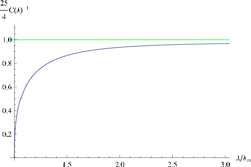
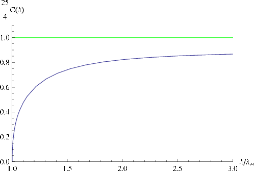 (a)
(b)
(a)
(b)
Independent of the precise value of , one can infer from the form of (B.25) that the parabola describing the repulson-free region for the self-dual and anti-self-dual 4-forms will touch at one, and only one, point, as is illustrated in 7, for generic values of .
There are several general lessons one can infer from the form of (B.25), the existence of one parameter family of deformation of space illustrated in figure 6, the general layout of the parabolas as is illustrated in figure 7, and the numerical values of as is illustrated in figure 11. These lessons can be summarized as follows
- •
Unlike in the case of the , the position of the parabola will depend on the values of because is non-vanishing in general.
- •
In the limit where asymptotes to , the red parabolas will degenerate and disappear from the phase diagram since is diverging there.
- •
Also, in the limit, the position of the parabola is independent of since is going to zero there.
The region inside the green parabola in the limit appears to be special, where the geometry asymptotes in the IR to the warped squashed cone of [51], except that the D2 charge are such that the geometry is skew-whiffed. In other words, although the IR of the theory appears to be breaking supersymmetry, it appears nonetheless to be conformal.

The broad picture is that for every choice of , , , , and , there is specific dynamical system for which we have partial understanding of the dynamics through the dual supergravity description. , , , and are discrete parameters. Continuous parameters and are constrained once all the discrete parameters are fixed. Alternatively for fixed , , and , which constrains , one can illustrate the phase diagram as a function of and as is illustrated in figure 7. As we noted in number of contexts, the points along the boundary of the parabolic region are special from the gravity point of view, in that the 2-brane source at the core is identically zero. Remarkably, it turns out that one can chose a unique value of for (almost) every choice of , , , and so that we sit at this special point on the boundary of the parabolic region as is illustrated in figure 12. The regions illustrated in light red and light green corresponds to various slices of the boundary of the red and green parabolas of figure 7. This foliation turns out not to cover the entire range of of because as approach , the green parabola for the repulson-free region of the do not collapse to zero size. However, a natural extension of as a function of , , , and is to set it equal to the constant value . In this way, as a function of these variables will be continuous, giving rise to a smoothly connected family of supergravity solutions. The supergravity solution itself will also be singularity free, except at the boundary of the parabola where there will be a conical singularity, whose base is the squashed , in the core region.
For all of the points parameterized by , , , , and in the phase diagram illusterated in figure 7, the geometry in UV asymptotes to that of which preserves supersymmetry. For all points outside the red parabolas, however, this supersymmetry is broken. Since in the perspective of the field theory dual, this is dynamical breaking of supersymmetry, one expects to find the corresponding Goldstone fermions. At least in the region inside the green parabola of figure 7, a gravity description of these theories in the broken supersymmetry phase is availble. For these geometires, one can show that there are precisely two normalizable fermion zero modes, following the analysis of [57].
In [20], a “tri-axial” family of holonomy manifold was constructed, further broading the arsenal of known holonomy manifolds. These authors then identified a one parameter subset of this family, which they named . We expect much of what we found for the to carry over to the case as well.
References
- [1] J. M. Maldacena, “The large limit of superconformal field theories and supergravity,” Adv. Theor. Math. Phys. 2 (1998) 231–252, hep-th/9711200.
- [2] N. Itzhaki, J. M. Maldacena, J. Sonnenschein, and S. Yankielowicz, “Supergravity and the large limit of theories with sixteen supercharges,” Phys. Rev. D58 (1998) 046004, hep-th/9802042.
- [3] J. Bagger and N. Lambert, “Gauge symmetry and supersymmetry of multiple M2-branes,” Phys. Rev. D77 (2008) 065008, arXiv:0711.0955.
- [4] A. Gustavsson, “Algebraic structures on parallel M2-branes,” arXiv:0709.1260.
- [5] J. H. Schwarz, “Superconformal Chern-Simons theories,” JHEP 11 (2004) 078, hep-th/0411077.
- [6] M. Van Raamsdonk, “Comments on the Bagger-Lambert theory and multiple M2- branes,” JHEP 05 (2008) 105, arXiv:0803.3803.
- [7] O. Aharony, O. Bergman, D. L. Jafferis, and J. Maldacena, “ superconformal Chern-Simons-matter theories, M2-branes and their gravity duals,” JHEP 10 (2008) 091, arXiv:0806.1218.
- [8] T. Kitao, K. Ohta, and N. Ohta, “Three-dimensional gauge dynamics from brane configurations with -fivebrane,” Nucl. Phys. B539 (1999) 79–106, hep-th/9808111.
- [9] O. Bergman, A. Hanany, A. Karch, and B. Kol, “Branes and supersymmetry breaking in 3D gauge theories,” JHEP 10 (1999) 036, hep-th/9908075.
- [10] A. Hashimoto and P. Ouyang, “Supergravity dual of Chern-Simons Yang-Mills theory with superconformal IR fixed point,” JHEP 10 (2008) 057, arXiv:0807.1500.
- [11] O. Aharony, O. Bergman, and D. L. Jafferis, “Fractional M2-branes,” JHEP 11 (2008) 043, arXiv:0807.4924.
- [12] O. Aharony, A. Hashimoto, S. Hirano, and P. Ouyang, “D-brane Charges in Gravitational Duals of 2+1 Dimensional Gauge Theories and Duality Cascades,” JHEP 01 (2010) 072, arXiv:0906.2390.
- [13] I. R. Klebanov and M. J. Strassler, “Supergravity and a confining gauge theory: Duality cascades and SB-resolution of naked singularities,” JHEP 08 (2000) 052, hep-th/0007191.
- [14] E. Witten, “Supersymmetric index of three-dimensional gauge theory,” hep-th/9903005.
- [15] J. M. Maldacena and H. S. Nastase, “The supergravity dual of a theory with dynamical supersymmetry breaking,” JHEP 09 (2001) 024, hep-th/0105049.
- [16] K.-M. Lee, E. J. Weinberg, and P. Yi, “The moduli space of many BPS monopoles for arbitrary gauge groups,” Phys. Rev. D54 (1996) 1633–1643, hep-th/9602167.
- [17] A. Sen, “Dyon - monopole bound states, selfdual harmonic forms on the multi - monopole moduli space, and SL(2,Z) invariance in string theory,” Phys. Lett. B329 (1994) 217–221, hep-th/9402032.
- [18] M. Cvetic, G. W. Gibbons, H. Lu, and C. N. Pope, “New complete non-compact manifolds,” Nucl. Phys. B620 (2002) 29–54, hep-th/0103155.
- [19] S. Gukov and J. Sparks, “M-theory on manifolds. I,” Nucl. Phys. B625 (2002) 3–69, hep-th/0109025.
- [20] M. Cvetic, G. W. Gibbons, H. Lu, and C. N. Pope, “Cohomogeneity one manifolds of and holonomy,” Phys. Rev. D65 (2002) 106004, hep-th/0108245.
- [21] S. Gukov and D. Tong, “D-brane probes of special holonomy manifolds, and dynamics of three-dimensional gauge theories,” JHEP 04 (2002) 050, hep-th/0202126.
- [22] E. Witten, “Solutions of four-dimensional field theories via M-theory,” Nucl. Phys. B500 (1997) 3–42, hep-th/9703166.
- [23] A. Hanany and E. Witten, “Type IIB superstrings, BPS monopoles, and three- dimensional gauge dynamics,” Nucl. Phys. B492 (1997) 152–190, hep-th/9611230.
- [24] K. Dasgupta and S. Mukhi, “Brane constructions, fractional branes and anti-de Sitter domain walls,” JHEP 07 (1999) 008, hep-th/9904131.
- [25] A. Giveon and D. Kutasov, “Seiberg Duality in Chern-Simons Theory,” Nucl. Phys. B812 (2009) 1–11, arXiv:0808.0360.
- [26] A. Giveon and D. Kutasov, “Gauge symmetry and supersymmetry breaking from intersecting branes,” Nucl. Phys. B778 (2007) 129–158, hep-th/0703135.
- [27] C. Bachas and M. B. Green, “A classical manifestation of the Pauli exclusion principle,” JHEP 01 (1998) 015, hep-th/9712187.
- [28] C. P. Bachas, M. B. Green, and A. Schwimmer, “(8,0) quantum mechanics and symmetry enhancement in type I’ superstrings,” JHEP 01 (1998) 006, hep-th/9712086.
- [29] J. P. Gauntlett, G. W. Gibbons, G. Papadopoulos, and P. K. Townsend, “Hyper-Kähler manifolds and multiply intersecting branes,” Nucl. Phys. B500 (1997) 133–162, hep-th/9702202.
- [30] S. A. Cherkis and A. Hashimoto, “Supergravity solution of intersecting branes and AdS/CFT with flavor,” JHEP 11 (2002) 036, hep-th/0210105.
- [31] D. Tong, “NS5-branes, T-duality and worldsheet instantons,” JHEP 07 (2002) 013, hep-th/0204186.
- [32] D. Marolf, “Chern-Simons terms and the three notions of charge,” hep-th/0006117.
- [33] D. S. Freed and E. Witten, “Anomalies in string theory with D-branes,” hep-th/9907189.
- [34] G. W. Gibbons, “The Sen conjecture for fundamental monopoles of distinct type,” Phys. Lett. B382 (1996) 53–59, hep-th/9603176.
- [35] H.-C. Kao and K.-M. Lee, “Selfdual Chern-Simons systems with an extended supersymmetry,” Phys. Rev. D46 (1992) 4691–4697, hep-th/9205115.
- [36] H.-C. Kao, “Selfdual Yang-Mills Chern-Simons Higgs systems with an extended supersymmetry,” Phys. Rev. D50 (1994) 2881–2892.
- [37] K. Becker and M. Becker, “Supersymmetry breaking, M-theory and fluxes,” JHEP 07 (2001) 038, hep-th/0107044.
- [38] O. Bergman and S. Hirano, “Anomalous radius shift in ,” arXiv:0902.1743.
- [39] C. V. Johnson, A. W. Peet, and J. Polchinski, “Gauge theory and the excision of repulson singularities,” Phys. Rev. D61 (2000) 086001, hep-th/9911161.
- [40] P. Brax, G. Mandal, and Y. Oz, “Supergravity description of non-BPS branes,” Phys. Rev. D63 (2001) 064008, hep-th/0005242.
- [41] O. DeWolfe, S. Kachru, and M. Mulligan, “A Gravity Dual of Metastable Dynamical Supersymmetry Breaking,” Phys. Rev. D77 (2008) 065011, arXiv:0801.1520.
- [42] I. Bena, M. Grana, and N. Halmagyi, “On the Existence of Meta-stable Vacua in Klebanov- Strassler,” arXiv:0912.3519.
- [43] O. Lunin, “Strings ending on branes from supergravity,” JHEP 09 (2007) 093, arXiv:0706.3396.
- [44] R. Bryant and S. Salamon, “On the construction of some complete metrices with expectional holonomy,” Duke Math. J. 58 (1989) 829.
- [45] G. W. Gibbons, D. N. Page, and C. N. Pope, “Einstein Metrics on , and Bundles,” Commun. Math. Phys. 127 (1990) 529.
- [46] A. Loewy and Y. Oz, “Branes in special holonomy backgrounds,” Phys. Lett. B537 (2002) 147–154, hep-th/0203092.
- [47] P. Bizon, T. Chmaj, G. W. Gibbons, and C. N. Pope, “Gravitational solitons and the squashed seven-sphere,” Class. Quant. Grav. 24 (2007) 4751–4776, hep-th/0701190.
- [48] G. C. Giecold, “Finite-Temperature Fractional D2-Branes and the Deconfinement Transition in 2+1 Dimensions,” JHEP 03 (2010) 109, arxiv:0912.1558.
- [49] M. J. Duff, B. E. W. Nilsson, and C. N. Pope, “Spontaneous supersymmetry breaking by the squashed seven sphere,” Phys. Rev. Lett. 50 (1983) 2043.
- [50] M. J. Duff, B. E. W. Nilsson, and C. N. Pope, “Kaluza-Klein Supergravity,” Phys. Rept. 130 (1986) 1–142.
- [51] H. Ooguri and C.-S. Park, “Superconformal Chern-Simons Theories and the Squashed Seven Sphere,” JHEP 11 (2008) 082, arXiv:0808.0500.
- [52] D. Martelli and J. Sparks, “ duals from M2-branes at hypersurface singularities and their deformations,” JHEP 12 (2009) 017, arXiv:0909.2036.
- [53] E. Witten, “On flux quantization in M-theory and the effective action,” J. Geom. Phys. 22 (1997) 1–13, hep-th/9609122.
- [54] L. Alvarez-Gaume and E. Witten, “Gravitational Anomalies,” Nucl. Phys. B234 (1984) 269.
- [55] A. J. Niemi and G. W. Semenoff, “Axial Anomaly Induced Fermion Fractionization and Effective Gauge Theory Actions in Odd Dimensional Space- Times,” Phys. Rev. Lett. 51 (1983) 2077.
- [56] A. N. Redlich, “Parity Violation and Gauge Noninvariance of the Effective Gauge Field Action in Three-Dimensions,” Phys. Rev. D29 (1984) 2366–2374.
- [57] M. J. Duff, H. Lu, C. N. Pope, and E. Sezgin, “Supermembranes with fewer supersymmetries,” Phys. Lett. B371 (1996) 206–214, hep-th/9511162.
- [58] M. Berkooz and S.-J. Rey, “Non-supersymmetric stable vacua of M-theory,” JHEP 01 (1999) 014, hep-th/9807200.
- [59] M. Berkooz and A. Kapustin, “A comment on nonsupersymmetric fixed points and duality at large N,” Adv. Theor. Math. Phys. 3 (1999) 479–494, hep-th/9903195.
- [60] I. R. Klebanov and A. A. Tseytlin, “Gravity Duals of Supersymmetric Gauge Theories,” Nucl. Phys. B578 (2000) 123–138, hep-th/0002159.
- [61] P. Ouyang, “Holomorphic D7-branes and flavored gauge theories,” Nucl. Phys. B699 (2004) 207–225, hep-th/0311084.
- [62] F. Benini, F. Canoura, S. Cremonesi, C. Nunez, and A. V. Ramallo, “Backreacting Flavors in the Klebanov-Strassler Background,” JHEP 09 (2007) 109, arXiv:0706.1238.
- [63] I. R. Klebanov and E. Witten, “Superconformal field theory on threebranes at a Calabi-Yau singularity,” Nucl. Phys. B536 (1998) 199–218, hep-th/9807080.
- [64] S. Mukhi, N. V. Suryanarayana, and D. Tong, “Brane-antibrane constructions,” JHEP 03 (2000) 015, hep-th/0001066.
- [65] A. Giveon and D. Kutasov, “Brane dynamics and gauge theory,” Rev. Mod. Phys. 71 (1999) 983–1084, hep-th/9802067.
- [66] S. Mukhi and N. V. Suryanarayana, “A stable non-BPS configuration from intersecting branes and antibranes,” JHEP 06 (2000) 001, hep-th/0003219.
- [67] K. Behrndt, “About a class of exact string backgrounds,” Nucl. Phys. B455 (1995) 188–210, hep-th/9506106.
- [68] R. Kallosh and A. D. Linde, “Exact supersymmetric massive and massless white holes,” Phys. Rev. D52 (1995) 7137–7145, hep-th/9507022.
- [69] M. Cvetic and D. Youm, “Singular BPS saturated states and enhanced symmetries of four-dimensional supersymmetric string vacua,” Phys. Lett. B359 (1995) 87–92, hep-th/9507160.
- [70] work in progress.
- [71] A. H. Chamseddine and M. S. Volkov, “Non-Abelian vacua in , gauged supergravity,” JHEP 04 (2001) 023, hep-th/0101202.
- [72] L. Hostler and R. H. Pratt, “Coulomb Green’s Function in Closed Form,” Phys. Rev. Lett. 10 (1963) 469–470.
- [73] M. Abramowitz and I. A. Stegun, Handbook of Mathematical Functions with Formulas, Graphs, and Mathematical Tables. Dover, New York, 1964.