On building minimal automaton for subset matching queries
Abstract
We address the problem of building an index for a set of strings, where each string location is a subset of some finite integer alphabet of size , so that we can answer efficiently if a given simple query string (where each string location is a single symbol) occurs in the set. That is, we need to efficiently find a string such that for every . We show how to build such index in average time, where is the average size of the subsets. Our methods have applications e.g. in computational biology (haplotype inference) and music information retrieval.
Keywords: algorithms; approximate string matching; subset matching; finite-state automaton minimization
1 Introduction
Let be an ordered integer alphabet. We are given a set of strings, called a dictionary. Each location of the string is a subset of , i.e. for every and . A string is called simple if its each location is a single symbol from , i.e. . The simple query string matches the dictionary string iff for and . We consider the following two problems:
Problem 1
Decide if matches any string in .
Problem 2
Retrieve the set such that matches for all .
In particular, we set out to efficiently build a small index for such that both problems can be solved in time.
Efficient solution of these problems have applications in computational biology, in matching DNA () or protein () strings, or in haplotype inference () [9, 10]. Finally, note that if is either or for all , then we have a special case called wild-card matching [3]. Another special case is -matching (see e.g. [2]), where we have where , and . These variants have applications in indexing natural language words and in music information retrieval.
1.1 Related work
Assume that the longest string in has length and that for every there are at most locations where . The immediate trivial solution to our problem would then be as follows. First generate all the simple strings of length that match a string in . Call the set of these strings . The size of is upper bounded by . The problem is now transformed to exact matching, so we can insert all strings in to some data structure that can answer whether a given simple query string matches a string in the data structure exactly. One such data structure is a path compressed trie [7] (cf. Sec. 2). This can be naïvely built in time and space. The queries can be answered in time.
This is also the approach in [10]. They give two non-trivial algorithms to construct the (path compressed) trie faster, namely in and time, yielding query times of and respectively (the latter method in fact uses two tries).
1.2 Our contributions
Inspired by [10], we also take the approach of computing the trie for as a starting point. However, instead of a trie, we directly build a pseudo-minimal (cf. Sec. 2.2) deterministic finite-state automaton (DFA) corresponding to the set ; i.e. our method does not explicitly generate the set . The resulting automaton can be used to solve Problems 1 and 2 in time. This automaton can be easily and efficiently minimized (again, cf. Sec. 2.2), so that the Problem 1 can still be solved in time. We also propose a form of path compression that can further save space and speed up the construction. We show that our construction works in . average time, where .
As shown experimentally, our algorithm can be orders of magnitude faster in construction time than the related naïve approach of first building a trie for , and then converting it to the minimal DFA, or directly building the minimal DFA from . The pseudo-minimal automaton is more efficient to construct than the true minimal automaton, and is in practice only slightly larger.
2 The algorithm
Let us define a DFA as , where is the set of states, is the initial state, is the set of accepting states and is the transition function. For convenience we also define for a string .
2.1 Prelude
Traditionally a trie [7] is described as being a rooted tree storing a set of (simple) strings. Each node has at most children, and the (directed) edges are labeled by the symbols in . In path compressed trie the unary paths are compacted to single edges, labeled by strings consisting of the concatenation of the symbols in the original path. In both cases, a path from the root to any node spells out a prefix of a subset of the strings stored in the trie, and that subset is stored in the subtree rooted at . The trie can be seen as a DFA in an obvious way; the root node corresponding to the state , and the labeled edges corresponding to .
We extend the DFA so that for the nodes we attach a list , storing the corresponding string identifiers. More formally, we define
| (1) |
where denotes the string spelled by the path from to , i.e. . Thus by generating all the strings that match a string in and building a DFA for , Problems 1 and 2 can be solved in time.
One of the problems of this approach is that can be large. A way to alleviate this is to minimize the DFA. There exists a large number of algorithms for this task [4]. Some of these can build the automaton incrementally, inserting one string at a time while maintaining the automaton in minimal state (e.g. [6]).
This can still be unnecessarily slow. Moreover, the result does not allow proper mapping between the states and the lists . E.g. if all the strings in are of equal length, the resulting minimal DFA would have only one accepting state. However, this automaton can still be used to solve Problem 1. Another solution is to construct a pseudo-minimal DFA [11, 5] still allowing mapping states or transitions to strings. We take a similar approach, although our definition of pseudo-minimal is somewhat different.
2.2 Pseudo-minimal DFA
We now present an algorithm that directly (i.e. our algorithm never deletes a state) constructs pseudo-minimal DFA from , without using a trie-like DFA as an intermediate step, or explicitly generating the set . Nevertheless, we first describe a particular (direct) way to build a trie-DFA, and then define a certain equivalence relation for the trie states, and show how we can during the construction avoid creating new states by identifying an equivalent state already present.
The algorithm can proceed recursively in either a depth-first or a breadth-first manner, with minor differences. We describe and give pseudo code for the breadth-first variant: the construction begins by inserting the starting state (root node) into queue of states; at each stage a state is dequeued and its children are computed and enqueued. The algorithm terminates when the queue becomes empty. As described above, each state will have an associated list , (, if ). We will denote the partially computed list as (). The following invariants are maintained: (a) when all the children (if any) of are enqueued, the state is fully computed and Eq. (1) is satisfied (post-condition); (b) when a state is enqueued, then the list satisfies Eq. (2) below (pre-condition):
| (2) |
I.e. iff matches a prefix of (note that , if the paths are not compressed). Thus the algorithm initializes
| (3) |
and enqueues . At each iteration, one state is dequeued, its “children” are initialized according to the pre-condition, and enqueued, and the post-condition for is computed. Given the list and , we define
| (4) |
If , then a transition is added, and enqueued. Note that is put into lists. The list is then computed as
| (5) |
That is, we keep only the strings that end in , and becomes an accepting state iff . All the lists and the list can be computed with a single pass over the the list . Alg. 1 gives the pseudo code.
This is repeated until the queue becomes empty. Note that this computes exactly the same trie as one would get by first generating and then inserting the strings one at a time. However, our bulk-insertion method is more easily improved.
We define the following relation between the states and :
| (6) |
which is clearly reflexive, symmetric, and transitive, i.e. an equivalence relation. The following is easy to notice:
| (7) |
where the language of is
| (8) |
Hence we will partition the states into equivalence classes, so that in the final DFA all states belong to a different class. Note that this does not result in a minimal DFA; i.e. we have that , while the implication would be required for a true minimal automaton. Note that by the definition we can still properly associate states with the lists and . So we can call the result pseudo-minimal DFA as in [11, 5], even when our definition should not be confused with the definition given in these papers
We need to maintain sets of pairs , where is a key that is used to insert and search the state , a representative of its equivalence class. The algorithm is now immediate: whenever we have computed a list , we search if it is present in a set ; if so, can be replaced by the corresponding node . In this case, is not enqueued, as an equivalent state is in the queue already. If is not present, we insert to , and enqueue . Alg. 2 gives the complete pseudo code, keeping the automaton in its pseudo-minimal state throughout the construction.
| 1 | |||
| 2 | for to do | ||
| 3 | for to do | ||
| 4 | |||
| 5 | if then | ||
| 6 | |||
| 7 | else | ||
| 8 | for do | ||
| 9 | return |
| 1 | ||||
| 2 | ||||
| 3 | ||||
| 4 | while not do | |||
| 5 | ||||
| 6 | ||||
| 7 | if then | |||
| 8 | for to do | |||
| 9 | if then continue | |||
| 10 | ||||
| 11 | if then | |||
| 12 | ||||
| 13 | ||||
| 14 | ||||
| 15 | ||||
| 16 | ||||
| 17 | return |
2.3 Using subsets for unary paths
For a moment consider a plain trie with a path compression. In this case the trie has nodes (states), independent of the pattern lengths (without path compression, this is multiplied by ). While this may save space in many cases, this is not always so. Consider e.g. the unrealistically pathological case, where contains only one string of length , namely . This means that all possible strings are present in , and no path compression can take place, as there simply are no unary paths (the minimal and pseudo-minimal DFAs would both have only states). We propose a slightly different, but much more effective, path compression.
Consider now a string in , and in particular that the string positions can be any subsets of (not necessarily just single symbols). Assume that , for some and . This means that there is no need to branch, since all the subsets are the same, and no symbol in can differentiate between any , . Hence we could add a transition from to (some) using the subset as a label. This does not pose any problems, as (when used in recognition) we can still test in time if . (Note that our pseudo-minimization algorithm effectively already handles this, i.e. under the above condition, for .)
More generally, given a node , and
| (9) |
then can be used as a string label in a compressed unary path.
The easiest way to utilize this is to use it only for unary paths to the leaves when . This is effectively achieved simply by replacing the line 15 in Alg. 2 by “if then Enqueue”. It would be relatively easy to use the path compression in any unary path, but as show in Sec. 3 this simple method can give huge savings in both time and space.
2.4 Analysis
Let us now consider the running time of Alg. 2, with (our) path compression on leaves. We assume that the subsets have average size , and that they are are randomly, uniformly and independently generated. At first we assume that there is a non-zero probability that two random subsets do not intersect (e.g. ).
The partition of can be implemented to take time. Each of the resulting new sets have average size , as for a random the probability that is . These sets are searched from , and possibly inserted (if not found). The size of is upper bounded by , the number of states in the resulting automaton. Hence insert/search can be implemented in worst case time with a number of radix-tree techniques, see e.g. [12, 1]. Therefore the total time per node is , i.e. , which is , assuming .
For a moment assume that we are building a plain trie, without path compression. Recall that by definition the length of the list is exactly . As described above, the length11 1 In the “worst case” there is only one “new” set, being exactly the same as its parent, ; but in this case the corresponding node would not branch, so the complexity would only improve. of each of the lists for the children of node is , so the lengths of the lists decrease exponentially when the depth of (i.e. ) increase, as . Hence when . The total number of states up to this depth is , that is, all the states have all the possible branches up to depth . As there are nodes at depth , the total length of all the lists at a depth is on average . Thus the total length of all the lists up to depth is .
Assume now (pessimistically) that path compression and pseudo-minimization take place only after depth . After this depth, the lists have length , (and will continue to shrink until ).There are only different lists of length , but at the same time there are states (with associated lists), so by the pigeonhole principle many of the states must be equivalent, and are combined into a single state. However, due to path compression, the process terminates for any state having . Hence the number of states per level starts to decrease exponentially22 2 Note that without combining the equivalent states or the path compression, after depth the number of states would continue to increase exponentially, resulting in a full trie. after depth . That is, the total number of states is bounded by two geometric series, both having the largest term at depth , where the automaton is in its “widest”, i.e. the total number of states is asymptotically upper bounded by .
Summing up, the total time is on average
| (10) |
again assuming .
So far we have assumed that there is a non-zero probability that two random subsets do not intersect. Consider now the (rather uninteresting) case where the subset sizes are always (not just on average). At first, the process goes as before, the number of states increasing exponentially, and the list lengths decreasing exponentially. However, assume now, for simplicity, that for some state . Due to , the subsets and must intersect (where ). Thus the alphabet is effectively partitioned into four disjoint sets: ; ; ; . Group does generate any branches for . Symbols from , and generate branches, but these are combined (group-wise) by the minimization, resulting in at most one new state per group, call it . For (similarly for ), , and due to path compression, will have no descendants. The interesting case is . Note that cannot be empty, so , and hence the process repeats for . In other words, the process does not terminate until .
The situation is similar when . Note that after depth we have in any case, and because of the pseudo-minimization, there can be only different states with lists of length . Thus in general the “breadth” of the automaton will stay approximately the same after depth , and the total time is upper bounded by , where is the length of the strings in .
Finally, as the number of subsets of items is at most , the trivial upper bound for the worst case size of our data structure is . This should be contrasted with the bound of [10].
3 Experiments and final remarks
We have implemented the algorithms in C, and ran the experiments on 3.0GHz Intel Core2 with 2GB RAM, 4MB L2 cache, running GNU/Linux 2.6.23.
The implemented algorithms are: Pseudo-minimal DFA (PM DFA), as in Alg. 2; minimal DFA (M DFA); PM DFA with path compression (PM DFA PC) on leaves, as detailed in Sec. 2.3; plain trie; and trie with path compression on leaves (Trie PC), as in PM DFA PC. Some results for the Tries are not included, as they could not fit into the available RAM. M DFA was computed from PM DFA, as computing it from or the corresponding trie would have been totally intractable in most cases. We implemented the set in Alg. 2 with Patricia tries [12].
We have not implemented the methods in [10], but we show that the lower bound () for the size of their data structure can be several orders of magnitude larger than our empirical sizes. In fact, we can build reasonably small data structures for problem instances that are completely intractable with their methods.
Table 1 gives the results for some randomly generated instances. We used parameters , where is the length of the strings (all of equal length); denotes that in probability any string location contains a randomly selected subset of , where the size of the subset is randomly selected between ; otherwise (with probability ) the string location is a single random symbol from .
, Method time (s) PM DFA 0.828 476,365 M DFA 1.20 385,255 PM DFA PC 0.820 379,948 Trie 6.71 18,767,894 Trie PC 0.326 948,493 , PM DFA 1.42 680,906 M DFA 2.39 635,795 PM DFA PC 1.40 499,212 Trie PC 1.19 4,203,673 , PM DFA 6.50 1,335,251 M DFA 18.2 1,320,126 PM DFA PC 6.21 1,276,985 Trie PC 6.29 22,431,630 , PM DFA 6.28 1,331,241 M DFA 12.0 964,847 PM DFA PC 0.486 149,998 Trie 15.5 6,981,214 Trie PC 0.236 235,565 , PM DFA 0.954 118,474 M DFA 7.29 115,797 PM DFA PC 0.907 110,340
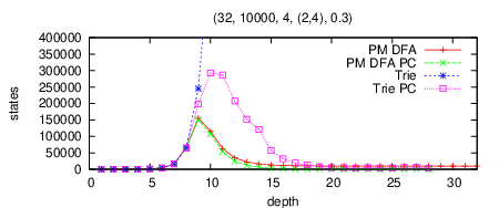
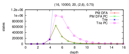
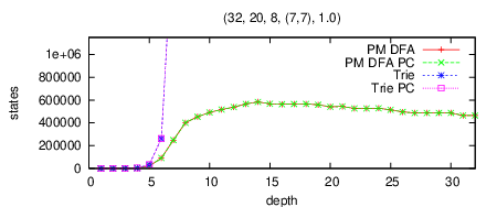
We report the number of states generated by the different methods, as well as the time in seconds, for some illustrative cases. As shown, the number of states generated is significantly smaller than in all cases, sometimes the difference being many orders of magnitude. PM DFA is usually only slightly larger than the true minimal DFA, while using path compression with PM DFA is usually smaller than M DFA. In some rare cases using path compression with a plain Trie is very competitive. Fig. 1 shows the exponential increase (depth ) and decrease (depth ) of the number of states as a function of the depth in the automaton / trie, and illustrates the behaviour when all subset sizes are .
Finally, we note that our methods have applications in on-line dictionary string matching, e.g. in -matching and -matching. It turns out that we can solve both problems in average time, which is optimal for -matching [8], for a dictionary of patterns of length , and a text of length . We leave the details for future work.
References
- [1] G. H. Badr and B. J. Oommen. Self-adjusting of ternary search tries using conditional rotations and randomized heuristics. Comput. J., 48(2):200–219, 2005.
- [2] E. Cambouropoulos, M. Crochemore, C. S. Iliopoulos, L. Mouchard, and Y. J. Pinzon. Algorithms for computing approximate repetitions in musical sequences. Int. J. Comput. Math., 79(11):1135–1148, 2002.
- [3] R. Cole, L. Gottliebd, and M. Lewenstein. Dictionary matching and indexing with errors and don’t cares. In Proceedings of STOC’04, pages 91–100, New York, NY, USA, 2004. ACM.
- [4] J. Daciuk. Comparison of construction algorithms for minimal, acyclic, deterministic, finite-state automata from sets of strings. In Proceedings of CIAA’02, LNCS 2608, pages 255–261. Springer, 2002.
- [5] J. Daciuk, D. Maurel, and A. Savary. Incremental and semi-incremental construction of pseudo-minimal automata. In Proceedings of CIAA’05, LNCS 3845, pages 341–342. Springer, 2005.
- [6] J. Daciuk, S. Mihov, B. W. Watson, and R. Watson. Incremental construction of minimal acyclic finite state automata. Computational Linguistics, 26(1):3–16, 2000.
- [7] E. Fredkin. Trie memory. Communications of the ACM, 3(9):490–499, 1960.
- [8] K. Fredriksson, V. Mäkinen, and G. Navarro. Flexible music retrieval in sublinear time. International Journal of Foundations of Computer Science (IJFCS), 17(6):1345–1364, 2006.
- [9] D. Gusfield. Haplotype inference by pure parsimony. In Proceedings of CPM’03, LNCS 2676, pages 144–155. Springer, 2003.
- [10] G. Landau, D. Tsur, and O. Weimann. Indexing a dictionary for subset matching queries. In Proceedings of SPIRE’07, volume 4726 of LNCS, pages 195–204. Springer, 2007.
- [11] D. Maurel. Pseudo-minimal transducer. Theoretical Computer Science, 231(1):129 – 139, 2000.
- [12] D. R. Morrison. Patricia—practical algorithm to retrieve information coded in alphanumeric. J. ACM, 15(4):514–534, 1968.