Linear acceleration emission in pulsar magnetospheresNote: Submitted to ApJ
Abstract
Linear acceleration emission occurs when a charged particle is accelerated parallel to its velocity. We evaluate the spectral and angular distribution of this radiation for several special cases, including constant acceleration (hyperbolic motion) of finite duration. Based on these results, we find the following general properties of the emission from an electron in a linear accelerator that can be characterized by an electric field acting over a distance : (i) the spectrum extends to a cut-off frequency , where is the Schwinger critical field and is the Compton wavelength of the electron. (ii) the total energy emitted by a particle traversing the accelerator is , in accordance with the standard Larmor formula, where is the fine-structure constant. (iii) the low frequency spectrum is flat for hyperbolic trajectories, but in general depends on the details of the accelerator. We also show that linear acceleration emission complements curvature radiation in the strongly magnetized pair formation regions in pulsar magnetospheres. It dominates when the length of the accelerator is less than the formation length of curvature photons, where is the radius of curvature of the magnetic field lines, and the Lorentz factor of the emitting particle. In standard static models of pair creating regions linear acceleration emission is negligible, but it is important in more realistic dynamical models in which the accelerating field fluctuates on a short length-scale.
Subject headings
plasmas — pulsars: general — radiation mechanisms: non-thermalI. Introduction
Linear acceleration emission is the radiation produced when a charged particle is accelerated in a direction parallel to its velocity. The resulting rectilinear trajectory is a special case. In astrophysics, it is expected to occur in the inner parts of a pulsar magnetosphere, where the strong magnetic field enforces one-dimensional motion on the electrons, and there is a non-zero electric field aligned with the magnetic field. The calculation of linear acceleration emission is complicated by the fact that relatively large sections of the trajectory radiate coherently (in a sense that will be made more precise in Section II). In the celebrated case of ‘hyperbolic’ motion, in which the acceleration measured in the instantaneous rest frame of the particle is constant, the entire trajectory remains coherent and it is impossible to define a local photon emission rate. Linear acceleration emission is a potentially important component of the electromagnetic cascades that occur in pulsars. These cascades are responsible for the materialization of the electrons and positrons that radiate in pulsar wind nebulæ, and, ultimately, make their way to Earth as a high-energy cosmic-ray component [23, e.g.,].
Early work on this problem in the context of pulsars treated the relativistic oscillator, in which the electric field is a linear function of position [33]. Linear solutions were considered by Melrose [18] and Kuijpers & Volwerk [14] who emphasized linear acceleration emission masers. Recently, the focus has shifted to superluminal, large-amplitude electrostatic waves. The particle trajectory and resulting emission in these waves was calculated using a semi-classical formalism by Rowe [24] and has been re-analyzed by Melrose et al. [20] and Melrose & Luo [19] who found and discussed some significant differences with Rowe’s results.
In this paper we compute the emissivity for linear acceleration in several special cases. The results enable us to estimate the emission in the general case, and we use this estimate to discuss the importance of the process in both static and dynamic models of the pair producing regions in pulsar magnetospheres, which we call “gaps”. Our method differs from that of Melrose et al. [20] and [19] in several respects. In particular, by avoiding the use of the ‘Airy integral approximation’ we resolve a puzzle they encountered concerning the applicability of Larmor’s formula to linear acceleration. We also drop the restriction to superluminally propagating disturbances, which enables us to treat static gaps, as well as those containing spatially isolated electric field structures such as double layers. Although the method and the details of the emissivity we find are substantially different, the main conclusions concerning the importance of linear acceleration emission in pulsars are consistent with those of Melrose & Luo [19]: it is unimportant for the parameters currently under discussion in static gap models of pulsars, but could be the dominant radiation mechanism in dynamic gap models.
The paper is organized as follows: in section II we briefly review the formalism of classical electrodynamics concerning the radiation of test particles in prescribed vacuum fields, emphasizing the role of the photon formation or coherence length. In section III we apply this formalism to the well-known problem of hyperbolic orbits (motion with constant acceleration in the particle’s rest frame) and derive a useful approximate representation of the angular and spectral distribution of radiated photons. In section IV we use the method of steepest descents to compute an approximate emissivity for a simple wave form that can describe a stationary or moving double layer. We also present an exact analytic solution for the spectrum emitted by a particle undergoing simple harmonic motion. In each case we demonstrate that the results agree with simple estimates based on the spectrum found for hyperbolic orbits. Finally, we discuss in section V the role of linear acceleration and curvature emission in pulsar gap models, comparing the relative importance of each process. Our conclusions are presented in section VI.
II. Emissivity
Consider a particle that moves in vacuum. The spectral and angular distribution of the energy it radiates is [27, e.g.,]
| (1) |
where is a unit vector in the direction of propagation of the emitted wave, and is the Fourier transform of the current:
| (2) | |||||
Here,
| (3) |
and are the position and velocity of the particle at time . The quantity can be identified as the phase of the emitted wave at the particle’s position, given that at . Thus,
| (4) | |||||
For sufficiently large , the exponential in (4) is sharply peaked around , which implies that the -integral can be written as a function of the particle velocity and its derivative at time , i.e., as the integral over the trajectory of a locally defined emissivity. For lower frequencies, however, this is not the case, and different parts of the trajectory contribute coherently to the emission. At any time , the section of the trajectory that contributes coherently is that over which the phases and do not differ by a large amount; i.e., one can identify the time over which changes by as a characteristic coherence time, or photon formation time [4, e.g].
For a relativistic particle whose trajectory has a radius of curvature , the coherence time is approximately , and a local emissivity can be defined, provided that the accelerating fields can be considered constant on this timescale. This is the normally encountered case of synchrotron radiation. However, for both ‘jitter’ radiation [31, 17, 13, e.g.,] and linear acceleration emission, the coherence time is not short compared to the timescale on which the accelerating fields vary.
For a particle that experiences acceleration only during a finite time interval, , the Fourier transform of the current can be written in terms of the trajectory within this interval:
| (5) |
as emphasized by Schwinger et al. [27]. Specializing to the case of linear acceleration emission in vacuum, and and the cosine of the angle between and is a constant. Therefore
| (6) | |||||
provided . The expressions (5) and (6) are the starting points of our analysis of the emissivity. It is worth noting that when (5) is inserted into (1) the emissivity can immediately be integrated over frequency and angle to give
| (7) | |||||
where , is the particle momentum -vector and the proper time. The integrand on the right-hand side of (7) is just the relativistic form of Larmor’s formula for the instantaneous power radiated. Thus, when integrated over a trajectory on which the acceleration is non-vanishing only within a finite time interval, this formula correctly gives the total radiated power. It is, nevertheless, incorrect to regard it as a truly instantaneous power, for example by associating a particular section of the trajectory with a part of the radiated power [e.g., 27, Chap. 37].
III. Hyperbolic motion
The trajectory of a particle moving with constant acceleration (as measured in its instantaneous rest frame) is called “hyperbolic” because of its shape in the -plane (the acceleration and velocity are assumed parallel). In classical electrodynamics in flat space, a hyperbolic trajectory results when a particle moves in a constant electric field which is parallel to its velocity, and also to the magnetic field, if any is present. The sometimes controversial literature on the problem of the radiation emitted by a particle on such a trajectory, goes back over a century — see, for example, Ginzburg [10]. In the last few decades, interest has arisen in the associated quantum effects, the Unruh Effect and Unruh Radiation [32, 6, 8, 29, e.g.,]. At least in the classical limit, the conceptual problems associated with hyperbolic motion disappear if the particle experiences acceleration during only a finite time-interval, outside of which it moves with constant velocity. We will assume this to be the case in the application to pulsars.
Consider a particle of charge and mass moving along the -axis in an electric field which is constant and of magnitude between and and vanishes elsewhere. Assuming the velocity is also directed along , the trajectory is
| (8) |
for . The length is the distance over which the electrostatic potential changes by :
| (9) | |||||
where is the Compton wavelength and is the electric field in units of the critical field — for an electron or positron this is the Schwinger field . The trajectory (8) is an exact solution of the classical equations of motion, including the Lorentz-Abraham-Dirac form of the radiation reaction force (which vanishes identically for ).
In a gap near a pulsar surface, the magnetic field is sufficiently strong that electrons and positrons rapidly decay into the Landau ground state. Then, if the radius of curvature of the field lines is large (see section V) the particle motion is approximately one-dimensional. The component along of the electric field induced by rotation of the star accelerates particles in a trajectory that can be approximated by (8), whereas the perpendicular component produces an -drift that can be transformed away. Static models of gaps assume the (parallel) field vanishes below the surface () and above a “pair-production front” at height , where photons produced in the gap create a sufficient number of charges to screen the field. Under pulsar conditions, one generally expects and (see Sect. V).
A particle that starts at rest at the surface and is accelerated upwards achieves a Lorentz factor at height . The energy radiated in passing from the surface to the pair production front can be computed from (5) or (6). For emission at , a simple approximation can be found by first transforming into the particle rest frame at proper time , when it has reached the position and a Lorentz factor . Denoting coordinates in this frame by , the trajectory is
| (10) | |||||
| (11) |
For photons of frequency emitted at , i.e., normal to in this frame, one finds [27]
| (12) |
where is a modified Bessel function of the second kind. This approximate solution involves extending the limits of the integration over the trajectory to , and is accurate provided the endpoints in the new (primed) frame of reference are far from the point at which the particle is at rest: . Returning to the frame in which the stellar surface is at rest, (12) describes the radiation emitted at . Therefore, exploiting the transformations , , where is the Doppler factor,
| (13) |
whence
| (14) |
where . The result can be checked by integrating over all frequencies, using the identity
| (15) |
to find
| (16) |
in agreement with the expression given by Schwinger et al. [27]. For small argument, , so that the low frequency spectrum is flat:
| (17) |
Using the asymptotic form of for large argument, one finds the high frequency spectrum:
| (18) |
which has a cut-off at the frequency
| (19) |
As expected, for relativistic particles, most of the energy is radiated close to the forward direction. The method applies only to radiation inside a small forwardly directed cone of opening angle , because otherwise is too close to the stellar surface. However, the region outside of this cone is not expected to contain significant power. The approximation also fails within a very small, forwardly directed cone, because the appropriate value of approaches or exceeds . This is potentially a more serious shortcoming, since it prevents one computing the emissivity on the beaming cone of a particle when it reaches its maximum Lorentz factor at the pair production front.
In fact, an explicit expression for the emission at can be written down by evaluating the integral over the orbit between the limits and :
| (20) | |||||
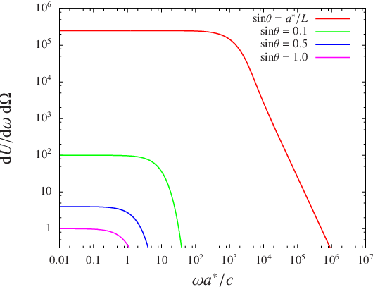
where is the modified Bessel function of the first kind and is the modified Struve function [3]. The spectrum at different angles, using this formula and equation (14) is shown in figure 1. At high frequencies one finds from (20) the asymptotic expression
| (21) |
In contrast with the emission at larger angle, this spectrum does not exhibit an exponential cut-off, but is a power law . This behavior is clearly related to the discontinuity in the electric field at . In reality, the pair production front is not a sharp boundary, but rather a region of finite width over which the field drops continuously to zero. The width of this region is determined by the distance over which the electric field can induce a substantial charge separation in the newly created pairs. Assuming these are born with Lorentz factor , where is the radius of curvature of the trajectory imposed by the strong magnetic field (see section V), the width of the front can be estimated to be roughly . Thus, the emission produced at small beaming angles is unlikely to differ qualitatively from emission at larger ones, and the entire pattern can be approximated as a hollow cone, with a cut-off frequency that increases towards the inner edge
Here, we have multiplied the spectrum (14) by normalization constant such that the total energy radiated matches that given by Larmor’s formula (7):
| (25) |
If the details of the emission on angular scales are unimportant, a “-function” approximation can be used. While the integration over solid angle cannot be found, a simple function that approximates the angular integrated spectrum is
| (26) |
The accuracy of this approximation can be seen in Figure 2 where the function is plotted together with the numerically integrated value of (III) for a range of .
The maximum photon energy produced can be reasonably approximated as
| (27) | |||||
As we discuss in section V, this implies that each electron that traverses the gap from to produces on average photons of frequency , where is the fine-structure constant.

IV. Spectra from motion in electrostatic waves
In this section we consider two special cases for which approximate or analytic expressions can be found. The first is an isolated structure containing a reversal of the the electric field. To facilitate the analysis, we choose a particle orbit of the form
| (28) |
with , i.e., the particle starts and finishes its orbit at rest, while its position suffers a displacement of . The maximum particle speed is . The electric field at the position of the particle is
| (29) |
Of the many functions that can provide such a trajectory, those representing an isolated structure that is either static or moving at constant, subluminal velocity (which is nowhere equal to the particle speed) are perhaps the simplest that are physically realistic. In the static case, the electric field is simply
where , but must be constructed using a simple algorithm in the moving case. Examples of these structures are shown in Fig. 3. If they accelerate particles to relativistic velocity, i.e., , they have the property that the maxima of the electric field are separated in space by roughly and have magnitude . Note that these are not self-consistent structures; they have been chosen to illustrate the properties of linear acceleration radiation.

From (6), allowing the limits , one finds
| (33) | |||||
| (34) |
This integral can be approximated using the method of steepest descents. As a function of complex argument , has a suitable saddle-point at , (). The result is best expressed in terms of the angle between the direction of propagation of the photon and the -axis, as measured in a frame moving along this axis at speed , in which case
| (35) |
and one arrives at the expression:
| (36) |
Thus, the spectrum rises linearly with frequency up to a cut-off at
| (37) |
Apart from the low frequency spectrum, which in any case is not reliably given by the method of steepest descents, this spectrum is roughly the same as that emitted by a particle experiencing uniform acceleration in a field over a distance , given in (27).
The second case we consider is motion in a periodic wave. To find an analytic solution, we choose a particularly simple particle orbit
| (38) |
I.e., the particle undergoes simple harmonic motion in one dimension. The spectrum produced by a particle with such a trajectory has previously been calculated by Schott [26]. The electric field at the position of the particle in this case is
| (39) |
which, as in the previous case, has maxima of the electric field separated in space by with magnitude . Thus, if the particle becomes highly relativistic, the field is large, but is confined to a small spatial region. Since the motion of the particle is periodic, the spectrum consists of harmonics of the oscillation frequency . The resulting power, averaged over one oscillation period, is
| (40) |
where
| (41) |
which clearly demonstrates the discrete nature of the spectrum. An alternative derivation to that of Schott [26] is given in the appendix. Equation (41) represents the average power radiated, in the -th harmonic, into a unit solid angle at an angle to the oscillation axis. For (see below) the power radiated in each harmonic at a fixed angle is proportional to . Fig. 4 shows a plot of this function for different emission angles.
When is large, the distance between neighboring harmonics becomes comparatively small, and the spectrum can be considered effectively as a continuum. The transformation to a continuous frequency spectrum can be made by formally replacing the summation in equation (40) by an integral
Taking the asymptotic value of the resulting expression, we find, in terms of the angle measured in a frame moving at speed
| (42) |
where we have multiplied by a factor to give the average energy emitted in each period, The critical frequency in this case is
| (43) |
This result is very similar to the approximate expression for an isolated structure, provided the strength of the electric field and its spatial extent coincide.

Approximate expressions for the emission produced by a relativistic oscillator have been found by Wagoner [33] and Melrose & Luo [19]. These share several properties with the simpler cases presented here. To compare with the emission from a hyperbolic trajectory, note that the electric field varies only linearly over the wave period, so that its effective spatial extent is . The effective field strength, on the other hand is . According to (27) a cut-off is expected at , as found by the above authors. The low frequency spectrum, however, is more sensitive to the wave form, with the oscillator having , whereas the low frequency spectrum radiated by the hyperbolic orbit is flat.
V. Application to pulsars
Pulsars are thought to lose their rotational energy in a relativistic wind that contains a large number of electron-positron pairs [12, for a review, see]. These pairs presumably materialize in an electromagnetic cascade initiated by electrons that are accelerated in the strong inductive electric fields surrounding the star. Recent observations indicate that gamma-ray pulses are unlikely to be produced close to the star [2, 1]. However, this is not necessarily the region where the pairs materialize, the location of which is still unknown. Detailed models of the electromagnetic cascades have been constructed [11, 7, reviewed in], but these face difficulties in accounting for the observations [1, 9, 30].
The radiation processes thought to be important in pulsar gap models are curvature radiation and inverse Compton scattering (both resonant and non-resonant). Linear acceleration emission is closely related to curvature radiation, since they both depend on the configuration of the large-scale electromagnetic fields anchored in the star. Inverse Compton scattering, on the other hand, depends not only on the local magnetic field strength, but also on the target photon population. Consequently, to assess the possible role of linear acceleration emission, we compare its spectrum and luminosity to the standard expressions describing curvature radiation.
The acceleration region or “gap” can be characterized by its height , and the potential drop across it. Assuming the electric field to be uniform, it can be expressed in units of the Schwinger field as
| (44) |
Denoting by the radius of curvature of the magnetic field lines in the gap, the characteristic or cut-off frequencies of linear acceleration emission, , and curvature emission, , are
| (45) | |||||
| (46) |
The energy radiated as linear acceleration emission, and as curvature radiation by a single electron that traverses the gap is
| (47) | |||||
| (48) |
These expressions show that linear acceleration emission and curvature radiation are complementary rather than competing processes. Each of them is an approximate evaluation of the radiation emitted by a charge accelerated along a curved trajectory, computed according to classical electrodynamics. In the case of linear acceleration emission, the approximation of large radius of curvature is used. In the case of curvature emission, the particle’s acceleration parallel to its velocity is neglected. If the system is such that , i.e., if the formation length for curvature photons is smaller than the acceleration region, then the radiation is well described by a local emissivity, and this can be evaluated from the standard curvature formulas, because the change in Lorentz factor is small within the photon formation length. On the other hand, if , the photon formation length is roughly equal to the size of the system and it is impossible to define a local emissivity. In this case, it is inconsistent to use the expressions derived for curvature radiation, since they apply only when the formation length is limited by the curvature of the trajectory. When the formation length is instead limited by the size of the acceleration region, the expressions derived for linear acceleration emission are applicable.
Note that these arguments do not apply to particles that are accelerated externally and are injected into the gap with . In this case, the effects of the longitudinal electric field are small and can be treated using a linear theory [18]. Strictly speaking, the arguments also do not apply if the particle is accelerated after leaving the gap — for example, if it continues to propagate along a curved field line without linear acceleration. However, in this case the local emissivity for curvature radiation can be used to describe the additional radiation.
Note that the average number of photons emitted by a particle as it traverses a photon formation length is . This is true both for linear acceleration emission and curvature (and synchrotron) radiation. For a classical picture to be valid, the energy of the radiated photon must be small compared to the energy of the radiating particle. In the case of linear acceleration emission this implies . Therefore, since the energy radiated is , classical linear acceleration emission cannot lead to a saturation of the acceleration process, in the sense of limiting . This is consistent with the fact that the radiation reaction force vanishes at all points on the trajectory except the end points. Classical curvature radiation, on the other hand, does saturate the acceleration, if the region exceeds a size given by
| (49) |
Gaps in pulsar magnetospheres can be divided into two types: vacuum gaps [28, 25] and gaps produced by space-charge limited flow [5]. The electric field is produced by the rotation of the strong surface magnetic field with G. In vacuum gaps, it may be as high as times the rotation speed/, and it is convenient to express it in terms of this value by introducing the parameter according to
| (50) | |||||
where , is the ratio of the stellar radius to the light-cylinder radius , is the pulsar period measured in seconds, and we have used the standard estimate for the surface magnetic field from the rate of loss of rotational energy
| (51) |
where is the rate of change of pulsar period times .
The presence of space-charge limits the electric field to much smaller values. When the effects of frame-dragging are taken into account [22, 21] one finds
| (52) | |||||
where, in analogy with (50), we have introduced the parameter .
The ratio of the system size to the formation length for curvature photons determines which radiation mechanism is appropriate in a particular gap. This condition can be formulated in terms of a critical Lorentz factor:
where we have written the radius of curvature of the field lines in units of the light cylinder radius, , and have inserted the expressions (50) and (52) for the accelerating fields. If (), curvature radiation (linear acceleration emission) is the appropriate description. Alternatively, the curvature photon formation length can be evaluated:
According to (V), curvature radiation is an appropriate description of the radiation from a vacuum gap (space-charge flow limited gap) provided its height exceeds roughly (). Note, however, that these conditions are relaxed (in the sense that the critical gap size is reduced) if the radius of curvature of the field lines is small compared to the light-cylinder radius, and also if the accelerating field fails to reach the full value given by (50) or (52) — both of which were assumed in the original Ruderman & Sutherland [25] model.
In current static models, the assumed gap heights greatly exceed , so that linear acceleration emission does not play a role. Recently, however, time-dependent gap models have been proposed [15, 30]. These models assume accelerating fields that are of the order of, or larger than the vacuum field given in (50). In addition, time-dependent screening leads to structure on a length scale determined essentially by the electron inertial length , where is the local plasma frequency. Estimating the electron/positron charge density as roughly equal to the charge-density required to screen the electric field (the “Goldreich-Julian” density) implies
| (59) |
so that
Therefore, linear acceleration emission is an essential ingredient in these models, because the formation length for curvature radiation photons substantially exceeds the anticipated length-scale of the structure in the accelerating electric field.
VI. Conclusions
The radiation produced by a particle whose acceleration is parallel to its velocity, linear acceleration emission, has been investigated for a number of special cases. Particle motion of this type is expected to occur in the intense magnetic fields close to the surface of a pulsar. The emission produced by these particles is conceptually difficult due to the macroscopic size of the photon formation length. For the particular case of hyperbolic motion, corresponding to acceleration in a uniform electric field, the formation length is comparable to the length of the entire accelerating region. Linear acceleration emission is similar to both synchrotron and curvature radiation in the sense that a photon is emitted with a probability when a particle traverses a formation length. The essential properties of the radiation produced by a particle on a hyperbolic trajectory can be understood in terms of two key parameters: the length of the hyperbolic part of the trajectory, and the length over which the particle increases its energy by . Some generic features of the emission mechanism in different electric field configurations can also be described using these quantities. In particular, provided and are interpreted appropriately (see section IV for some examples) the critical frequency can be expressed as .
Current models of pair production in pulsar magnetospheres typically assume that high energy photons that induce the secondary pair cascade, are produced via either curvature radiation or inverse-Compton scattering. An alternative to these processes is linear acceleration emission, as investigated by Melrose & Luo [19]. We have demonstrated that this process is in fact complementary to curvature radiation, the transition between the two regimes depending only on the ratio of the system size to the formation length of curvature photons. For existing static polar gap models, linear acceleration is unlikely to play an important role, although this relies on the environmental parameters being close to the canonical values. The limits for both vacuum gap models and space-charge limited models are presented in section V.
Recent numerical studies provide evidence that the above stationary models are unstable to perturbations [15, 30, e.g.]. Several analytic models have been developed in which particles are accelerated in large amplitude electrostatic waves that propagate parallel to the magnetic field [see e.g. 16, and references therein]. Since the characteristic length scale of the electric fields in these models is on the order of the electron inertial length, linear acceleration emission is likely to be a more appropriate description of the resulting radiation.
| (63) |
where . Using Poisson’s sum formula
| (64) |
and noting that is positive, we find
| (65) |
The integral in this equation can be expressed in terms the Bessel functions
| (66) |
where we have exploited the integral form of the Bessel function
| (67) |
Finally using the identity
| (68) |
the power radiated in the -th harmonic is
| (69) |
with
| (70) |
The validity of this result can be checked by comparing against Larmor’s formula Eq. (7). This can be done straightforwardly using the identity
| (71) |
and subsequently integrating over solid angle. Multiplying the resulting answer by the period of the waves gives the total energy radiated per oscillation
| (72) |
It is easily verified that this agrees exactly with Eq. (7).
The asymptotic expression for Bessel functions of large order and argument is [e.g 34, p. 249]
| (73) |
with . Thus, using the asymptotic expression for the modified Bessel functions with large argument, the spectrum at high harmonics is
| (74) |
References
- [1] Abdo, A. A. et al. 2009, Science, 325, 848
- [2] Abdo, A. A., & the Fermi LAT collaboration. 2009, ArXiv e-prints, 0910.1608
- [3] Abramowitz, M., & Stegun, I. A. 1972, Handbook of Mathematical Functions (New York: Dover)
- [4] Akhiezer, A. I., & Shul’ga, N. F. 1987, Soviet Physics Uspekhi, 30, 197
- [5] Arons, J., & Scharlemann, E. T. 1979, ApJ, 231, 854
- [6] Bell, J. S., & Leinaas, J. M. 1987, Nuclear Physics B, 284, 488
- [7] Cheng, K. S. 2009, in Astrophysics and Space Science Library, Vol. 357, Astrophysics and Space Science Library, ed. W. Becker, 481–+
- [8] Crispino, L. C. B., Higuchi, A., & Matsas, G. E. A. 2008, Reviews of Modern Physics, 80, 787
- [9] de Jager, O. C. 2007, ApJ, 658, 1177
- [10] Ginzburg, V. L. 1970, Soviet Physics Uspekhi, 12, 565
- [11] Harding, A. K. 2009, in Astrophysics and Space Science Library, Vol. 357, Astrophysics and Space Science Library, ed. W. Becker, 521–+
- [12] Kirk, J. G., Lyubarsky, Y., & Petri, J. 2009, in Astrophysics and Space Science Library, Vol. 357, Astrophysics and Space Science Library, ed. W. Becker, 421–+
- [13] Kirk, J. G., & Reville, B. 2010, ApJ, 710, L16
- [14] Kuijpers, J., & Volwerk, M. 1996, in Astronomical Society of the Pacific Conference Series, Vol. 105, IAU Colloq. 160: Pulsars: Problems and Progress, ed. S. Johnston, M. A. Walker, & M. Bailes, 181–+
- [15] Levinson, A., Melrose, D., Judge, A., & Luo, Q. 2005, ApJ, 631, 456
- [16] Luo, Q., & Melrose, D. 2008, MNRAS, 387, 1291
- [17] Medvedev, M. V. 2000, ApJ, 540, 704
- [18] Melrose, D. B. 1978, ApJ, 225, 557
- [19] Melrose, D. B., & Luo, Q. 2009, ApJ, 698, 124
- [20] Melrose, D. B., Rafat, M. Z., & Luo, Q. 2009, ApJ, 698, 115
- [21] Muslimov, A., & Harding, A. K. 1997, ApJ, 485, 735
- [22] Muslimov, A. G., & Tsygan, A. I. 1992, MNRAS, 255, 61
- [23] Profumo, S. 2008, ArXiv e-prints, 0812.4457
- [24] Rowe, E. T. 1995, A&A, 296, 275
- [25] Ruderman, M. A., & Sutherland, P. G. 1975, ApJ, 196, 51
- [26] Schott, G. A. 1912, Electromagnetic Radiation (Cambridge: The University press)
- [27] Schwinger, J., DeRead, L. L., Milton, K. A., & Tsai, W.-y. 1998, Classical Electrodynamics (Perseus Books, Reading)
- [28] Sturrock, P. A. 1971, ApJ, 164, 529
- [29] Thirolf, P. G. et al. 2009, European Physical Journal D, 55, 379
- [30] Timokhin, A. N. 2009, ArXiv e-prints, 0912.5475
- [31] Toptygin, I. N., & Fleishman, G. D. 1987, Ap&SS, 132, 213
- [32] Unruh, W. G. 1976, Phys. Rev. D, 14, 870
- [33] Wagoner, R. V. 1969, ApJ, 158, 739
- [34] Watson, G. N. 1922, A treatise on the theory of Bessel functions (Cambridge: The University press)