Isolated Flat Bands and Spin-1 Conical Bands in Two-Dimensional Lattices
Abstract
Dispersionless bands, such as Landau levels, serve as a good starting point for obtaining interesting correlated states when interactions are added. With this motivation in mind, we study a variety of dispersionless (“flat”) band structures that arise in tight-binding Hamiltonians defined on hexagonal and kagome lattices with staggered fluxes. The flat bands and their neighboring dispersing bands have several notable features: (a) flat bands can be isolated from other bands by breaking time-reversal symmetry, allowing for an extensive degeneracy when these bands are partially filled; (b) an isolated flat band corresponds to a critical point between regimes where the band is electron-like or hole-like, with an anomalous Hall conductance that changes sign across the transition; (c) when the gap between a flat band and two neighboring bands closes, the system is described by a single spin-1 conical-like spectrum, extending to higher angular momentum the spin-1/2 Dirac-like spectra in topological insulators and graphene; (d) some configurations of parameters admit two isolated parallel flat bands, raising the possibility of exotic “heavy excitons” and (e) we find that the Chern number of the flat bands, in all instances that we study here, is zero.
I Introduction
One of the reasons why dispersionless (or flat) bands are interesting is that they accommodate, when partially filled, an exponentially large number of states. This macroscopic degeneracy can be lifted when interactions are added, often leading to rich strongly correlated phenomena. The best known example is the fractional quantum Hall effect, which arises from the degeneracy within flat Landau bands for particles in a magnetic field.
In addition to the Landau problem, other models with flat bands have been studied at least since the 1970s, such as amorphous semiconductors [1, 2, 3]. This system is idealized by a lattice made up of clusters of sites. Both inter-cluster and intra-cluster hoppings are allowed. From a mathematical point of view, it turns out that the intra-cluster hopping term in the Hamiltonian is a projection operator, leading to the existence of flat bands [4, 5].
In the 1980s, flat bands were studied in relation to the Nielson-Ninomiya theorem [6] by Dagotto et al [7]. They showed that it is possible to escape the fermion-doubling problem at the price of having an extra flat band in the spectrum. In this way, the low energy degrees of freedom of the theory can be described as a single Weyl species.
More recently, Ohgushi et al [8] studied flux phases in the kagome lattice, which is the planar section of ferromagnetic textured pyrochlores. If the flux is staggered then electrons accumulate a spin Berry phase as they hop. This system contains isolated flat bands, i.e., they are protected by a gap. On the other hand, Bergman et al have studied flat bands without a gap in similar lattices [9] not threaded by fluxes. In their models, a flat band is degenerate with one or more other bands at a single point, and the touching is topologically protected. Each of the works above has identified interesting, but seemingly disconnected, properties of flat bands.
The purpose of this paper is to understand the different types of flat band spectra, the conditions to obtain them, and the properties that follow. This paper is organized around five main findings. First, flat bands can be isolated by breaking time-reversal symmetry (TRS). Second, isolated flat bands can be viewed as critical points. On either side of the phase boundary the flat band becomes positively or negatively curved, which corresponds to transitioning from a particle-like to a hole-like band. We also find an anomalous Hall effect on either side of the transition, whose sign depends on whether the band is electron-like or hole-like. Third, when the gap between a flat band and its neighboring bands closes with the flat band in the middle, the system is described by a single spin-1 conical-like spectrum. This extends to higher angular momentum the spin-1/2 Dirac-like spectra in topological insulators and in graphene. Fourth, one can obtain multiple (parallel) flat bands and we provide a concrete example of this case. Fifth, we find, for all examples studied here, that the Chern number of the flat bands is zero. So as opposed to Landau levels, we get no quantized Hall conductance for these particular flat bands.
(a)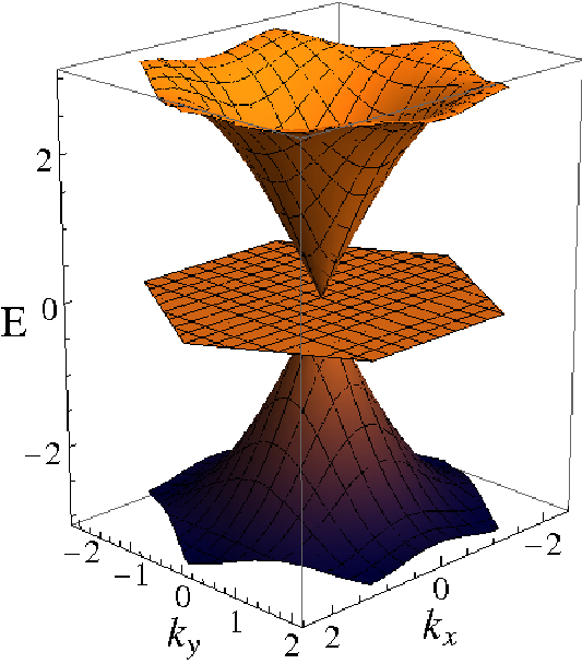 (b)
(b)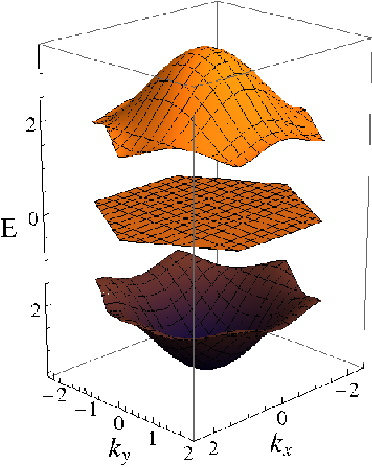
The model with which we will start our analysis is a simple kagome lattice with a tight-binding interaction and two staggered fluxes, and , on alternating triangles. Depending on the values of , dispersions can be classified into three types: (I) a flat band touches two linearly dispersing bands at the same point, where the linear bands are reminiscent of a “Dirac-like” point, but with spin-1 behavior, (II) an isolated flat band that is separated from bands above and below by a gap, and (III) a gapless flat band that touches a single massive energy band either above or below. The energy dispersions corresponding to types I and II are plotted in Fig. 1. Type III has been discussed recently [10, 11, 9] in hexagonal and kagome lattices without magnetic flux, and it was found that in this case the zero gap is protected by topological arguments [9]. Type III has been also shown to exhibit a topological insulator phase in the presence of spin-orbit interactions [12]. Type II appears when electrons accumulate a spin Berry phase as they hop from site to site, which is equivalent to both up and down triangles with the same magnetic flux [8]. Type I necessitates the staggered fluxes that we analyze below.
We will show that the condition for a flat band to occur at is . By changing the value of the fluxes in such a way that their sum differs slightly from , the flat band acquires a small curvature, which can be positive or negative depending on the values of . Interestingly, the band curvature implies that if the Fermi energy is chosen to be zero, then by tuning the fluxes it is possible to change the center of the band from an electron-like pocket to a hole-like pocket. This leads to an inversion of the sign of the anomalous Hall response [13]. Therefore, the flat band condition represents a quantum critical point separating two regions with different anomalous Hall responses.
Type I is remarkable in that it displays linearly dispersing modes, akin to those of graphene, but differing in two important ways. First, the conical points do not appear in pairs as in graphene, but instead there is only one such point within the first Brillouin zone (BZ) (see Fig. 1). Second, these are not Dirac fermions (this is why it is possible to evade the doubling problem), but instead the effective Hamiltonian in momentum space is of the form , where is the spin-1 angular momentum operator ( is the Fermi velocity). The spin-1-type spectrum (like the spin-1/2 Dirac-type spectrum of graphene) can be viewed as a single quantum spin in a magnetic field, as in Berry’s original work on quantum phases [14], but with the wave vector playing the role of the magnetic field. Type I does not require the breaking of TRS. However, we show that a gap can be opened while leaving the flat band untouched by breaking TRS, and thus type I is continuously connected to type II . In type II the degenerate states within the flat band are protected by the gap at finite temperature, and would provide a fertile base to construct correlated states.
Finally, we will generalize the above results on the kagome lattice to other lattices by a formulation similar to Straley [4], but again adding staggered fluxes. As an example, we take a hexagonal network, similar to graphene, but with three degrees of freedom at each site. We will consider two hopping strengths in this case, one for inter-site hopping between nearest neighbors () and one on each vertex for intra-site permutations between the three species (). Each permutation will be associated with a flux on the two sublattices of the honeycomb lattice. We will show that the kagome model can be obtained from this in the limit . Additionally, we will show that the honeycomb lattice admits two parallel flat bands that are isolated from each other and all other bands, which is a feature that the kagome lattice does not have.
II Flat zero-mode band in the staggered-flux kagome lattice
Consider the tight-binding Hamiltonian defined on a kagome lattice, where staggered fluxes and are applied within alternating triangles (“up” and “down” triangles, respectively), as shown in Fig. 2.

For convenience define the phase factors . Let , , and be the vectors pointing from the centers of an up triangle to its three down neighbors, and define , with . In momentum space, the Hamiltonian can be written as:
where is the hopping strength. The characteristic polynomial for this matrix is
| (5) |
where
and . The condition for a flat (-independent) band is obtained by setting the overall factor of in to zero,
| (6) |
which is equivalent to
| (7) |
Combining Eqs. (5)-(7) gives the following equation for the energy eigenvalues of the flat bands:
| (8) |
which has three possible solutions:
(a) flat band: this configuration is achieved for
,
(b) flat band: this configurations is achieved
for , with integer
valued numbers, and
(c) flat band: this configurations is achieved
for , with integer
valued numbers.
The cases (type III) are similar to those discussed in Refs. [10, 11, 9], where the flat band touches a parabolic electron-like band at its bottom (for ) or a hole-like band at its top (for ). Here, we shall focus instead in the case where the flat band is at . In Fig. 1 (types I and II) we show two particular choices for , which are representative of what we classify as types I and II spectra. Type I contains a cone vertex touching at the point , which we illustrate by setting and (this choice of phase can be interpreted as tight-binding hoppings for up triangles and for down triangles). Type II contains an isolated flat band, which we illustrate by setting (this choice can be interpreted as tight-binding matrix elements for hopping anti-clockwise or clock-wise around the triangles). Notice that because and one of the eigenvalues is , the other two eigenenergies must satisfy , so the spectrum is symmetric with respect to zero in both types I and II.
The general condition for nodal touching (type I) can be obtained by requiring that there is another eigenvalue, so that at least one other band touches the flat band. When such a solution exists, the derivative of the characteristic polynomial also has a zero at for some value of . This condition translates to
| (9) |
which admits three different solutions:
(A) Nodal point at :
this type I configuration is obtained if the condition
is satisfied, where is an integer,
and it is illustrated in Fig. 1 (type I),
(B) Nodal point at :
this type I configuration is obtained if the condition
is satisfied, where is an integer, and
(C) Nodal point at :
this type I configuration is obtained if the condition
is satisfied, where is an integer.
Even though types I and II are particle-hole symmetric with a flat band at and have staggered fluxes obeying the constraint , type II lacks the nodal conditions (A)-(C) mentioned above.
II.1 Nodal touching and the spin-1 cone
Let us now expand the Hamiltonian, in type I , near the vertex point for small . At the same time we move into type II by applying a slight flux offset from the condition for the touching: and . We will interpret as a “mass” term. To first order in and the Hamiltonian becomes:
| (10) | |||||
where . It is straightforward to check that the matrices
| (11a) | |||
| (11b) | |||
| (11c) |
satisfy the angular momenta algebra (along with the cyclic permutations of , , and ), and that they have eigenvalues , i.e., they form a spin-1 representation of SU().
The eigenvalues of the Hamiltonian (10) are , where is the eigenvalue of angular momentum along the direction . Therefore we obtain the three bands, with the flat band being the one with zero angular momentum. The other two bands describe the cone when , and two parabolic bands separated from the flat band by a gap when is non-zero. (A particular instance of the spectrum has recently also been predicted in optical lattices by Bercioux et al. [15])
The spin-1 structure has interesting topological properties, namely it can be viewed as a generalization of the Berry phase for the spin-1/2 spectrum of graphene. One implication is that, when the gap is open by breaking TRS, the upper and lower bands have a quantized Hall conductance. In the Appendix we explicitly compute the Chern number over the first Brillouin zone for the three bands.
II.2 Transitioning between electron and hole bands
We now consider deviations from the flat band condition for the case when the middle band is isolated, as in type II . For concreteness, consider the case . For small , the energy of the middle band will be close to , so we can obtain the dispersion for the middle band by dropping the cubic term in the characteristic polynomial ,
| (12) |
Expanding up to order and , one obtains
| (13) |
corresponding to a band mass for the middle band, so it has a hole-like dispersion for and an electron-like dispersion for , as depicted in Fig. 3. This trivial mathematical result is physically remarkable in that one can, in principle, change the character of a band from electron-like to hole-like by varying one parameter in the Hamiltonian.
(a)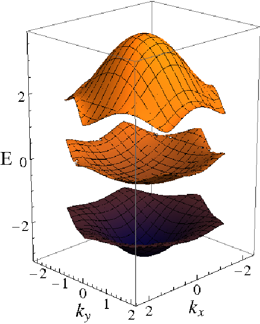 (b)
(b)
Notice that there is also a band shift , which adds to the chemical potential. There is an interesting result when the chemical potential is fixed to : the Fermi surface is pinned and independent of . It is best to see this effect prior to any perturbation in or expansion in . The Fermi surface is in this case the locus of points for which , those that satisfy . For the electron-like case, the Fermi sea is in the region bounded by the surface that contains the -point, whereas for the hole-like case the Fermi sea is the complementary region in the Brillouin zone. The anomalous Hall effect is given by the integral of the Berry curvature over the Fermi sea. As we show in the Appendix, the Chern number, the Berry curvature integrated over the complete Brillouin zone, for the middle flat band is zero. This means that the sum of the anomalous Hall effects for the electron-like and hole-like Fermi seas is zero. Thus, as one tunes across holding , the anomalous Hall effect will change sign. Of course, by tuning one can vary the anomalous Hall effect continuously.
II.3 Time-reversal and particle-hole symmetries
First, we discuss time-reversal symmetry. Consider a tight-binding model of spinless fermions described by
| (14) |
where is an annihilation fermionic operator and takes values on the first Brillouin zone. Under time-reversal transformation,
| (15) | |||||
For to be time-reversal invariant, one way would be to have . Looking at our Hamiltonian more carefully, though, we see that there is a freedom to redefine the hopping matrix elements without changing the fluxes and . This freedom can be mathematically described by the following gauge transformation:
| (16) |
where
| (17) |
Hamiltonians and related by the gauge transformation Eq. (16) represent physically equivalent descriptions of the system. The requirement of time-reversal symmetry, taking into account the gauge invariance given by Eq. (16), becomes then
| (18) |
from which we get the following conditions
| (19) |
Equation (19) immediately implies that symmetry under time reversal is satisfied if and , for integers and such that ( integer). This is exactly equivalent to the condition for such that the spectrum has a gapless flat band at , i.e., type I . Therefore, we conclude, for this given model, that in order to have an isolated flat band time-reversal symmetry must be broken.
Now consider particle-hole symmetry. The key observation is the following: when the spectrum of has three bands, as in the kagome lattice, particle-hole symmetry only exists when there is a flat band at and the two other bands have opposite energies. We have already worked out the conditions for the existence of a flat band in the kagome lattice to be , which also dictates the conditions for particle-hole symmetry (if the Hamiltonian is a traceless matrix). Notice that can be particle-hole symmetric without being time-reversal invariant. (A spin-1 cone is a situation where both symmetries are present.) We will use this important aspect later when we calculate the Chern number of the bands.
III Hexagonal Lattice Model
Having discussed the main properties of the kagome model, we now consider an alternative model defined on the hexagonal lattice. We will show that these models are closely related and that the kagome model is a limiting case of the hexagonal one. Even more interestingly the spectrum of the hexagonal model contains two parallel flat bands that are separated from each other and from all other bands by a gap.
III.1 Definition of the model
Consider a tight-binding model on a hexagonal lattice, where the particles have three flavors. Define the six-dimensional basis of particle operators ,, where is the flavor index, and are the two sublattices. In real space the Hamiltonian is:
| (20) | |||||
The first term (coupling ) is a nearest-neighbor hopping between the two sublattices that conserves the flavor index, but has correlated flavor-direction hopping controlled by ,
| (21) |
The second term (coupling ) is the on-site phase dynamics, where is the cyclical permutation matrix,
and the on-site flavor changing phase factors are (using the notation of Sec. II). In other words, inter-site hopping conserves the flavor index. Flavors can be permuted on-site, and each permutation is accompanied by an on-site phase factor . This Hamiltonian can be diagonalized analytically for particular values of .
III.2 Equivalence to the kagome model
Let us write the wave function basis as and work in momentum space. In this basis, our Hamiltonian takes the following six-dimensional form:
where
In the extreme case when , is block diagonal in the matrices and is trivial. It has two triply degenerate eigenvalues and eigenvectors . This corresponds to a “dimerized” state since the particles cannot hop between sublattices. (Recall that hoping between sublattices is directionally controlled by the flavor, so if the particles are not allowed to change flavor in the vertices because , they can only hop back and forth within a given bond between an and a site.)
Now project the full Hamiltonian to the lowest energy states, , and expand to first order in . The projected Hamiltonian, , is given by the matrix elements . For example, , and so on. The result is that is identical to the on the kagome lattice in Sec. II, up to an overall additive energy .
To check the equivalence explicitly, let us solve the Hamiltonian at one particular choice of fluxes: , for example. In this case the spectrum is given by
| (36) | |||||
| (37) |
To first order in the eigenvalues above Eq. (37) reduce to
| (38) | |||||
| (39) |
and similarly with . This is exactly the spectrum of a kagome tight-binding model in zero field, or type III in our nomenclature, confirming that the kagome model is a limit of the hexagonal model. Note that in this particular case, where time-reversal symmetry is not broken, the flat bands touch parabolically at , as discussed before in Sec. II. In fact, in the exact solution in Eq. (37) for all values of and the flat bands are not gapped for the same reason [16].
III.3 Parallel flat bands
There is a rather interesting configuration of parameters for which the spectrum contains two distinct flat bands. As in the kagome model, breaking of time-reversal symmetry is required to create gapped flat bands. We thus break time-reversal symmetry and choose the phases . Further, we tune the interactions such that . The spectrum for this Hamiltonian is shown in Fig. 4. Notice that, remarkably, because of the two flat bands even non-zero momenta particle-hole excitations in this system would have macroscopic degeneracy, and exotic heavy excitons could be formed.

We close this section by noting that there is at least one other hexagonal model where this parallel band structure can be induced by breaking time-reversal symmetry. Wu and Das Sarma recently studied ground-state properties of interacting spinless fermions in the -orbital bands in the two-dimensional honeycomb optical lattice [17]. They considered a -bonding interaction, which describes hopping between orbitals on neighboring sites when the orbitals are oriented along the bond direction. They found gapless flat bands since their model does not break time-reversal symmetry. However, we would like to point out that one can add to their model a time-reversal symmetry breaking interaction, on site, between the and orbitals of the form . Just as in our example, parallel flat bands appear when is tuned to a special multiple of the hopping strength .
IV Summary
Dispersionless bands can be the starting point for constructing strongly correlated electronic states. The lack of electron kinetic energy leads to a macroscopic degeneracy when dispersionless bands are partially filled, and interactions become responsible for lifting the degeneracy and selecting the many-body ground state. This situation is the case for Landau levels, which are flat bands created by an external magnetic field.
In this paper, we have analyzed different types of spectra that contain flat bands in tight-binding systems in the presence of staggered fluxes. We have seen that it is possible to separate a flat band from the other bands by a gap when time-reversal symmetry is broken. In these situations, the flat band can be viewed as a critical point (with zero curvature) that separates electron-like from hole-like bands, and we can switch between these two curvatures by changing parameters in the Hamiltonian.
When the gap is closed and the flat band lies between two other bands, one obtains a spin-1 conical spectrum, extending to higher angular momentum the spin-1/2 Dirac-like spectra in topological insulators and in graphene.
We have also presented examples of tight-binding systems where it is possible to obtain more than one isolated flat band. Specifically, we showed examples with two isolated parallel flat bands.
Although we made progress in understanding several aspects of flat bands, two points remain open questions and deserve further investigation. First, we do not have a generic proof that time-reversal symmetry must be broken to isolate a flat band. Nonetheless, it is natural to speculate that this is true in general, as it holds in all examples that we have found, in addition to the well-known case of Landau levels. And, second, in all examples discussed here as well as in a class of tight-binding models defined on a line graph [18], the flat bands have zero Chern number. Whether this is an intrinsic property of these bands remains unclear to us. If it is possible, however, to find examples of flat bands with non-zero Chern number in the absence of an external magnetic field, this could be an interesting scenario for realizing strongly correlated electronic states with topological order.
Note added in proof. Recently, we learned of a promising realization of flat band systems by Koch et al. using circuit-QED based photon lattices. [22]
Acknowledgments
We thank E. Fradkin for useful discussions. This work was supported in part by the DOE Grant No. DE-FG02-06ER46316 (C.C.).
Appendix A Chern numbers for bands in the staggered flux system
Haldane [19] showed in a seminal paper that it is possible for a system to exhibit the quantum Hall effect without Landau levels provided the system breaks TRS. Recently, in the context of the anomalous quantum Hall effect, Ohgushi et al [8] proposed a three-band model with electrons hopping in a kagome lattice in the presence of a background spin texture. In their model, the spin texture opens a gap in the spectrum and gives rise to a Berry phase such that the Chern numbers of the bands are when TRS is broken. In this appendix we compute explicitly the Chern numbers in the type II spectrum of our kagome model.
Recall that when and we have a flat band with a Dirac point as shown in Fig. 1. For this choice of fluxes, as discussed previously, the Hamiltonian is time-reversal invariant and the system presents no Hall response (type I). However, when the flat band is maintained but a gap is opened, time-reversal invariance is lost and we have the possibility of bands with non-zero Chern numbers (type II). We parametrize the gap by a mass term , such that the fluxes and . corresponds to a Dirac cone at the center of the BZ. For reference we give the complete energy spectrum, although we will expand around small below: and , where , and the summation is over the cyclic permutations , , and .
The Chern number of the th band is defined as the summation over the first BZ,
| (40) | |||||
Here, is the field strength associated with the Berry vector field and is the current operator given by . One can see that by the antisymmetry of as and are interchanged. Because the Chern numbers of the bands are topological quantities [20, 21], their values can only change when a band touching occurs. Choosing to be very small, an arbitrarily small gap is opened (still keeping the flat band) and a near degeneracy appears for . Around this point, the Hamiltonian is that of a spin- system with .
To perform the summation explicitly it is convenient to define the vector , which can be viewed as a magnetic field in momentum space coupled to the spin operator (c.f., Berry [14]). First, we compute the eigenvectors of with the respect to the axis and then we apply a rotation to bring the spin states to an arbitrary direction. Let be the eigenstates of with eigenvalues respectively. The eigenvectors of in a general direction are given by
| (41) |
with , which in explicit form reads
| (42a) | |||
| (42b) | |||
| (42c) |
and and . A straightforward calculation of the field strengths gives us
| (43) |
The contributions of these fluxes to the Chern numbers are found to be and zero. We have also confirmed this result numerically over the entire BZ without linearizing around the point. As we cross the gap, (equivalently, ) changes sign and the Chern numbers of the upper and lower bands change sign as well, while the Chern number of the flat band remains zero. Because the topologolical nature of the Chern numbers, their values will remain unaltered until a new band touching occurs, which will happen for , when the Dirac point moves to one of the corners of the BZ.
References
- [1] D. Weaire, Phys. Rev. Lett. 26, 1541 (1971).
- [2] D. L. Weaire and M. F. Thorpe, Phys. Rev. B 4, 2508 (1971).
- [3] M. F. Thorpe and D. L. Weaire, Phys. Rev. B 4, 3518 (1971).
- [4] J. P. Straley, Phys. Rev. B 6, 4086 (1972).
- [5] In models for amorphous semiconductors, the Hamiltonian can be written as , where accounts for the intra-cluster hopping and satisfies , i.e., it is a projection operator, and is the operator responsible for the hopping between nearest-neighbor clusters and satisfies . These properties of and endow the spectrum with dispersionless bands.
- [6] H. B. Nielsen and M. Ninomiya, Nucl. Phys. B 185, 20 (1981).
- [7] E. Dagotto, E. Fradkin, and A. Moreo, Phys. Lett. B 172, 383 (1986).
- [8] K. Ohgushi, S. Murakami, and N. Nagaosa, Phys. Rev. B 62, R6065 (2000).
- [9] D. L. Bergman, C. Wu, and L. Balents, Phys. Rev. B 78, 125104 (2008).
- [10] Y. Xiao, V. Pelletier, P. M. Chaikin, and D. A. Huse, Phys. Rev. B 67, 104505 (2003).
- [11] C. Wu, D. Bergman, L. Balents, and S. Das Sarma, Phys. Rev. Lett. 99, 070401 (2007).
- [12] H.-M. Guo and M. Franz, Phys. Rev. B 80, 113102 (2009).
- [13] F. D. M. Haldane, Phys. Rev. Lett. 93, 206602 (2004).
- [14] M. V. Berry, Proc. R. Soc. London, Ser. A 392, 45 (1984).
- [15] D. Bercioux, D.F. Urban, H. Grabert, and W. Häusler, Phys. Rev. A 80, 063603 (2009).
- [16] We speculate that the flat band arises from the property of the on-site interaction in the hexagonal Hamiltonian, . This would be a generalization of Straley’s result for amorphous semiconductors, where the intra-cluster hopping satisfies , although we do not have an exact proof.
- [17] C. Wu and S. Das Sarma, Phys. Rev. B 77, 235107 (2008).
- [18] H. Katsura, I. Maruyama, A. Tanaka, and H. Tasaki, arXiv:0907.4564 (unpublished).
- [19] F. D. M. Haldane, Phys. Rev. Lett. 61, 2015 (1988).
- [20] D. J. Thouless, M. Kohmoto, M. P. Nightingale, and M. den Nijs, Phys. Rev. Lett. 49, 405 (1982).
- [21] Q. Niu, D. J. Thouless, and Y-S. Wu, Phys. Rev. B 31, 3372 (1985).
- [22] J. Koch, A. A. Houck, K. Le Hur, and S. M. Girving, arXiv:1006.0762 (unpublished).