Electron-positron pair oscillation in spatially inhomogeneous electric fields and radiation
Abstract
It is known that strong electric fields produce electron and positron pairs from the vacuum, and due to the back-reaction these pairs oscillate back and forth coherently with the alternating electric fields in time. We study this phenomenon in spatially inhomogeneous and bound electric fields by integrating the equations of energy-momentum and particle-number conservations and Maxwell equations. The space and time evolutions of the pair-induced electric field, electric charge- and current-densities are calculated. The results show that non-vanishing electric charge-density and the propagation of pair-induced electric fields, differently from the case of homogeneous and unbound electric fields. The space and time variations of pair-induced electric charges and currents emit an electromagnetic radiation. We obtain the narrow spectrum and intensity of this radiation, whose peak locates in the region around KeV for electric field strength . We discuss their relevances to both the laboratory experiments for electron and positron pair-productions and the astrophysical observations of compact stars with an electromagnetic structure.
Keywords:
Pair creation , plasma oscillations , electromagnetic radiationPACS
25.75.Dw; 52.27.EpIntroduction. As reviewed in the recent report [1], since the pioneer works by Sauter [2], Heisenberg and Euler [3] in 1930’s, then by Schwinger [4] in 1950’s, it has been well known that positron-electron pairs are produced from the vacuum in external electric fields. In a constant electric field in dependent of space and time, the pair-creation rate per unit volume is given by [3, 4],
| (1) |
where the critical field , the Plank’s constant , the speed of light , the electron mass , the absolute value of electron charge and the fine structure constant (in this article we use the natural units , unless otherwise specified). The pair-production rate (1) is significantly large for strong electric fields . The critical field will probably be reached by recent advanced laser technologies in laboratory experiments [5, 6, 7], X-ray free electron laser (XFEL) facilities [8], optical high-intensity laser facilities such as Vulcan or ELI [9], and SLAC E144 using nonlinear Compton scattering [10]. On the other hand, strong overcritical electric fields () can be created in astrophysical environments, for instance, quark stars [11, 12] and neutron stars [13]-[16].
The back-reaction and screening effects of electron and positron pairs on external electric fields lead to the phenomenon of plasma oscillations: electrons and positrons moving back and forth coherently with alternating electric fields. This means that external electric fields are not eliminated within the Compton time of pair-production process, rather oscillate collectively with the motion of pairs in a much longer timescale.
In a constant electric field (1), the phenomenon of plasma oscillations is studied in the two frameworks [1]: (1) the semi-classical QED with quantized Dirac field and classical electric field [17, 18]; (2) the kinetic description using the Boltzmann-Vlasov and Maxwell equations [19, 20, 21, 22, 23]. In the second framework, the Boltzmann-Vlasov equation is used to obtain the equations for the continuity and energy-momentum conservations [20].
Ref. [23] shows the evidence of plasma oscillation in under-critical field () and the relation between the kinetic energy and numbers of oscillating pairs in a given electric field strength . Taking into account the creation and annihilation process , it is shown [22] that the plasma oscillation in an overcritical field is led to a plasma of photons, electrons and positions with the equipartition of their number- and energy-densities. The phenomenon of plasma oscillations is studied in connection with pair creation in heavy ions collisions [19]-[21], the laser field [24]-[27], and gravitational collapse [28]. It is worthwhile to emphasize that the plasma oscillation occurs not only at overcritical field-strengths (see for instance Refs. [17, 22]), but also undercritical field-strengths (see Ref. [23]), and plasma oscillation frequency is related to field-strength , while the number of oscillating pairs depends on the pair-production rate (1). More details can be found in the recent review article [1].
The realistic ultra-strong electric fields are not only vary with space and time, but also confined in a finite region. In this letter, studying the plasma oscillations in spatially inhomogeneous electric field, we present the evidence of electric fields propagation, leading to electromagnetic radiation with a peculiar narrow spectrum in the KeV-region, which should be distinctive and experimentally observable.
In the kinetic description for the plasma fluids of positrons () or electrons (), whose single-particle spectrum , we define the number-densities and “averaged” velocities of the fluids:
| (2) | ||||
| (3) |
where is the distribution function in the phase space. The four-velocities of the electron and positron fluids , the Lorentz factor , and the comoving number-densities , where we choose the laboratory frame where pairs are created at rest. The collision-less plasma fluid of electrons and positrons coupling to electromagnetic fields is governed by the continuity, energy-momentum conservation and Maxwell equations:
| (4) | ||||
| (5) | ||||
| (6) |
where is the pair-production rate, electric currents and the energy-momentum tensors [30]
| (7) |
and the pressure and comoving energy-density is related by the equation of state, in general . In the laboratory frame, the fluid energy-density and momentum-density are given by
| (8) |
In Eqs. (5,6) is the tensor of electromagnetic fields (), the conducting four-current density
| (9) |
and polarized four-current density and [20, 31]
| (10) |
and . Using “averaged” velocities (3) of the fluids, we approximately have
| (11) |
where the magnetic field . In Eq. (6), is an external electric current.
Basic equations of motion. For simplicity to start with, we consider the electric field created by a capacitor made of two parallel plates, one carries an external charge and another . The sizes of two parallel plats are and , which are much larger than their separation in the -direction, i.e., and . For , the system has an approximate translation symmetry in the plane. As results the electric field and , is approximately homogeneous in the plane and confined within the capacitor. In addition, , namely, this electric field is assumed to be continuously supplied by an external source or slowly varying.
In order to do calculations we model this electric field as the one-dimensional Sauter electric field in the -direction
| (12) |
where the is Compton wavelength, the external electric charge is given by and the external electric current vanishes for the field being static . In the electric field configuration (12) and , the “averaged” velocities of electrons and positrons fluids are in the -direction,
| (13) |
and the total fluid current- and charge-densities (6) are
| (14) | ||||
| (15) |
The system can be approximately treated as a dimensional system in terms of space-time variables , and Eqs. (4-6) become for zero pressure [32],
| (16) | ||||
| (17) | ||||
| (18) | ||||
| (19) | ||||
| (20) |
The total electric field in Eqs. (16-19) is the superposition of two components:
| (21) |
where the space- and time-dependent is the electric field created by electron and positron pairs. We call (14), (15) and pair-induced electric current, charge and field.
As for the pair-production rate in Eqs. (16-19), instead of the pair-production rate (1) for a constant field , we adopt the following -dependent formula for the pair-production rate in the Sauter field (12), obtained by using the WKB-method to calculate the probability of quantum-mechanical tunneling [29],
| (22) |
where and are functions of the energy-level crossings and we approximately adopt in Eq. (22) in order to do feasible numerical calculations. As shown by the Fig. 2 in Ref. [29], the deviation of the pair-production rate (22) due to this approximation is small. The formula (22) is derived for the static Sauter field (12). However, analogously to the discussions for the plasma oscillations in spatially homogeneous fields [22]-[21], it can be approximately used for a time-varying electric field (21), provided the time-dependent component , created by electron-positron pair-oscillations, varies much slowly compared with the rate of electron-positron pair-productions . This can be justified by the inverse adiabaticity parameter [33]-[36],
| (23) |
where is the frequency of pair-oscillations.
Eqs. (16,17,18) describe the motion of electron-positron plasma coupling to the electric field and source of pair-productions. The Maxwell equations (19,20) describe the motion of the electric field (21) coupled to the current- and charge-densities (15), leading to the wave equation of the propagating electric field [37],
| (24) |
where we use and . This wave equation shows the propagating electric field in the region where the non-vanishing current and charge are, and both the propagation and polarization of the electric field are in the -direction. This implies a wave transportation of electromagnetic energies inside the region . Since the current- and charge-densities () are functions of the field (21), the wave equation is highly nonlinear, the dispersion relation of the field is very complex and the velocity of field-propagation is not the speed of light.
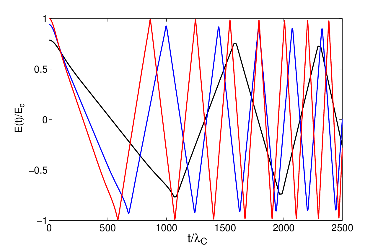
Numerical integrations. Given the parameters and of the Sauter field (12) as an initial electric field , we numerically integrate Eqs.(16-19) in the spatial region : and time interval : , where is the Compton time. The value is chosen so that the adiabatic condition (23) is satisfied, and the spatial range is determined by the capacity of computer for numerical calculations. The electric field strength is chosen around the critical value , so that the semiclassical pair-production rate (22) can be approximately used. Actually, and are attributed to the characteristics of external ultra-strong electric fields established by either experimental setups or astrophysical conditions.
In Figs. 1 and 2, we respectively plot the time- and space-evolution of the total electric fields (21) as functions of and at three different spatial points and times. As discussed in Figure captions, numerical results show the properties of the electric field wave propagating in the plasma of oscillating electron-positron pairs, as described by the wave equation (24). This electric field wave propagates along the directions in which external electric field-strength decreases. The wave propagation is rather complex, depending on the space and time variations of the net charge density and current density , as shown in Figs. 4-5. The net charge density oscillates (see Figs. 3 and 4) proportionally to the field-gradient (20) and at the center the charge density and field-gradient are zero independent of time evolution (see Fig. 4). However, the total charge of pairs must be zero at any time, as required by the neutrality. The electric current alternating in space and time follows the space and time evolution of the electric field see Eq. (19), as shown in Figs. 5 and 6.
We recall the discussions of the plasma oscillations in the case of spatially homogeneous electric field without boundary [22, 23]. Due to the spatial homogeneity of electric fields and pair-production rate (1), the number-densities (2), “averaged” velocities (3) and energy-momenta (8) are spatially homogeneous so that the charge density (15) identically vanishes and current (14) . All spatial derivative terms in Eqs. (16-18) and Eq. (24) vanish and Eq. (20) becomes irrelevant. As results, the plasma oscillations described is the oscillations of electric fields and currents with respect time at each spatial point, and the electric field has no any spatial correlation and does not propagate.
In contrary to the plasma oscillation in homogeneous fields, the presence of such field-propagation in inhomogeneous fields is due to: (i) non-vanishing field-gradient (20) and net charge-density (15), as shown in Figs. 3 and 4, give the spatial correlations of the fields at neighboring points; (ii) the stronger field-strength, the larger field-oscillation frequency is, as shown in Fig. 1; (iii) at the center the field-strength is largest and the field-oscillation is most rapid, and the field-oscillations at points are slower and in retard phases, as shown in Fig. 2. The point (i) is essential, the charge density oscillates (see Figs. 3 and 4) proportionally to the field-gradient Eq. (20) and at the center the charge density and field-gradient are zero independent of time evolution (see Fig. 4). Such field-propagation is reminiscent of the drift motion of particles driven by a field-gradient ( “ponderomotive”) force, which is a cycle-averaged force on a charged particle in a spatially inhomogeneous oscillating electromagnetic field [38].


Radiation fields. As numerically shown in Fig. 1-6, the propagation of the electric field wave inside the region is rather complex, due to th high non-linearity of wave equation (24). Nevertheless, the electromagnetic radiation fields and far away from the region are completely determined and could be experimentally observable. At the space-time point () of an observer, the electromagnetic radiation fields and , emitted by the variations of electric charge density and current-density in the region and time , are given by [37]
| (25) | ||||
| (26) |
where the subscript “” indicates , . In the radiation zone and , where is far away from the plasma oscillation region , the radiation fields (25,26) approximately are
| (27) | ||||
| (28) |
where we use the charge conservation (9) and total neutrality condition of pairs . The first terms in Eqs. (25,26) are the Coulomb-type fields decaying away as . The Fourier transforms of Eqs. (27) and (28) are
| (29) | ||||
| (30) |
where the wave number and the numerical integration (30) is carried out overall the space-time evolution of the electric current (see Figs. 6 and 5). For definiteness we thinks of the oscillation currents occurring for some finite interval of time or at least falling off for remote past and future times, so that the total energy radiated is finite, thus the energy radiated per unit solid angle per frequency interval is given by [37]
| (31) |
The squared amplitude as a function of gives the spectrum of the radiation (see Fig. 7), which is very narrow as expected with a peak locating at KeV for , consistently with the plasma oscillation frequency (see Fig. 1). The energy-spectrum and its peak are shifted to high-energies as the initial electric field-strength increases, and the relation between the spectrum peak location and the electric field-strength is shown in Fig. 8. In addition, the energy-spectrum and its peak are also shifted to high-energies as the temporary duration of plasma oscillations increases (see Fig. 1). In calculations, the temporary duration is chosen, not only to satisfy the adiabaticity condition Eq. (23) [39], but also to be in the time duration when the oscillatory behavior is distinctive (see Figs. 1,4,6), since the oscillations of pair-induced currents damp and pairs annihilate into photons [22]. The radiation intensity (31) depends on the strength, spatial dimension and temporal duration of strong external electric fields, created by either experimental setups or astrophysical conditions.


Conclusions and remarks. We show the space and time evolutions of pair-induced electric charges, currents and fields in strong external electric fields bounded within a spatial region. These results imply the wave propagation of the pair-induced electric field and wave-transportation of the electromagnetic energy in the strong field region. Analogously to the electromagnetic radiation emitted from an alternating electric current, the space and time variations of pair-induced electric currents and charges emit an electromagnetic radiation. We show that this radiation has a the peculiar energy-spectrum (see Fig. 7) that is clearly distinguishable from the energy-spectra of the bremsstrahlung radiation, electron-positron annihilation and other possible background events. This possibly provides a distinctive way to detect the radiative signatures for the production and oscillation of electron-positron pairs in ultra-strong electric fields that can be realized in either ground laboratories or astrophysical environments.
As mentioned in introduction, the critical electric field will be reached soon in ground laboratories and sensible methods to detect signatures of pair-productions become important. Recently, the momentum signatures of pair-production is found [40] in a time-varying electric field with sub-cycle structure. On the other hand, space-based telescopes the Swift-BAT [41], NuSTAR [42] and Astro-H [43] focusing high-energy X-ray missions, will also give possibilities of detecting X-ray radiation signature, discussed in this paper, from compact stars with electromagnetic structure.
Acknowledgements: We thank H. Keinert for helpful discussions on the wave equation (24).
References
- [1] R. Ruffini, G. V. Vereshchagin, S.-S. Xue, Phys. Rep., Vol 487, (2010) 1.
- [2] F. Sauter, Z. Phys. 69 (1931) 742.
- [3] W. Heisenberg, H. Euler, Z. Phys. 98 (1935) 714.
- [4] J. Schwinger, Phys. Rev. 82 (1951) 664.
- [5] A. Ringwald, Phys. Lett. B510 (2001) 107.
- [6] T. Tajima, G. Mourou, Phys. Rev. ST Accel. Beams 5 (2002) 031301.
- [7] S. Gordienko et al, Phys. Rev. Lett. 94 (2005) 103903.
- [8] http://www.sfel.eu
- [9] http://www.extreme-light-infrastructure.eu
- [10] D. L. Burke, et. al., Phys. Rev. Lett. 79 (1997) 1626.
- [11] V. V. Usov, Phys. Rev. Lett. 80, 230, 1997.
- [12] V. V. Usov, T. Harko , K.S. Cheng, Astrophys.J. 620 (2005) 915.
- [13] R. Ruffini, M. Rotondo , S-S Xue, Int. J. Mod. Phys. D16 (2007) 1.
- [14] M. Rotondo, J. A. Rueda, R. Ruffini , S-S Xue, arXiv:0911.4622v1 (2009).
- [15] J. A. Rueda, R. Ruffini, S-S Xue, arXiv:0911.4622v1 (2009).
- [16] V. Popov, M. Rotondo, R. Ruffini , S-S Xue, arXiv:0903.3727v1 (2009).
- [17] Y. Kluger, J. M. Eisenberg, B. Svetitsky, F. Cooper , E. Mottola, Phys. Rev. Lett. 67 (1991) 18; Phys. Rev. D45 (1992) 4659.
- [18] F. Cooper , E. Mottola, Phys. Rev. D40 (1989) 456.
- [19] T. S. Biro, H. B. Nielsen , J. Knoll, Nucl. Phys. B245 (1984) 449.
- [20] G. Gatoff, A.K. Kerman , T. Matsui, Phys. Rev. D36 (1987) 114.
- [21] F. Cooper, J. M. Eisenberg, Y. Kluger, E. Mottola, B. Svetitsky, Phys. Rev. D48 (1993) 190.
- [22] R. Ruffini, L. Vitagliano, S.-S, Xue, Phys. Lett. B 559 (2003) 12.
- [23] R. Ruffini, G. V. Vereshchagin, S.-S, Xue, Phys. Lett. A, 371 (2007) 399.
- [24] A. Ringwald, Phys. Lett. B510 (2001) 107.
- [25] S. S. Bulanov, N. B. Narozhny, V. D. Mur , V. S. Popov, ZhETF 129 (2006) 14 [JETP 102 (2006) 9].
- [26] D. B. Blaschke, A. V. Prozorkevich, C. D. Roberts, S. M. Schmidt , S. A. Smolyansky, Phys. Rev. Lett. 96 (2006) 140402.
- [27]
R. Schutzhold, H. Gies , G. V. Dunne, Phys. Rev. Lett. 101 (2008) 130404; Phys. Rev. D80 (2009) 111301(R);
F. Hebenstreit, R. Alkofer, H. Gies, Phys. Rev. D78 (2008) 061701. - [28] R. Ruffini, L. Vitagliano, S.-S. Xue, Phys. Lett. B573 (2003) 33.
- [29] H. Kleinert, R. Ruffini, S.-S. Xue, Phys. Rev. D. 78 (2008) 025001.
- [30] S. Weinberg, Gravitation and Cosmology ISBN 0-471-92567-5, John Wiley & Sons, 1972.
- [31] K. Kajantie, T. Matsui, Phys. Lett. B164, 373, 1985.
- [32] For an electric field , the number-density of electron-positron pairs is small and the pressure of pairs can be neglected. While for an over electric field , the number-density of pairs is large and the collisions and annihilation of pairs into photons are important, leading to the energy equipartition of electron, positrons and photons. In this case, the pressure, effective temperature and equation of state have to be considered.
- [33] W. Greiner, B. Müller, J. Rafelski, Quantum Electrodynamics of Strong Fields (Springer-Verlag, Berlin, 1985).
- [34] A.A. Grib, S.G. Mamaev, V.M. Mostepanenko, Vacuum Quantum Effects in Strong External Fields (Atomizdat, Moscow, 1980).
- [35] E. Brezin , C. Itzykson, Phys. Rev. D2 (1970) 1191.
- [36] V. S. Popov, JETP Lett. 13 (1971) 185; JETP Lett. 18 (1973) 255.
- [37] J. D. Jackson, Classical Electrodynamics, 3rd (1998), John Wiley & Sons, Inc. ISBN 978-0-471-30932-1.
- [38]
H. A. H. Boot, R. B. R. -S. Harvie,
Nature 180 (1957) 1187;
A. V. Gaponov, M. A. Miller, Sov. Phys. JETP 7 (1958) 168;
T. W. B. Kibble, Phys. Rev. Lett. 16 (1966) 1054;
F. A. Hopf et. al., Phys. Rev. Lett. 37 (1976) 1342. - [39] We check the two cases and , and find for the first oscillation and respectively. As can be seen for the Fig. 1 the frequencies of pair-oscillations increase with time which means the parameter becoming smaller. Eventually it may reach unity so the formula (22) becomes inapplicable.
- [40] F. Hebenstreit, R. Alkofer, G. V. Dunne , H. Gies, Phys. Rev. Lett. 102 (2009) 150404
- [41] http://swift.gsfc.nasa.gov/docs/swift/swiftsc.html
- [42] http://www.nustar.caltech.edu/
- [43] http://astro-h.isas.jaxa.jp/