Inference with Transposable Data: Modeling the Effects of Row and Column Correlations

We propose to study row and column correlations through a simple matrix decomposition model based on the matrix-variate normal. We motivate the use of this distribution through the example of microarrays.

In microarray data, the genes are often assumed to follow a multivariate normal distribution with the arrays independent and identically distributed. Since we aim to study the effects of array correlations, we need a parametric model that has the flexibility to model either array independence or various array correlation structures. To this end, we turn to the mean-restricted matrix-variate normal introduced in Allen and Tibshirani (2010). (We also note that Efron (2009) proposes the matrix-variate normal as a model for microarrays). This distribution, denoted as $\X\sim N_{m,n}(\nu,\mu,\Sig,\Delt)$, has separate mean and covariance parameters for the rows, $\nu\in\Re^{m}$ and $\Sig\in\Re^{m\times m}$, and columns, $\mu\in\Re^{n}$ and $\Delt\in\Re^{n\times n}$. Thus, we can model array correlations directly though the covariance matrix $\Delt$. If the matrix is transformed into a vector of length $np$, we have that $\mathrm{vec}(\X)\sim N(\mathrm{vec}(\M),\Omeg)$, where $\M=\nu\mathbf{1}^{T}_{(n)}+\mathbf{1}_{(m)}$ and $\Omeg=\Delt\otimes\Sig$. Also, the commonly used multivariate normal is a special case of the distribution. If $\Delt=\mathbf{I}$ and $\mu=\mathbf{0}$, then $\X\sim N(\nu,\Sig)$. In fact, all marginal models of the matrix-variate normal are multivariate normal, meaning that both the genes and arrays separately are multivariate normal. Further properties of this distribution are given in Allen and Tibshirani (2010).

In our matrix decomposition model, we will assume that the data, $\X$, has $m$ rows and $n$ columns. We define the overall row means as $\nu\in\Re^{m}$ and column means as $\mu\in\Re^{n}$. The covariance of the rows is $\Sig\in\Re^{m\times m}$ and the covariance of the columns is $\Delt\in\Re^{n\times n}$. Then, we decompose the data into a mean, signal, and correlated noise matrix as follows.

Thus, $\X-\Smat\sim N_{m,n}(\nu,\mu,\Sig,\Delt)$, meaning that after removing the signal, the data follows a mean-restricted matrix-variate normal distribution.

For the example of the two-class microarray, we let there be $n_{1}$ arrays in class one, with indices denoted by $\mathcal{C}_{1}$, and $n_{2}$ in class two, $\mathcal{C}_{2}$. (For simplicity of notation, we assume that the first $n_{1}$ arrays are in class one and the last $n_{2}$ arrays are in class two.) The class signals, or the gene means for each class are defined as $\psi_{1}\in\Re^{m}$ and $\psi_{2}\in\Re^{m}$. Then, the signal matrix, $\Smat$, can be written as follows.

There are several remarks to make regarding this model. First, prior to analyzing data, it is common to standardize the rows. Sometimes this two-way data is doubly-standardized, or both the rows and columns are iteratively scaled (Efron, 2009; Olshen and Rajaratnam, 2010). Here, we center both the rows and columns through the mean matrix $\M$, but do not directly scale them. Instead, we allow the diagonals of the covariance matrices of the rows, $\Sig$, and columns $\Delt$, to capture the differences in variablities. Thus, our model keeps the mean and variances separate in the estimation process.

In this section, we study the effect of column correlations on the theoretical null distribution of two-sample test statistics computed for a single row of the data matrix. More specifically, we calculate the distributions of test statistics under our matrix decomposition model instead of the typical two-sample framework where samples are drawn independently from two populations. This corresponds to considering a single test for differential expression of gene $i$ between the two classes.

In the familiar two-sample hypothesis testing problem, we have a vector $\x=[\x_{1}\hskip 5.69054pt\x_{2}]$ with $\x_{1}$ of length $n_{1}$ and $\x_{2}$ of length $n_{2}$ where the elements of each vector are $x_{1,i}\displaystyle\simiid^{iid}N(\psi_{1},\sigma^{2})$ and $x_{2,i}\displaystyle\simiid^{iid}N(\psi_{2},\sigma^{2})$. We wish to test whether there is a shift in means between the two classes, namely

Throughout this paper, we will assume that the variances $\sigma^{2}$ are equal between the two classes, a common assumption in microarrays.

If the variance, $\sigma^{2}$ is known, we have the familiar two-sample $Z$-statistic,

where $\bar{x}_{k}=\frac{1}{n_{k}}\sum_{i=1}^{n_{k}}x_{i}$ and $c_{n}=\frac{1}{n_{1}}+\frac{1}{n_{2}}$.

Now, going back to our matrix decomposition model, we wish to know the distribution of the $Z$-statistic for each row when there are column correlations.

In terms of the decomposition (1), the assumptions of Theorem 1 correspond to a row vector previously centered by $\nu$ and $\mu$, with signal $[\psi_{1}\mathbf{1}_{(n_{1})}\hskip 5.69054pt\psi_{2}\mathbf{1}_{(n_{2})}]$, column covariance $\Delt$, and row variance $\sigma^{2}$, the diagonal element of $\Sig$. For microarrays, the result states that when the columns (arrays) are correlated, the variance of the $Z$-statistic is inflated or deflated by $\eta$, a function of the column covariance. Notice that if $\Delt=\mathbf{I}$, $\eta=c_{n}$ and the variance of $Z$ is one. If there is only column correlation within the two classes we have the following result.

In both of the previous results, we assumed that the row variance, $\sigma^{2}$ was known. However, in most microarray experiments this is not known and must be estimated. With $\sigma^{2}$ unknown, for testing the hypothesis (2), the two-sample $t$-statistic is used.

with $c_{n}$ and $\bar{x}_{k}$ as previously defined. Under the null hypothesis, $T\sim t_{(n-2)}$, while under the alternative, $T\sim t(\delta)_{(n-2)}$, a non-central $t$ distribution with non-centrality parameter $\delta=(\psi_{1}-\psi_{2})/(\sigma\sqrt{c_{n}})$.

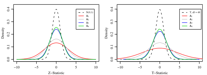
When there are column correlations as in the assumptions of Proposition 1, however, the distribution of $T$ does not have a closed form. (The square of the pooled sample standard deviation is no longer distributed as a Chi-squared random variable and the numerator and denominator of $T$ are not independent.) Hence, we explore the effects of column correlations on the $T$-statistic through a small simulation study. Data is simulated according to the assumptions of Theorem 1 with $n=50$ columns with $n_{1}=n_{2}=25$ in each class. Four structured covariance matrices were used to assess the $Z$ and $T$-statistics under the column correlations scenarios, as given below.

• •

  $\Delt_{1}:\Delt_{1,ij}=0.9^{|i-j|}$.

• •

  $\Delt_{2}$: Blocked diagonal with blocks of size 10. Within each block, $\Delt_{2,ij}=0.9^{|i-j|}$.

• •

  $\Delt_{3}:\Delt_{3,ij}=0.5^{|i-j|}$.

• •

  $\Delt_{4}$: Blocked diagonal with blocks of size 10. Within each block, $\Delt_{4,ij}=0.5^{|i-j|}$.

Figure 2 reveals the effect of column correlations on the distributions of $Z$ and $T$. We see that column correlations can cause dramatic over-dispersion of the test statistics compared to their theoretical null distribution. This is a possible explanation to the over-dispersion seen in the real microarray examples of Figure 1. Compared to the variance of the $Z$-statistic, the $T$-statistic appears to be even more affected by column correlations. This is confirmed in Table 1 where we present the variances of the $Z$-statistic calculated by Theorem 1 and the variances of the $T$-statistic estimated by Monte Carlo simulation. Indeed, small amounts of correlation in the columns can cause a dramatic increase in the variance of the $T$-statistic.

In this section, we have shown how the distribution of $T$ and $Z$-statistics behave when columns or arrays are correlated. When analyzing microarrays, however, many have advocated using a non-parametric method, estimating the null distribution by permutations Ge et al. (2003); Storey and Tibshirani (2003); Tusher et al. (2001). For the two-class microarray, one would permute the class labels and calculate the $T$-statistic for each permutation. These permutations form a null distribution, as under the null hypothesis (2), the class means are the same. Thus, each permutation of the labels is equally likely. When the arrays are correlated, however, this assumptions fails. Each permutation of the columns is not equally likely under the null due to the array covariance structure. While we do not explore the behavior of the permutation nulls further in this section, we include permutation-based methods from Storey and Tibshirani (2003) in our simulation study in the following section.

A common error measure for controling the number of false positives in microarrays is the False Discovery Rate (FDR). This is the expectation of the False Discovery Proportion (FDP): let $V$ be the number of false positives and $R$ be the total number of rejections, then $q=FDR=\mathrm{E}(V/R|R>0)$. Typically, investigators seek to control the FDR at $q=0.1$, meaning that on average 10% of rejections are false.

The step-up method of Benjamini and Hochberg (1995) is one of the most widely used methods for controling the FDR. Benjamini and Yekutieli (2001) have shown that this method controls the FDR under types of positive dependence, specifically positive regression dependence, and Sarkar (2008) has relaxed this assumption to slightly broader forms of positive dependence. This may not be appropriate for all types of transposable data, especially microarrays where we expect some negative correlations between genes. Alternatively, Benjamini and Yekutieli (2001) have shown that dividing the thresholds in the step-up procedure by a constant controls the FDR under arbitrary dependencies.

Another commonly used method to control the FDR is based on re-sampling or permutation distributions (Ge et al., 2003; Storey, 2002; Tusher et al., 2001; Yekutieli and Benjamini, 1999). Theoretically, these methods are only known to control the FDR asymptotically under types of weak dependence, which encompasses forms of local dependence such as finite blocks (Storey et al., 2004). Thus, there could be many transposable data sets in which the row variables do not satisfy these dependence structures. (We also note that applying the step-up method to the permutation-adjusted $p$-values is equivalent to the direct FDR estimation via re-sampling (Storey et al., 2004)).

Also, to directly account for correlations, Efron (2004); Efron (2007) proposed a method to fit an empirical null to the data. One can then estimate the local FDR and then the FDR by averaging the local FDR over the tail regions.

We study the effects of both row and column correlations on standard statistical methodology used for large-scale inference through a simulation study based on our matrix decomposition model. We compare FDR estimates of four types of FDR-controlling procedures to the true false discovery proportion (FDP). The four methods we compare are the step-up method of Benjamini and Hochberg (1995), the step-up method for control under arbitrary dependence of Benjamini and Yekutieli (2001), the permutation-based method of Storey and Tibshirani (2003), and the method based on the empirical null and local FDR’s of Efron (2007). The two-sample $t$-statistic was used for all methods with $p$-values computed by comparing it to the $t_{(n-2)}$ distribution for the step-up procedures. We used 1000 permutations for the permutation-based method. The defaults in the localfdr package available on CRAN, the R language repository. These defaults fit the null distribution as a natural spline with seven degrees of freedom, for the empirical null-based method.

Our simulation study is structured as follows. The data is simulated under the matrix decomposition model (1) and is of size 250 by 50. The first 50 rows are non-null with a two-class signal matrix given by $\psi_{1,1:25}=0.5$, $\psi_{1,26:50}=-0.5$, $\psi_{2,1:25}=-0.5$, $\psi_{2,26:50}=0.5$ and the last 200 elements of $\psi_{1}$ and $\psi_{2}$ equal to zero. We consider two types of row covariances, $\Sig_{1}$ with all positive correlations satisfying the positive regression dependence assumption of (Benjamini and Yekutieli, 2001), and $\Sig_{2}$ with both positive and negative correlations. Both of these row covariances are block diagonal. We simulate data under three column covariances, with the first being the identity, or no column correlations. The others, $\Delt_{1}$ and $\Delt_{2}$ reflect a local and a class effect, respectively. These simulation covariances are summarized below.

• •

  $\Sig_{1}$: Blocked diagonal with blocks of size 10. Within each block, $\Sig_{1,ij}=0.9^{|i-j|}$.

• •

  $\Sig_{2}$: Blocked diagonal with blocks of size 10. Within each block, $\Sig_{2,ij}=(-0.9)^{|i-j|}$.

• •

  $\Delt_{1}$: Blocked diagonal with blocks of size 10. Within each block, $\Delt_{1,ij}=0.5^{|i-j|}$.

• •

  $\Delt_{2}$: Blocked diagonal with blocks of size 25. Within each block, $\Delt_{2,ij}=0.5^{|i-j|}$.

We present plots of the true FDP verses the number of hypotheses rejected for the four methods for one realization of each of the six simulation scenarios in Figure 3. We note that the lines above the true FDP curve denote conservative FDR estimates. In Table 2, we report the true and estimated false discovery proportions (FDP) when fixed numbers of hypotheses are rejected (40, 45, 50, 55 and 60 tests). Results are averaged over ten simulations with the standard error also reported.

This simulation study reveals several interesting results. First, dependencies among the rows do not seem to effect FDR estimation with the four multiple testing procedures. When, $\Delt=\mathbf{I}$ as in simulations (a) and (b), the methods generally conservatively estimate the true FDP. This is noteworthy since besides the method of Benjamini and Yekutieli (2001), there are limited theoretical results supporting FDR control under various dependencies.

When there are even moderate correlations between columns, simulations (c) through (f), the four methods give poor estimates of the FDR. The step-up method and the permutation-based method perform similarly. They both give extremely conservative estimates of the FDP when there is either a local or a class effect among the columns. Thus, when using these methods for controlling the FDR at $q=0.1$, for example, one would reject less than 45 genes, when in reality one should be permitted to reject around 55 genes. We also see that while the method of Benjamini and Yekutieli (2001) controls the FDR are arbitrary dependencies, in practice this method is much too conservative for general use. On the other hand, the empirical null-based method of Efron (2007) performs inconsistently.

Overall, the results of this simulation study reveal that dependencies among rows do not seem to effect the performance of the multiple testing procedures. On the other hand, the theoretical results of Section 2.2 are confirmed: dependencies among the columns are extremely problematic when conducting large-scale inference.

The Transposable Regularized Covariance Model (TRCM) allows us to estimate a non-singular row and column covariance matrix by maximizing a penalized log-likelihood of the matrix-variate normal distribution (Allen and Tibshirani, 2010). The model places a strictly convex penalty on the inverse covariances, or concentration matrices, of the rows and columns. For estimating the covariances in this context, we propose to use a sparsity-inducing penalty, an $L_{1}$ penalty, on the concentration matrices. Following from the matrix decomposition model, (1), if we let $\N$ be the noise matrix remaining after removing the means and the signal in the data, then the penalized log-likelihood is as follows.

where $||\Delti||_{1}=\sum_{i=1}^{n}\sum_{j=1}^{n}|\Delti_{ij}|$ and $\lambda$ is a penalty parameter that must be estimated.

We motivate the use of (6) first by discussing practical considerations. As the columns of the data matrix are usually There are several advantages assumed to be independent, $\Delt=\mathbf{I}$, this should be our default position. By placing an $L_{1}$ penalty on $\Delti$, our model encourages sparsity in the off-diagonal elements of $\Delt$. Also, notice that we have one penalty parameter, $\lambda$, that is modulated by the dimension of the rows and columns. (We note that the penalty parameter, $\lambda$, can be selected by cross-validation). Thus, the evidence of a partial correlation among columns must be strong relative to the correlations among the rows for an off-diagonal element of $\Delti$ to be estimated as non-zero. Secondly,specifically for microarrays, it seems reasonable to assume that the covariances among the genes is sparse, since biologically genes are likely only to be correlated with genes in the same or related pathways.

We also pause briefly to discuss the theoretical rationale for using $L_{1}$ penalties, instead of, for example, $L_{2}$ penalties. Recall that covariance solutions to the TRCM model with $L_{2}$ penalties have eigenvectors that are equal to the left and right singular vectors of the data (Allen and Tibshirani, 2010). Thus, the singular vectors of the data would remain the same when sphering with these estimates. In high-dimensional settings, however, it is well established that eigenvectors of empirical covariances are inconsistent (Johnstone and Lu, 2004), and thus, sphering by the $L_{2}$ covariance estimates seems ill-advised. While the consistency of $L_{1}$ TRCM estimates has not been established, there are consistency results for multivariate covariance estimation with an $L_{1}$ penalty. Rothman et al. (2008) show convergence of the multivariate covariance estimate in the Frobenius norm and more importantly for the correlation estimate in the operator norm which implies convergence of the eigenvectors (El Karoui, 2008). These results reveal some of the possible theoretical advantages of using $L_{1}$ penalties to estimate the covariances.

Based on the matrix decomposition model, (1), we present a method of de-correlating or sphering the data so that the rows and columns are approximately independent. This sphered data can then be used with standard multiple testing procedures to identify significant row variables. Given a data matrix $\X$ with $m$ rows and $n$ columns, we present our sphering algorithm in Algorithm 1.

The Sphering Algorithm simply estimates the means and signal according to the matrix decomposition model (1) and then estimates the correlation structure among the rows and columns in the remaining noise. The TRCM covariance estimates, $\hat{\Sig}$ and $\hat{\Delt}$ are used to de-correlated the noise. Here, $\hat{\Sig}^{-1/2}$ is the matrix square root of $\hat{\Sig}^{-1}$ and $\hat{\Delt}^{-1/2}$ of $\hat{\Delt}$. (We use the symmetric square root defined by the following. Let $\hat{\Sig}^{-1}=\mathbf{P}\Lambda\mathbf{P}^{T}$ be the eigenvalue decomposition of $\hat{\Sig}^{-1}$, then the symmetric matrix square root is given by $\hat{\Sig}^{-1/2}=\mathbf{P}\Lambda^{1/2}\mathbf{P}^{T}$.) Adding the signal back into this sphered noise, we obtain $\tilde{\X}$ which we call the sphered data. One can use this de-correlated data to find significant row variables.

Now, we investigate some of the theoretical properties of the sphered data for the two-class problem introduced in Section 2.2. The sphered data, $\tilde{\X}$ has the following properties.

Thus, the class signal remains the same between $\X$ and $\tilde{\X}$, and the covariance structure is all that changes. By sphering the noise, the noise of each row in $\tilde{\X}$ becomes a linear combination of the noise in the other rows.

We now study how sphering the data affects the $Z$ and $T$ statistics from Section 2.2. First, the $Z$-statistic does not change with sphering. The numerator of both the $Z$ and $T$ statistic, $\bar{x}_{1}-\bar{x}_{2}$ is given by $\hat{\psi}_{1}-\hat{\psi}_{2}$, the components of the estimated signal matrix $\hat{\Smat}$. The denominator of the $T$-statistic, namely $s_{x_{1},x_{2}}$, the estimate of the noise, however, changes with sphering. Recall that in Section 2.2, we discussed how the $T$-statistic does not have a closed form distribution when there are column correlations. After sphering the data, however, the $T$-statistic on the sphered data follows a scaled $t$ distribution under certain conditions. This is given by the following result.

Using our sphering algorithm, we obtain test statistics that follow known distributions when the sphered column covariance, $\tilde{\Delt}$ is the identity. If $\tilde{\Delt}$ is instead a diagonal matrix, then a simple scaling of the columns will give the above result. Notice that if the original data, $\X$, has no column correlations, $\Delt=\mathbf{I}$, and $\tilde{\sigma}_{i}=\sigma_{i}$, then $T$ and $\tilde{T}$ both follow a $t$ distribution with $n-2$ degrees of freedom. Thus, if the data originally follows the correct theoretical null distribution, then sphering the data does not change its null distribution. Also, if the sphered rows are independent, $\tilde{\Sig}=\mathbf{I}$, or approximately independent, then the statistics, $T_{i}$ are independent or approximately independent. We also note that we can often assume that $\tilde{\sigma}_{i}=\sigma_{i}$, thus eliminating that coefficient ratio from the distribution. This is especially a reasonable assumption if the rows are scaled prior to applying the sphering algorithm.

Our results in Proposition 2 hold if the sphered column covariance $\tilde{\Delt}$ is the identity or diagonal. The TRCM model, however, estimates sparse penalized row and column covariances. These penalized estimates will not capture the full covariances, but will instead estimate the major correlations. Thus, in practice, $\tilde{\Delt}$ and $\tilde{\Sig}$ are not likely to be exactly the identity. We have observed in simulations, however, that $\tilde{\Delt}$ is often diagonal or nearly diagonal, and thus the theoretical results are appropriate.

When calculating $p$-values for $\tilde{T}$ based on the distribution given in Proposition 2, we must know the value of $\eta$ which depends on the original column covariance $\Delt$. One could estimate this from $\hat{\Delt}$, but since the TRCM framework estimates penalized covariances, an estimate, $\hat{\eta}$, based on $\hat{\Delt}$ will underestimate the population $\eta$. Hence to obtain the null distribution of the $\tilde{T}$-statistics, we have opted to scale $\tilde{T}$ by the variance of the central portion of the observed distribution of the test statistics. This procedure is outlined in Algorithm 2 where $\rho_{\alpha}(x)$ denotes the $\alpha^{th}$ quantile of $x$. and $I()$ is the indicator function.

We scale by the central portion of the $\tilde{T}$-statistics so that the statistics can be tested against the $t_{(n-2)}$ distribution. Notice that if all of the test statistics are null and $\pi_{0}=1$ then, central-matching the variances reduces to scaling the $\tilde{T}$-statistics. Since under the assumptions of Proposition 2, only the null $\tilde{T}_{i}$ follow a scaled $t$-distribution, we do not want statistics corresponding to non-null tests to contaminate the variance estimates. Thus, we recommend using a conservative estimate of $\pi_{0}$, such as 0.8 or 0.9 for microarrays.

By applying our sphering algorithm, we directly account for correlations among the rows and columns. This results in test statistics that more closely follow both their theoretical nulls and the theoretical assumptions under which common multiple testing procedures are known to control the false discovery rate.

In all of these simulations, the data, $\X$ is simulated from the matrix decomposition model (1) with $m=250$ rows and $n=50$ columns. The first 50 rows are non-null given by $\psi_{1,1:25}=0.5$, $\psi_{1,26:50}=-0.5$, $\psi_{2,1:25}=-0.5$, $\psi_{2,26:50}=0.5$ and the last 200 elements of $\psi_{1}$ and $\psi_{2}$ equal to zero.

In Table 3, we present results on a subset of the simulations from our simulation study in Section 3.2. The remaining simulation study results are given in Appendix A. The results in Table 3 show that de-correlating the data matrix yields improvements in 1) statistical power and 2) estimation of the FDR. We briefly illustrate this by examining a specific example from Table 3.2. Take the simulation with parameters $\Sig_{1}$, $\Delt_{1}$ and look at the results with 55 tests rejected. We notice that the true FDP for the data pre-processed by the standard method is 0.111 whereas it is lower, 0.105, on the data that was sphered. This results from a favorable re-ordering of the test statistics that gives a higher statistical power, one minus the true FDP. Next, notice that the FDR estimates for the step-up and permutation-based methods are 0.426 and 0.43 respectively for the un-sphered data. These estimates are overly conservative, as the true FDP is 0.111. After sphering, however, the FDR estimates are 0.124 and 0.125 which are much closer to the true FDP of 0.105. Hence, sphering also improves FDR estimation.

Sphering the data as a pre-processing step to multiple testing procedures has many advantages. First in microarrays, the higher statistical power that results from a re-ordering of test statistics is important to scientists who desire the top ranked genes from one microarray study to translate to the top genes in another study. Also, while sphering leads to improvements in FDR estimation, it is still a slightly conservative estimate, as desired, for the true FDP. As with the simulation study, we find that the empirical null based method of Efron (2007) gives an inconsistent estimate of the FDR as it is both a conservative and liberal estimate for differing numbers of rejected tests.

We also wish, however, to test the performance of our sphering algorithm on data with dependencies more similar to real microarray data. Thus, we build a second simulation study based upon the empirical covariances of the “Cardio” and the “Leukemia” microarrays. For each of the ten repetitions, we sample 250 genes and 50 arrays at random from each microarray. Let $i\in\mathcal{I}$ and $j\in\mathcal{J}$, be the sampled sets of the genes and arrays respectively, and assume $\X$ is the centered data matrix. We then calculate the empirical covariances, $\Delt_{MLE}=\sum_{i\in\mathcal{I}}\sum_{i^{\prime}\in\mathcal{I}}X_{i}^{T}X_{i^{\prime}}/m$, and $\Sig_{MLE}=\sum_{j\in\mathcal{J}}\sum_{j^{\prime}\in\mathcal{J}}X_{j}X_{j^{\prime}}^{T}/n$. The data is simulated from the mean-restricted matrix-variate normal with $\X\sim N(\left[\psi_{1}\hskip 5.69054pt\psi_{2}\right],\mathbf{0},\Sig_{MLE},\Delt_{MLE})$. Hence, the simulated data follows the observed covariance of the “Cardio” and “Leukemia” studies. Example images and FDR curves from this simulation are given in Figure 4 as well as the simulation results in Table 4.

The results of the structured covariance study, namely improvements in statistical power and FDR estimation, are confirmed on these microarray-based simulations. There are also some specific notes to make regarding these simulations. First in Table 4, notice that using un-sphered data the FDR is overestimated on the “Cardio” simulations and underestimated on the “Leukemia” simulations. This is confirmed by the example giving the full FDR curves in Figure 4. After sphering, however, we see that the FDR estimates for both simulations are still conservative, but much closer to the true FDP. We note that all ten repetitions of the “Cardio” simulation estimated both $\hat{\Sig}$ and $\hat{\Delt}$ to be non-diagonal. This means that even after accounting for the correlations among the genes, there still appear to be significant correlations among the arrays. In the “Leukemia” simulation, however, $\hat{\Delt}$ was estimated to be diagonal in all ten simulations. Thus, the correlations among the genes may be driving the over-dispersion seen in the $t$-statistic distributions of Figure 1.

Thus, from these simulations based on our matrix decomposition model, we see that sphering the data as a pre-processing step greatly improves statistical power and false discovery rate estimation.

We now evaluate the performance of our method using simulations based on models other than the matrix-variate normal, namely a latent variable model and a random effects model. In these simulations we will not only compare our sphering method to the standard method, but also to the surrogate variable analysis method of Leek and Storey (2008). We first compare this method and model’s properties to our sphering algorithm and matrix decomposition model, and then compare these methods numerically.

To account for possible latent variables in a multiple testing framework, Leek and Storey (2008) propose a matrix model and the surrogate variable analysis (SVA) method. They propose the model for the data $\X\in\Re^{m\times n}$, $\X=\mathbf{B}\Smat+\mathbf{\Gamma}\mathbf{G}+\mathbf{U}$ where $\Smat$ is a signal matrix, $\mathbf{G}\in\Re^{d\times n}$ for $d<n$ is the latent variable matrix, $\mathbf{U}\in\Re^{m\times n}$ is independent noise and $\mathbf{B}$ and $\mathbf{\Gamma}\in\Re^{m\times d}$ are coefficients to be estimated. This model is similar in nature to our matrix decomposition model (1). If we assume $\X$ has been previously centered, using the notation of the latent variable model, we can write (1) as $\X=\B\Smat+\Sig^{\frac{1}{2}}\mathbf{U}\Delt^{\frac{1}{2}}$. Thus, our model accounts for structure within the data through the row and column covariances $\Sig$ and $\Delt$, whereas their method estimates the structure through $\mathbf{G}$ and assumes the noise is additive. Assuming that the latent variable model or our model is correct, applying the respective algorithms results in approximately independent $p$-values. Also similar to our method, SVA can change the rankings of the test statistics. Unlike SVA, however, our model and sphering algorithm directly capture and account for possible correlations among the columns as well as the rows.

We simulate data from a latent variable model taken directly from Leek and Storey (2008) as well as from a random effects model denoting a batch effect. For both models, the data is of dimension $250\times 50$, with 25 columns in each class with the following signal: The first 50 rows are non-null given by $\psi_{1,1:25}=0.5$, $\psi_{1,26:50}=-0.5$, $\psi_{2,1:25}=-0.5$, $\psi_{2,26:50}=0.5$ and the last 200 elements of $\psi_{1}$ and $\psi_{2}$ equal to zero. For the latent variable model, there are two latent variables given by $G_{ij}\displaystyle\simiid^{iid}Bern(0.5)$, coefficients $\Gamma_{ij}\displaystyle\simiid^{iid}N(0,1)$ and noise $U_{ij}\displaystyle\simiid^{idd}N(0,1)$. For the random-effects model with $K$ batches indicated by indices $I(k)$, a column of the data is given by the following: $X_{rj}=\nu+\mu_{j}+\sum_{i=1}^{2}\psi_{i}I_{(j\in\mathcal{C}_{i})}+\sum_{k=1}^{K}\beta_{k}I_{(j\in I(k))}+\epsilon$, where $\nu$, $\mu_{j}$ and $\psi_{i}$ are fixed effects, and $\beta_{k}\displaystyle\simiid^{iid}N(\mu_{k},\sigma^{2}_{k}\mathbf{I})$ independent of $\epsilon\displaystyle\simiid^{iid}N(0,\Sig_{1})$ are random effects. In our simulation, we have $\mu_{k}=[-0.5\hskip 5.69054pt-0.25\hskip 5.69054pt0\hskip 5.69054pt0.25\hskip 5.69054pt0.5]$, $\sigma^{2}=0.5$, $\Sig=\Sig_{1}$ as defined in Section 3.2 and $I(k)$ indicating batches of five columns.

In Table 5, we compare the true FDP to the estimate of the FDR via the step-up method (Benjamini and Hochberg, 1995) for the data with standard pre-processing, with sphering and with Leek and Storey (2008)’s surrogate variable analysis (SVA). The SVA method was implemented using the defaults available in the package sva from CRAN, the R language repository. For the latent variable simulation, both our sphering method and the SVA method improve the rank ordering of the test statistics resulting in higher statistical power as well as improved estimates of the FDR. In the random-effects model simulation, however, the sphering algorithm substantially outperforms the standard pre-processing and the SVA method. We illustrate this by looking at the specific case where 50 tests are rejected. For the standard pre-processing and SVA methods, the true FDP is 0.48 and 0.475 respectively, meaning that on average 25 out of the 50 rejected tests are false positives. With sphering, however, the order of the test statistics is dramatically changed leading to a true FDP of 0.102 so that on average only 5 out of 50 rejected tests are false. The FDR estimates using the step-up method are also problematic for the standard and SVA methods as 0.0196 and 0.185 are substantially below the true FDPs of 0.48 and 0.475 respectively. If these methods were used, the number of false positives would not be controlled. With sphering, however, the FDR estimate of 0.14 is much closer to the true FDP, 0.102 and is a conservative estimate, as desired.

These simulations based on models other than the matrix-variate normal reveal the robustness of our pre-processing technique. Our sphering method also compares very favorably to the surrogate variable analysis, another pre-processing method.

References

- Allen and Tibshirani (2010) Allen, G. I. and R. Tibshirani (2010). Transposable regularized covariance models with an applicaiton to missing data imputation. Ann. Appl. Statist. –(–), –.
- Benjamini and Hochberg (1995) Benjamini, Y. and Y. Hochberg (1995). Controlling the false discovery rate: A practical and powerful approach to multiple testing. Journal of the Royal Statistical Society. Series B (Methodological) 57(1), 289–300.
- Benjamini and Yekutieli (2001) Benjamini, Y. and D. Yekutieli (2001). The control of the false discovery rate in multiple testing under dependency. Annals of Statistics 29, 1165–1188.
- Efron (2004) Efron, B. (2004). Large-scale simultaneous hypothesis testing: The choice of a null hypothesis. Journal of the American Statistical Association 99, 96–104.
- Efron (2007) Efron, B. (2007). Size, power and false discovery rates. Ann. Statist. 35(4), 1351–1377.
- Efron (2009) Efron, B. (2009). Are a set of microarrays independent of each other? Ann. App. Statist. 13(3), 922–942.
- El Karoui (2008) El Karoui, N. (2008). Operator norm consistent estimation of large-dimensional sparse covariance matrices. Ann. Statist. 36(6), 2717–2756.
- Ge et al. (2003) Ge, Y., S. Dudoit, and T. P. Speed (2003). Resampling-based multiple testing for microarray data analysis. TEST 12, 1–77.
- Golub et al. (1999) Golub, T. R., D. K. Slonim, P. Tamayo, C. Huard, M. Gaasenbeek, J. P. Mesirov, H. Coller, M. L. Loh, J. R. Downing, M. A. Caligiuri, C. D. Bloomfield, and E. S. Lander (1999). Molecular classification of cancer: Class discovery and class prediction by gene expression monitoring. Science 286(5439), 531–537.
- Gupta and Nagar (1999) Gupta, A. K. and D. K. Nagar (1999). Matrix variate distributions, Volume 104 of Monographs and Surveys in Pure and Applied Mathematics. Boca Raton, FL: Chapman & Hall, CRC Press.
- Hommel (1986) Hommel, G. (1986). Multiple test procedures for arbitrary dependence structures. Metrika 33(1), 321–336.
- Johnstone and Lu (2004) Johnstone, I. M. and A. Y. Lu (2004). Sparse principal components analysis. Unpublished manuscript.
- Leek and Storey (2008) Leek, J. T. and J. D. Storey (2008). A general framework for multiple testing dependence. Proceedings of the National Academy of Sciences 105(48), 18718–18723.
- Olshen and Rajaratnam (2010) Olshen, R. A. and B. Rajaratnam (2010). Successive normalization of rectangular arrays. Ann. Statist. 38(3), 1638–1664.
- Owen (2005) Owen, A. B. (2005). Variance of the number of false discoveries. Journal Of The Royal Statistical Society Series B 67(3), 411–426.
- Qiu et al. (2005) Qiu, X., A. I. Brooks, L. Klebanov, and A. Yakovlev (2005). The effects of normalization on the correlation structure of microarray data. BMC Bioinformatics 6(120), –.
- Rothman et al. (2008) Rothman, A. J., P. J. Bickel, E. Levina, and J. Zhu (2008). Sparse permutation invariant covariance estimation. Electron. J. Stat. 2, 494–515.
- Sarkar (2008) Sarkar, S. K. (2008). On methods controlling the false discovery rate. Sankhya : The Indian Journal of Statistics 70, 135–168.
- Storey (2002) Storey, J. D. (2002). A direct approach to false discovery rates. Journal Of The Royal Statistical Society Series B 64(3), 479–498.
- Storey et al. (2004) Storey, J. D., J. E. Taylor, and D. Siegmund (2004). Strong control, conservative point estimation and simultaneous conservative consistency of false discovery rates: a unified approach. Journal Of The Royal Statistical Society Series B 66(1), 187–205.
- Storey and Tibshirani (2003) Storey, J. D. and R. Tibshirani (2003). Statistical significance for genomewide studies. Proceedings of the National Academy of Sciences 100(16), 9440–9445.
- Tusher et al. (2001) Tusher, V. G., R. Tibshirani, and G. Chu (2001). Significance analysis of microarrays applied to the ionizing radiation response. Proceedings of the National Academy of Sciences of the United States of America 98(9), 5116–5121.
- Yekutieli and Benjamini (1999) Yekutieli, D. and Y. Benjamini (1999). Resampling-based false discovery rate controlling multiple test procedures for correlated test statistics. Journal of Statistical Planning and Inference 82(1-2), 171 – 196.