Calculus on manifolds of conformal maps and CFT
Benjamin Doyon
Department of Mathematics, King’s College London
Strand, London, U.K.
email: benjamin.doyon@kcl.ac.uk
In conformal field theory (CFT) on simply connected domains of the Riemann sphere, the natural conformal symmetries under self-maps are extended, in a certain way, to local symmetries under general conformal maps, and this is at the basis of the powerful techniques of CFT. Conformal maps of simply connected domains naturally have the structure of an infinite-dimensional groupoid, which generalizes the finite-dimensional group of self-maps. We put a topological structure on the space of conformal maps on simply connected domains, which makes it into a topological groupoid. Further, we (almost) extend this to a local manifold structure based on the infinite-dimensional Fréchet topological vector space of holomorphic functions on a given domain . From this, we develop the notion of conformal -differentiability at the identity. Our main conclusion is that quadratic differentials characterizing cotangent elements on the local manifold enjoy properties similar to those of the holomorphic stress-energy tensor of CFT; these properties underpin the local symmetries of CFT. Applying the general formalism to CFT correlation functions, we show that the stress-energy tensor is exactly such a quadratic differential. This is at the basis of constructing the stress-energy tensor in conformal loop ensembles. It also clarifies the relation between Cardy’s boundary conditions for CFT on simply connected domains, and the expression of the stress-energy tensor in terms of metric variations.
12 June 2012
1 Introduction
Thanks to two-dimensional conformal covariance, correlation functions in conformal field theory (CFT) transform, under conformal maps, in simple ways (see for instance [1, 2, 3]). Although this conformal symmetry is useful, it is not by itself powerful enough to give rise to the large machinery of CFT and the multitude of nontrivial results. In order to do so, one must consider some locality principles of quantum field theory, which point to the existence of quantum fields whose own correlation functions are holomorphic functions of the position. It is such holomorphic quantum fields like the stress-energy tensor, with their special analytic properties, that form the basis for rigorous algebraic constructions of CFT (for instance, vertex operator algebras and representations [4]). This paper is the first part of a work aimed at understanding these infinitesimal “local conformal symmetries” through a geometric framework of derivatives with respect to conformal maps. Here we develop some basic notions of first derivatives in general, and show that certain fundamental aspects of CFT on simply connected domains, having to do with the stress-energy tensor, arise from studying such derivatives without the need for an underlying quantum field theory structure. We then apply the general formalism to CFT correlation functions on simply connected domains, where the stress-energy tensor is identified with a conformal derivative.
1.1 Main idea
Since correlation functions in CFT are conformally covariant, the only non-trivial variations are those in their conformal moduli space (this is the moduli space of the domain with punctures where local fields insertions are present). This moduli space is finite-dimensional, and one can analyze small moduli parameter variations by taking derivatives. It is well known that moduli parameter derivatives are related to the stress-energy tensor [5]. We are interested in extending such ideas to a more general context than CFT; in particular, to Schramm-Loewner evolution (SLE) (see the review for physicists [6]) and conformal loop ensembles (CLE) [7, 8, 9], where random variables are generically supported on extended regions, by opposition to local fields of CFT. In such cases, the conformal moduli space is infinite dimensional, hence one needs an infinite-dimensional analysis. Conformal derivatives provide a general framework for such an analysis. One obtains moduli space variations by making transformations that are conformal on the boundary of the domain and on the support of the random variables or local fields, but singular in some region inside the domain.
Small variations with respect to singular conformal maps were used in [10] in the context of identifying the stress-energy tensor in SLE at zero central charge (that is, at the value where conformal restriction holds). The idea of [10] is as follows. One considers a CFT correlation function of primary fields, say on the Riemann sphere, , and its image under a map , given by . If is conformal on (a Möbius map), then the image under is equal to the initial correlation function: this is conformal covariance. However, if is not conformal on , then we are making a variation in the moduli space, so the image is different. If we choose
then is not conformal on (this is essentially a Joukowsky transform). In [10], it was noticed (by a very simple and direct calculation) that the “derivative”
exactly reproduces the right-hand side of the conformal Ward identities,
This gives a geometric interpretation to the algebraic formula that identifies the holomorphic stress-energy tensor with a descendent of the identity field (the pole at in corresponds to the application of ).
The geometric properties of the Joukowsky transform lead to an interpretation of in the context of SLE [10], and this construction was generalized to (the dilute regime of) CLE [11], which has a nonzero central charge. We note that the idea of relating small singular conformal transformation to the stress-energy tensor was also discussed in a different way in [12].
In the present paper, we put these ideas in a more general and geometric context, generalizing not only to non-primary fields, but also to situations that a priori lie outside QFT considerations.
1.2 The construction
The space of simply connected domains of the Riemann sphere (of hyperbolic type), along with the conformal maps between them, forms a groupoid . We put a non-Hausdorff topology on this groupoid that correspond to a certain compact convergence of conformal maps, and that makes maps that are analytic continuation of each other inseparable. Interpreting as a tangent bundle the vector bundle based on where each fiber is the topological space of vector fields on the corresponding domain (isomorphic to the topological space of holomorphic functions), we (almost) arrive at a notion of local Fréchet manifold. We study the derivatives on this manifold at the groupoid element given by the identity map on a domain (conformal -derivatives). These derivatives are based on the notion of Hadamard derivatives on topological vector spaces. They are elements of the continuous dual of the space of holomorphic vector fields on , which are classes of quadratic differentials (on domains of the Riemann sphere) parametrized by their singularity structure in . In each class one can choose a differential almost holomorphic on the complement . We show that when there is stationarity under Möbius maps near to the identity, then it is a holomorphic differential (which we call the global holomorphic -derivative), and it coordinate-transforms under Möbius transformations of the coordinates on . Further, if there is stationarity under conformal maps on domains complementary to (essentially, whose exterior does not intersect that of ), then the global holomorphic -derivative coordinate-transforms under transformations of coordinates on corresponding to conformal maps on . When this general theory is applied to CFT, where we take conformal derivatives of correlation functions on simply connected domains, we show that identifying the stress-energy tensor in correlation functions with the conjugation of a global holomorphic derivative reproduces the conformal Ward identities and the boundary conditions of Cardy [13]. The conjugation involves an object formed by ratio of partition functions, the relative partition function, which is Möbius invariant. In particular, the one-point function of the stress-energy tensor is a global holomorphic derivative of the logarithm of the relative partition function. We argue that this is in agreement with the well-known CFT formula relating metric variations of the partition function to one-point averages of the stress-energy tensor. Our main results are expressed in the three theorems of Section 3 and the single theorem of Section 4.
We note that in the context of the CLE construction [11], the transformation and analytic properties of the global holomorphic derivative proved here are essential, as well as the fact, also proved here, that the conformal Ward identities in CFT can be expressed using this general derivative concept. It was also in the context of CLE that the one-point average of the stress-energy tensor was first identified with the global holomorphic derivative an object that can be seen as the CLE equivalent of the CFT relative partition function.
1.3 Relations with some previous works
Many previous works are related to the present one. However, we have not seen in the literature either the theorems of Section 3 or those of Section 4; nor have we seen the concept of relative partition function.
Analytic geometry of CFT. At the initial stages of the development of CFT in the physics community, there was a strong interest in understanding the geometro-analytic meaning of various aspects of CFT; in particular of the identification of the stress-energy tensor with metric variations. In the important work [5], these metric variations are naturally associated with variations of conformal structures of compact Riemann surfaces with punctures; such variations are described by Beltrami differentials , which form the tangent space in this formulation. Equation (6) of [5] states that the CFT partition function , which depends on the Riemann surface and on the choice of metric on it, satisfies
| (1.1) |
where is the infinitesimal variation of in the direction , is the one-point function of the stress-energy tensor at the point on the Riemann surface characterized by the moduli , and on both sides a particular metric has been chosen whereby the scalar curvature is constant and the volume is 1 (since is not a quadratic differential because of the conformal anomaly, this is important for the left-hand side to be well defined).
By contrast, here, conformal maps rather than conformal structures are the objects that are affected by infinitesimal variations, and such variations are described by holomorphic vector fields rather than Beltrami differentials. Equation (1.1) is to be compared with a formula that follows from Section 4:
| (1.2) |
where the correlation function is evaluated on a simply connected domain , represents a product of fields at non-coincident points away from , the contour of integration on the left-hand side is counter-clockwise in and does not surround any point , is a holomorphic function on a simply connected domain whose complement is surrounded by the contour of integration, is the associated conformal derivative, and is the relative partition function.
In principle, the result (1.2) could be deduced from an adaptation of (1.1) to the context of boundary CFT on simply connected domains with punctures (based on the formal relation ), where the punctures are the points . Further, it is likely that both formulations – variations of conformal structures and variations of conformal maps – can be connected, through the theory of quasiconformal maps. Developing this connection, however, is beyond the scope of this paper. Note that the use of infinitesimal variations of conformal maps, rather than conformal structures, seems better adapted to the application to SLE and CLE [11]. Note also our use of the relative partition function rather than the partition function, which has nicer transformation properties (Möbius invariance).
Geometry of the Virasoro group and Teichmüller theory. Differentiable manifolds of conformal maps occur in many situations, and have been related to CFT (and to string theory) in various works in the past.
The Fréchet manifold of orientation-preserving diffeomorphisms of the circle modulo rigid rotations can be seen as a set of conformal maps through conformal welding [14, 15]; also, the universal Teichmüller space is a Banach manifold of conformal maps [16]. In fact, it turns out that has a natural complex-analytic embedding into the universal Teichmüller space [17]. The universal Teichmüller space can further be represented using an open ball in the space of functions on the unit disk (the space of Beltrami differentials) [16]. Hence, there are natural relations between variations of Beltrami differentials, variations of certain conformal maps, and variations of elements in , and all these variations have interpretations through infinite-dimensional manifolds. These have been studied extensively in the literature (see e.g. [18, 15, 19, 20, 21]), and in particular in the context of SLE [22, 23, 12]. Further, the Fréchet Lie group is closely connected to CFT: it has an essentially unique central extension, the Virasoro-Bott group, whose Lie algebra is the Virasoro algebra. Combined with the concept of geometric quantization (or the orbits method in representation theory) one obtains a geometric understanding of CFT – see for instance [19, 18, 24].
In these contexts, the sets of conformal maps are proper subsets of the set of conformal maps on a fixed simply connected hyperbolic domain (in particular, there is the requirement that they have a quasi-conformal extension to the plane), and the tangent space can be seen as a proper subset of the set of holomorphic functions on this domain. Technically, our construction differs in two points: (1) our tangent space is the Fréchet space of all holomorphic vector fields, and we use the particularities of this space to obtain our precise statements (e.g. about the dual space); (2) we do not fix the domain: we consider the groupoid of hyperbolic domains, with all conformal maps between them. Hence in particular, the theorems of Section 3 have no immediate equivalent in the context of the universal Teichmüller space or of .
Most importantly, the motivation for our construction is the different physical point of view that we take: we consider CFT as a statistical field theory, or a measure theory. The Lie group or the manifold are useful when quantizing a system of field configurations on the circle or when using representations of the Virasoro algebra for an algebraic construction of CFT, but we believe they are not natural when considering random objects on a domain of the Riemann sphere. In particular, (or its central extension) cannot be the right symmetry group for CFT, as it has a real Virasoro Lie algebra, whereas it is its complexification that is needed. This may be related to the fact that we need Euclidean field theory, Wick rotated as compared to a theory obtained by quantization on the circle.
Conformal maps between domains are the right symmetries, and the structure obtained is that under composition of conformal maps rather than composition of -diffeomorphisms. This is a groupoid, a notion which was also introduced in this context in [12]. It also gives rise to different Lie-theoretic structures than those implied by the picture. Seeing a simply connected hyperbolic domain as a one-dimensional complex (non-compact) manifold, and in analogy with manifold theory of diffeomorphisms of compact manifolds [25, 26, 27], we then think of the tangent space as the space of holomorphic vector fields, whose natural topology is that of compact convergence. It is not natural to consider only the subspace implied by the picture. Further, for the topology to behave well under compositions of maps, we introduce a certain compact convergence topology on the space of maps where both initial and final domains may vary (see Section 2). Finally, it is the interplay between conformal variations on domains with disjoint complements that gives the most interesting results. Note in this connection that the Kirillov action of the Virasoro algebra on conformal maps [28], as obtained from the picture, essentially combines conformal variations in two such complementary sectors. Only its complexification contains both types of variations separately. Hence in this sense, our approach provides a way of giving a global structure to this complexification (other ways are the Neretin semigroup [29], and the finite conformal transformations in the operator formalism of CFT developed in [30]).
1.4 Organization of the paper
The paper is organized as follows. In Section 2, we describe the topological groupoid structure of conformal maps, and we overview some ideas as to the generalization of various Lie groups concepts to this groupoid, in order to have a local manifold structure (we do not construct a Lie groupoid structure). In Section 3, we develop the concept of conformal differentiability in a general setup, and prove the main general theorems of the paper. In Section 4, we apply the general theory to the case of CFT correlation functions (reviewing their main properties first), and prove the main theorem relating conformal Ward identities and boundary conditions to global holomorphic derivatives. We also provide arguments for the relation with one-point averages of the stress-energy tensor. Finally, in Section 5, we present our conclusions.
2 Groupoid of conformal maps of simply connected domains
Let us consider the set of doublets where is any simply connected domain of the Riemann sphere (we will implicitly restrict our attention to the non-trivial cases where is of hyperbolic type, i.e. conformal to the disk), and is a univalent conformal map (we will denote by the statement that is a univalent conformal map of onto ). This space can naturally be given the structure of a groupoid, generalizing that of a group: the product is defined if and only if ; associativity holds; for every there is an identity ; every has an inverse .
Recall that a Lie group is a manifold with a group structure such that the group operations are differentiable maps. Although the related notion of Lie groupoid exists (see [31] for a nice introduction with examples), it seems to be too restrictive for the construction that we want to develop. Indeed, for the Lie algebroid one considers vector fields that fix the initial domain of the maps (so that one can implement left-invariance); but this does not hold if one follows, by analogy with diffeomorphisms of compact manifold, the usual ways of constructing the exponential map, based on the Fréchet manifold of holomorphic vector fields. Hence, we make a slightly different construction, using a non-Hausdorff topology to account for analytic continuations and the changing initial domain, and putting on structures making it possible to define the analogue of a Lie derivative along left-invariant trajectories. We put emphasis on smooth paths rather than on the standard manifold structure. This is in a sense along the lines of a theory of diffeomorphisms of non-compact manifolds – these are geometrically much more complicated than for compact manifolds (see e.g. the comments in e.g. [27]), and it is known that manifolds based on smooth paths are the right objects of have Lie groups of diffeomorphisms of non-compact manifolds (see the comment in the introduction of Chapter IX of [32]).
The main idea is to describe local deformations around a point by the holomorphic vector fields on . We will discuss the following (see for instance the text [33] for standard Lie group theory):
- •
The topological groupoid ;
- •
The vector bundle over where the fibre above is the vector space of holomorphic vector fields on the one-complex-dimensional manifold ;
- •
Left and right actions of on the fibers;
- •
Left-invariant local sections and the associated trajectories;
- •
Continuous injections of the holomorphic vector fields above into a neighborhood of , constructed using the trajectories of left-invariant local sections.
This will lead to a natural differentiability concept giving rise to conformal derivatives.
Note that something similar can be done with nonunivalent conformal functions on the Riemann sphere, interpreted as conformal maps between hyperbolic Riemann surfaces realized as multiple covers of (parts of) the Riemann sphere. We will not need this more general set-up here.
Consider the vector spaces of holomorphic functions on simply connected domains . We will put structures on the groupoid by deriving them from an explicit representation of on simply connected domain (this should be compared with defining matrix Lie groups via their fundamental representation). It turns out to be natural to represent via right actions. For all , we define the right action of on by:
| (2.1) |
where on the right-hand side, is restricted to the domain .
2.1 Topological vector spaces
We will put on the space of holomorphic functions on the topology of compact convergence. This topology may be induced from a distance function; for instance, on (the open unit disk), it is given by
| (2.2) |
for any . According to this topology, a sequence of conformal maps that converges is one whose maps converge uniformly on any compact subset of . This is a Fréchet space [34].
Further, we will denote by the space of holomorphic vector fields, or -differentials, on . In local coordinates this can be identified with the space of holomorphic functions, and we put the topology on induced from that on local-coordinates holomorphic functions (this topology is coordinate independent). If we use the global coordinates for the Riemann sphere, then the space is the space of functions holomorphic on , with the condition that if and , then the function has a holomorphic extension to . Let . Under this change of coordinates, holomorphic vector fields transform as11 1 Here and below, juxtaposition means the point-wise product of functions, is the composition and has priority over point-wise product, and is the holomorphic derivative; we will also use for the anti-holomorphic derivative.
| (2.3) |
Note that for any and . Also, for , the map is a homeomorphism .
Naturally, for all , the action of the vector field on is defined by
| (2.4) |
where on the right-hand side, is restricted to the domain .
2.2 The topological groupoid and the -topology
The topology on should specialize to that of compact convergence when, in a sequence , only the first members of the pairs are considered. Also, this topology should take into consideration that and act in the same way on if ; that is, it should not separate points whose first members are the same, and whose second members are ordered according to the partial order of set inclusion. Given a compact subset of the simply connected domain and a number , let us defined the open neighborhood of by
where be the distance function for the round metric of the Riemann sphere (we will take it normalized so that its maximum is 1). The topology on is that generated by all such neighborhoods.
Clearly, this topology is not Hausdorff, since, in agreement with our requirements, if is conformal on then the points and with do not have disjoint neighborhoods. Consider the set of points of that are in all neighborhoods of , that is . We will define convergence in in a way that takes into account that (contrary to a Hausdorff topology): a sequence converges to if for all neighborhoods of , there exists a such that for all , . According to this topology, then, a sequence converges to if and only if:
- 1.
(see figure 1) the functions can be conformally and univalently continued to simply connected domains , and there exists a sequence of simply connected domains such that and (set-theoretically – that is, );

Figure 1: A representation of growing domains where are conformal. - 2.
the sequence of conformally continued functions converges to compactly on :
We will also say that sequences or families and (over ) are inseparable if for every , and do not have disjoint neighborhoods.
Further, we may put a topology on the space of objects (the domains) in the groupoid by simply inducing it from the topology on under the identification . This makes into a topological groupoid.
As will become clear below, the domain in pairs has two natural meanings: one is that of the domain of the function (it is from this meaning that the topology on is constructed), the other is that of a choice of coordinates for the space of deformations of . The latter justifies seeing the requirements above for a sequence to converge to as a local topology around , determined by . This will be called the -topology. The -topology is metrizable. Given two points and , let us define the -distance between them as
| (2.5) |
where are increasing subsets of with . Then the neighborhoods of in the topology induced by are the same as those in the topology on .
Finally, we note that it is a simple matter to generalize this to domains with higher connectivity. We will not make use of the general case, except for the local topology around the identity in the case of annular domains (i.e. doubly connected). This can be derived from the simply connected case as follows, with the use the theorem of Appendix B. For two simply connected domains and such that , the set is an annular domain (and any annular domain is of this type). Given such and , the neighborhoods of are generated by the sets of such that, on annular domains , we have where is in a -neighborhood of and is in a -neighborhood of 22 2 It may seem more natural to replace by in a -neighborhood of , for . However, since these are neighborhoods of the identity, this leads to the same definition, and the one given above is more convenient.. The same local topology is obtained by taking instead (for and in a -neighborhood and a -neighborhood of , respectively).
2.3 The vector bundle over and local sections
Above each point we raise the fiber . That is, we form the vector bundle (analogous to the tangent bundle of Lie groups) defined by the projection with . We may put on simply connected domains a topology similar to that of (which is the compact convergence topology when we restrict to for a fixed ), and the full vector bundle structure can be obtained by using local continuous sections that are left- and right-invariant.
Left and right actions of on elements of are easy to obtain using the explicit representations (2.1) and (2.4). Let be simply connected domains. For , we find that acts on as . On the other hand, let and . For , we find that acts on as . Hence, we will refer to the maps
| (2.6) |
as left and right actions of on respectively33 3 Note that the former does not satisfy the defining property of a left action; its proper understanding is obtained through the application to , as is described.. Note that the homeomorphism is the left action of followed by the right-action of (but not the inverse, because left and right actions do not commute). Note also that the left action is just the application of the vector field on the acting conformal map.
It is natural to associate to any vector above the point , the local sections
| (2.7) | |||||
Here, the symbol indicates that we must add elements for elements in the set displayed, and associate to them the analytic continuation to of the corresponding vector field, if it exists. The local section is left-invariant, while is right-invariant. Both local sections are described by linear operators on the original vector , and are continuous; hence they partially complete the vector bundle structure of .
2.4 Trajectories on invariant local sections
Following the usual arguments in the context of Lie groups, we construct trajectories associated to left-invariant local sections. Consider a map where is an open interval containing 0. Denote and , and let . Choosing small enough and fixing and , there exists a continuous map such that is compactly differentiable with respect to on , and such that the differential equation
| (2.8) |
holds for all . This differential equation is equivalent to
| (2.9) |
where on the right-hand side of (2.9), we have the vector . We may choose the domains to be non-decreasing as in such a way that . Having fixed the domains , the map is unique.
Let us denote the particular solution where by . By left-invariance, we have in general
| (2.10) |
where we must choose such that . An explicit solution for is obtained by:
where
| (2.11) |
This solution immediately implies that also satisfies the differential equation
| (2.12) |
On the right-hand side, we now have the vector . Hence this is the equation for a trajectory along the right-invariant local section characterized by . That is, an identity-passing trajectory is both left- and right-invariant. A similar statement is of course also true for Lie groups. In combination with (2.10), eq. (2.12) gives in general
| (2.13) |
That is, in general, in order to describe a left-invariant trajectory as a right-invariant one, we need to conjugate the vector fields by before constructing the right-invariant section – again in analogy with Lie groups.
We may shift back by right action the trajectory described by (2.12) in such a way that it passes by at , instead of : we construct , and we see that this is an identity-passing trajectory along both the left- and right-invariant local sections characterized by . The analogy with Lie groups here is that of a change of coordinates: the conjugation of Lie algebra elements is a Lie algebra isomorphism corresponding to a linear change of coordinates on the tangent space. Hence, in the pairs , the member may be seen as characterizing the coordinate system on the tangent space.
Equations (2.9) and (2.12) imply that
| (2.14) |
which is the infinitesimal version of for some conformal maps . The solution also shows that for all in a neighborhood of 0, hence that
| (2.15) |
Despite this, the trajectory passing by the identity, , does not in general form a semigroup in , because of the disagreement amongst the domains. Yet, it is inseparable from a semigroup: there exists another trajectory that cannot be topologically separated from and that itself forms a semigroup in (the trajectory for some ). Although in general there is disagreement amongst the domains for to form a semigroup, we expect that it be possible to choose in such a way that, for all , we have if , and otherwise. Finally, note that if can be extended to all of , then we have a one-parameter subgroup of ; this, we expect, will only occur if are conformal maps that preserve .
2.5 Continuous injections and the -topology
Let be a neighborhood of . For every , there exists such a neighborhood such that the map
| (2.16) |
is well defined, where is the left-invariant trajectory as in Subsection 2.4. This is the exponential map from the tangent space to at the point , and it is a continuous injection.
Certainly, cannot be a homeomorphism onto a neighborhood of , because it selects specific domains. Let us consider instead the map . It is continuous, and it is a “Hausdorff injection” (two points, in its image, that are separable, have distinct pre-images). If it maps onto a neighborhood of , and if its inverse is continuous, then it can be seen as a “Hausdorff homeomorphism”, and we may have a structure similar to that of a manifold.
However, it is likely that does not map onto a neighborhood of . Indeed, all maps in the image of satisfy the condition (2.14), and it is not obvious that there are neighborhoods of where such an equation holds. More precisely, let
| (2.17) |
Then it may be that for all neighborhoods of , there are elements such that . Note that this is not surprising: the Lie exponential map in the Lie group theory of diffeomorphisms of compact manifolds is known not to be a homeomorphism [27, 26], contrary to the finite-dimensional case. Unfortunately, here we do not have an alternative homeomorphism to obtain a more manifold-like structure.
Yet, if we take on the topology induced by , then is at least a local homeomorphism of around 0, onto a neighborhood of in (i.e. the pre-image of a sequence that tends to in is a sequence that tends to 0). Indeed, take for simplicity, and consider some and the function where is defined in (2.11). The function is defined and holomorphic on some domain in . Taking its derivative, we find , hence is a constant, which we can always choose to be by an appropriate choice of the scale of ; this defines the pre-image . Inverting, we have , hence . Choosing near enough to , we find that is large enough, hence that is small enough to be in . Hence, we may see as a true tangent space for at . This local topology around will be referred to as -topology:
The injection (2.16) can be generalized to one in a neighborhood of by left action: . It can also be generalized by right action: . Note that a combination of a left and right actions gives a change of coordinates: . Using these and the one-parameter semigroup property discussed in Subsection 2.4, as well as differentiability concepts for infinite-dimensional topological vector spaces, one can then show particular cases of differentiability of the product and inverse operations in , in analogy with the basic property of Lie groups. However, besides a full manifold structure, a more complete description would require much more (e.g. the analogue of a Baker-Campbell-Hausdorff formula).
2.6 Lie derivatives and conformal differentiability
The conformal derivative is simply the Lie derivative on the groupoid of conformal maps associated with left-invariant local sections. However, the property of differentiability itself should be more than the existence of Lie derivatives. On , we cannot immediately take that on linear topological spaces, because we do not have a homeomorphism to the tangent space; but restricting to the -topology around , we may. Hence, given a real function on , we may define -differentiability at by the fact that there exists an element (the differential of at ) of the continuous dual of such that
| (2.18) |
where is the distance (2.2) induced by (2.3) on (this is essentially Fréchet differentiability). This of course implies that for all ,
| (2.19) |
where the limit exists locally uniformly around . It is important here that we require that be not only a linear functional on , but also a continuous one (which is not automatic in infinite dimension).
Thanks to the local homeomorphism around in the -topology, it is possible to define continuous paths lying in that tend to at and that are (right-)differentiable at . More explicitly, these are all continuous paths tending to as with the property that is compactly right-differentiable at on . If the local homeomorphism were in fact a true homeomorphism (which we haven’t proven), then, thanks to continuity of the linear functional , the statement above for (2.19) implies that for any such path , we have
| (2.20) |
for some .
Conformal differentiability can be seen as an extrapolation of these concepts to the full -topology around . Since is not necessarily a homeomorphism to a neighborhood of , the existence of the continuous dual as in (2.18) or (2.19) is not quite enough. One way of defining conformal differentiability is to ask additionally for a certain “Lipshitz continuity”. Given two continuous paths and tending to as , let us consider the -distance between and (see (2.5)). Then a function is -differentiable at if there exists a continuous dual such that (2.19) holds for all , and if additionally, for any two continuous paths and tending to as , we have
| (2.21) |
These conditions imply that for any continuous path tending to as with the property that is compactly right-differentiable at on , (2.20) holds for some . In fact, requiring that (2.20) holds for any such path can be seen as another way of defining -differentiability, weaker that the former (this is essentially Hadamard differentiability). In the rest of this paper, we will use this latter definition (which we will make more explicit in the next section).
Note that being compactly right-differentiable at on may be interpreted by saying that the path approaches the identity “tangentially” to a ray emanating from the identity by the exponential map. Figure 2 gives a (simplistic) pictorial representation of what the relation between the -topology, the -topology and the compactly differentiable paths could look like.

3 Conformal differentiability
We now make more precise the notion of differentiation that we will use. This notion is based on the geometric ideas of the previous section, but it can be defined essentially independently from them. Notions of differentiability on linear topological spaces are reviewed and studied in [35]. Further, calculus on Fréchet manifolds is studied quite extensively in [26], and in the more general context of the convenient setting (where one only needs a bornology) in [32]. What we use here is essentially a variant of Hadamard differentiability [35], and we base our definition on smooth paths, as in the “dynamical” understanding of the tangent space [32]. We do not use the definition of continuous differentiability of [26], because it is simpler to ask immediately for the existence of a continuous linear functional rather than to derive it from the Fréchet manifold structure. Note that certain higher conformal derivatives are studied in [36], again based on notions of smooth paths (again, as should be natural in view of the comment in the introduction of Chapter IX of [32]).
In the rest of the paper, for simplicity, we omit the explicit domain in referring to points in ; the use of the notion of -topology will guarantee that there is no ambiguity.
3.1 Paths
Let be the set of one-parameter families of maps -converging to the identity and compactly right-differentiable at :
where is a coordinate patch, and is a Möbius coordinate map. It is important to note that since we are not considering any particular set of domains associated to , the restriction that be univalent can be lifted: any family of conformal maps with compactly on , is such that there exists a family of simply connected domains with such that is univalent on . Further, for any , we have
| (3.1) |
Given , the right-derivative of at is an element of ; we will denote it by . We find
| (3.2) |
Of course, with , we may simply take . For an explicit general description, we may make use of the global coordinates on the Riemann sphere. Let us denote by domains where is conformal, such that . Let us choose some . If , let us define through
| (3.3) |
We have that is holomorphic on and converges compactly on as . If , let us define through
| (3.4) |
We have that is a holomorphic function of on and converges compactly on as . With , we can define unambiguously
| (3.5) |
for any , where in all cases, the limit written exists compactly and is holomorphic for .
Note that for any given and any chosen , we can always form a corresponding family by , or alternatively by
| (3.6) |
or
| (3.7) |
These families, of course, are different for different , although they lead to the same (they approach the identity along the same tangent).
3.2 Continuous duals
Let be the vector space of quadratic (i.e. -) differentials on ; these are conjugate to the -differentials under contour integrals. In local coordinates, can of course be identified with the space of holomorphic functions. In global coordinates , it is the space of functions holomorphic on , with the requirement that if and , then as .
According to the general theory (recalled below), for any , there exists an annular subdomain sharing a boundary component with (which we will refer to as an annular neighborhood of inside ), and a quadratic differential , such that for every ,
| (3.8) |
The notation means that the (rectifiable, closed) contour lies in and goes once in a positive direction around the interior of . Here and below, we normalize the complex integration measure by .
Naturally, we can add to any quadratic differential on without changing the result. Hence, a more unique way of characterizing the linear functional is by giving an element of the quotient space : a class of functions . Further, we may wish to choose particular representatives of these classes. Let , and consider the global coordinates , whereby canonically. By Cauchy’s integral formula, given a in the class, we can write in a unique way where and with . Since is a quadratic differential on , we see that is in fact a quadratic differential on except possibly for a singularity of order 3 at . We will denote by the space of quadratic differentials on with a singularity of maximal order 3 at . In global coordinates, these are functions that are holomorphic on except for a pole of maximal order 3 at if , with a behavior as if and or if . Reverting to the abstract Riemann sphere, these global-coordinate arguments imply that for any class and for any , there is a unique member of the class that is in . Hence, since integrals as in (3.8) always represent continuous linear functionals, we have
| (3.9) |
A particularly important subspace, which we will denote by , is that which is perpendicular to (i.e. annihilates) the subspace of global vector fields (vector fields on ). Clearly in this case, the unique member of characterizing the functional must have no singularity at the point (hence it is the same for any ), and we have
| (3.10) |
Further, we can define a process of continuation along the spaces . Given simply connected domains and such that is simply connected and that , we will say that if , and there exists a such that (where is the analytic continuation of to ). This is of course unique, and can indeed be analytically continued to , where it has two maximal-order-3 singularities, one at the other at . Moreover, given such , , , and , there is a unique such that . For general , , and , we then say that if the congruence holds as above along a chain that connects , to , . If the quadratic differential is non-singular, then this process is the usual analytic continuation (of quadratic differentials). In (3.8), we can deform the integration contour (hence the domain ) if we deform accordingly following this congruence, as long as we stay in a region of holomorphy of the holomorphic vector field .
The main lemma leading to (3.8) is as follows. Let us start with and use global coordinates. In such coordinates, this is canonically , the continuous dual of . The monomials
| (3.11) |
form a basis in : any function can be written as a convergent series
| (3.12) |
and the linear functionals are continuous, since they are given by
| (3.13) |
Here, the contour lies in and surrounds the point 0 once counter-clockwise.
Lemma 3.1
(see, for instance, [37, 34]). For the space of continuous linear functionals on , we have:
- (a)
Any is completely characterized by the sequence , in such a way that for any , we have the convergent series
(3.14) - (b)
Any is such that
(3.15) defines a function of that is holomorphic on .
- (c)
Any is completely characterized by the class of functions
(3.16) where is given by (3.15), in such a way that for any , we have
(3.17) The function defined by (3.15) is the unique member of the class that is holomorphic on and that vanishes at . If (3.17) holds for some given holomorphic on an annular neighborhood of inside , and for all , then it must be that .
- (d)
In the sense of (a), the set is the set of all sequences such that
(3.18) - (e)
In the sense of (c), the set is the set of all classes such that is holomorphic on an annular neighborhood of inside .
Elementary proofs of all these statements are presented in Appendix A (other proofs can be found in, for instance, [37, 34]).
For the general case , we may use conformal transport to generalize points (c) and (e) above: by the homeomorphism (2.3), we can always write a continuous linear functional on as for some and some . Then, the discussion above immediately leads to the following.
Lemma 3.2
With a simply connected domain, for the space of continuous linear functionals on , we have:
- (a)
Any is completely characterized by the class
(3.19) with for some annular neighborhood of inside , in such a way that for any , we have
(3.20) The function in (3.19) can be chosen, for any given , as the unique member of that is in . Moreover, if (3.20) holds for some given , and for all , then it must be that .
- (b)
In the sense of (a), the set is the set of all classes such that for some annular neighborhood of inside .
A simple consequence of Lemma 3.2 is the following quadratic-differential transformation property of the classes characterizing continuous linear functionals.
Lemma 3.3
With and simply connected domains, if is the class characterizing the functional , then
| (3.21) |
is the class characterizing , for any conformal .
3.3 Definition of the conformal derivative
In order to simplify later applications, we will consider, instead of functions on subsets of , functions on some abstract set on which there is an action of in a -neighborhood of the identity (for some simply or doubly connected domain ). We will denote by , for in a -neighborhood of , the action of on the point . This defines a neighborhood of in , which we will also call -neighborhood. Throughout, the symbols and (as well as , etc.) will be used with this meaning. We may think of as being, for instance, a closed subset of a domain of . For in a -neighborhood, the action must satisfy two properties: , and if acts on , then for all . Further, given and simply or doubly-connected domains, a -neighborhood of a point and a -neighborhood of another point will be said to be connected by for a , if there exists a bijective map , with , such that for any in a -neighborhood of , we have
| (3.22) |
The condition in this definition immediately implies that for any in a -neighborhood of , we have . Note that we will not need any more properties of actions of maps in than those stated here.
We will study differentiability at of -valued functions on a -neighborhood in . The restriction to -valued functions is for simplicity, and also because the applications to probability functions that occur in the context of CLE involve such real functions (this can easily be generalized, for instance, to any normed - or -linear space). Below, when we talk about functions without more specification, we will think of -valued functions on .
Definition 3.4
Let be a simply connected domain. An -valued function on a -neighborhood of in is -differentiable at if there exists a continuous linear functional on such that the following limit exists and gives
| (3.23) |
for any , where .
In parallel with the usual terminology, we will call the conformal derivative or differential of at , and the directional derivative of at in the direction . For convenience, we will denote by
| (3.24) |
the directional derivative. In this notation, can be seen as an element of the tangent space at . Clearly, our notation suggests that there may be a real function on , and a map from to continuous linear functionals on ; however, for our purposes it will mostly be sufficient to fix . Note that the notation suggests that this is independent of , and only depends on (for given and ); this is very natural, and we will show that it is indeed the case.
From Lemma 3.1, we have, in the case where , that an -valued function is -differentiable at if and only if
| (3.25) |
for all and , and
| (3.26) |
for any , where . We may refer to the numbers as the partial derivatives of at .
From Lemma 3.2, we also have:
Corollary 3.5
An -valued function is -differentiable at if and only if there exists a class
| (3.27) |
where for an annular neighborhood of inside , such that
| (3.28) |
for any , where .
The class will be referred to as the holomorphic -class of at . For any , there is a unique member of this class given by
| (3.29) |
(here, should be seen as a point on the abstract Riemann sphere). These will be called holomorphic -derivatives of at (and their complex conjugates , anti-holomorphic -derivatives). In the case and , we simply have, in global coordinates,
| (3.30) |
Note that (3.28) has an intuitive interpretation: it gives us the -derivative in the direction in a form where is essentially integrated along , as if we were “summing” over small contributions from derivatives with respect to all points of the boundary of the domain .
3.4 General properties
We first consider properties under change of coordinates on a neighborhood of :
Proposition 3.6
Let be a simply connected domain and a map connecting a -neighborhood of to a -neighborhood of . Let be a function on the -neighborhood of , and define . If is -differentiable at , then is -differentiable at , and
| (3.31) |
Proof. From (3.1), (3.2) and (3.22), we have, for ,
so that we find differentiability, with . With Lemma 3.3, this completes the proof.
Hence, the holomorphic -class transforms like a quadratic differential. This transformation property is purely a class property, and in fact, generically, no member function of this class, “fixed” in some way, transforms like this. However, since the holomorphic -derivative is a (singular) quadratic differential on a complement domain, it does have a simple transformation property under Möbius maps :
| (3.32) |
Note that in general, the position of the singularity changes.
We next address the question of the independence upon of the directional derivative .
Proposition 3.7
Consider a function for two simply connected domains and with . If is both -differentiable and -differentiable at , then we have
| (3.33) |
so that in particular
| (3.34) |
Proof. First, let us consider the case where the complements of and have a non-empty intersection, . Let us choose a point that is not in . Then, we can form the family such that by using (3.6) or (3.7) as appropriate (depending on ). From Definition 3.4, we can write two relations like (3.23) for exactly the same limit (the same left-hand side), using -differentiability and -differentiability, so that we obtain (3.34). Moreover, from Corollary 3.5, we can also write two relations like (3.28) for the same limit, and repeat the process with the replacement . Taking linear combinations in order to isolate the holomorphic part, we obtain (3.33).
Now let us consider the case where the complements of and have empty intersection. Then, the space is in fact , the six-dimensional space of functions of the form (in global coordinates) . For any such we can form the family of global conformal transformations . This family is in for any simply connected domain , in particular for and . Hence, by the same reasoning as above, we obtain (3.33) and (3.34).
It is important to realize that in (3.33), generically, we are not merely making a change of the integration contour: we are at the same time changing the function that is being integrated, since in general and have different singularity structures outside of .
It is instructive to look at some simple examples of holomorphic -derivatives. In the case , we may use the transformation property (3.31) with , as well as the expression (3.30). Let us introduce the functions for integers , as well as the corresponding negative-index partial derivatives
| (3.35) |
which exist for all if is -differentiable. Writing , and after a shift and change of sign of , we obtain
| (3.36) |
Note that it is holomorphic on except for a pole of order 3 at . In an entirely similar way, using the scale transformation for real , as well as a re-scaling of the parameter , we obtain the following formulae:
| (3.37) |
These equalities have a generalization: a theorem that allows us to change the domain of differentiability. It is based on the idea that if is -differentiable at , then it should also be -differentiable at for any such that , because small conformal transformations on necessarily produce small conformal transformations on . This is true, and the following proposition gives us also the relation between the holomorphic derivatives for different domains of differentiability, for fixed and .
Proposition 3.8
If a function is -differentiable at for some simply connected domain , then it is also -differentiable at for any simply connected domain . Moreover we have, for any ,
| (3.38) |
Proof. Let us consider for any given . Certainly, we also have , so that we can write (3.28) by -differentiability. There, we can choose, for as in the proposition, and its complex conjugate for . Contour deformation from to can be performed since the singularity at is never crossed. Using Corollary 3.5, we find -differentiability and is in the holomorphic -class. In particular, is the unique member identified with .
A simple corollary of Proposition 3.8 is the following statement.
Corollary 3.9
If a function is both -differentiable and -differentiable at for some simply connected domains and whose complements have non-empty intersection, , then
| (3.39) |
for any .
Proof. By Proposition 3.8, we know that is -differentiable for any simply connected that includes . Then, from Proposition 3.8 again, and .
This corollary is very close to Proposition 3.7 proved above, but does not directly imply it and is not directly implied by it. Proposition 3.7 tells us about the equality of certain directional derivatives (hence of the conformal derivatives on a subspace) for any simply connected domains and with non-empty intersection; whereas Corollary 3.9 tells us about the equivalence of the holomorphic derivatives (but the corresponding conformal derivatives may act on very different spaces), with the requirement that the exteriors of and have non-empty intersection.
Let be the set of all simply connected domains such that is -differentiable at . Define an equivalence relation between elements of by requiring that if they are such that and have non-empty intersection, completing by transitivity. Then, from the relation defined in Subsection 3.2 and from Corollary 3.9, we immediately find:
Corollary 3.10
Let , and , . If , then .
We can partition the set into equivalence classes (parametrized by an index ) under , which we will call sectors. When there is no ambiguity, we will denote by the sector such that . If there is more than one sector in the partition, we will say that the derivative of at is multi-partite; otherwise, we will say that it is complete. See figure 3 for an example.

For any sector , we can define the corresponding fundamental set . The complement of this set in is a region of holomorphy of the holomorphic derivative for any (up to, possibly, a pole of order 3 at ), and will be called the fundamental holomorphy region of the sector. Note that the fundamental set contains the non-trivial singularity structure of the holomorphic derivatives, and that this singularity structure is a characteristic of the sector.
3.5 Global stationarity and global holomorphic derivatives
The most important concept for the applications that we will be looking at is that of global holomorphic derivative, or simply global derivative: it is the holomorphic derivative in the cases where is invariant under displacements of by global conformal transformations in a neighborhood of the identity. The holomorphic derivative then has no singularity at , and it does not depend on or on the particular choice of the domain in the sector . As a consequence, the global derivative also enjoys simple transformation properties.
We will say that is globally stationary at if it is stationary at along any one-parameter subgroup of global conformal maps. We have:
Theorem 3.1
If is -differentiable at for some simply connected domain and globally stationary at , then the quadratic differential (as a function of )
| (3.40) |
is independent of the choice of domain in the sector , and is independent of , for any . Also, it is a non-singular quadratic differential on the fundamental holomorphy region associated to that sector. For any given , the unique member of the holomorphic -class that is non-singular on is .
Proof. If is globally stationary at , then . Hence, from (3.10), Corollary 3.10, and the fact is the usual analytic continuation for non-singular quadratic differentials, the theorem follows.
The quadratic differential in this theorem is the global holomorphic derivative of at associated to the sector . From (3.32), we immediately obtain:
Theorem 3.2
Let , , , , and be as in Proposition 3.6, with a Möbius map. If is -differentiable at and globally stationary at , then
| (3.41) |
Proof. The assumptions of the theorem imply that is globaly stationary at , and from Proposition 3.6, is -differentiable at . Hence, the global derivative of at exists by Theorem 3.1. Equation (3.32) gives the result.
Since is a quadratic differential, the content of the relation (3.41) is that the global derivative of at can be obtained from that of at by conformally transporting it by , if is a Möbius map. This is completely analogous to the behavior of the operator (the derivative at a point), where a coefficient appears under a change of coordinates ( is a coordinate). The coordinate-independent way to describe it is to discuss the operator where is a -differential. In our case, a change of coordinates around is reproduced by a conformal transport of the quadratic differential (note that we do not have to choose coordinates on the Riemann sphere itself). Hence, the global holomorphic derivative is a derivation on functions on the -manifold in a neighborhood of , which is not valued in quadratic differentials, but rather in “moving” quadratic differentials, fixed once a coordinate system at is chosen. A coordinate-independent description could be one where coordinate systems around and on the Riemann sphere are tied together - but this provides an invariant definition under Möbius maps only. We will see below in what situation this can be made into a truly invariant definition.
Note that if in fact is invariant under global conformal transformations (not just stationary), then we can also use in (3.41). This relation then has another interpretation: it indicates how to transport the quadratic differential under Möbius transport of the points at which we differentiate.
Using global derivatives, we can obviously write
| (3.42) |
for any holomorphic on . Deforming the contours, the analytic properties of the global derivative make it possible to relate it directly to the directional derivative in the direction given by the vector field (in global coordinates)
| (3.43) |
for . Indeed, we have
| (3.44) |
and the inverse equation can be written in different ways, for instance:
| (3.45) |
This in fact suggests that we should define a regularized holomorphic derivative in general, even if there is no global stationarity, as follows, in global coordinates on the Riemann sphere:
| (3.46) |
The equality follows from Corollary 3.10: we simply have to evaluate, for in the fundamental holomorphy region associated to , the contour integral in two ways: putting , or putting . In both cases, the contour can be deformed to a small contour surrounding , giving the result stated. What we obtain is a function on the Riemann sphere (here in global coordinates) that is not naturally a quadratic differential; further it is not in general an element of an holomorphic -class. However, it indeed specializes to the global derivative (in global coordinates) when there is global stationarity. Naturally, Equations (3.44), (3.45) hold as well when there is no global stationarity, using the regularized holomorphic derivative.
We now introduce an object associated to the global derivatives that will turn out to play an important role below. We know, by Proposition 3.6, that under the conditions of that proposition, for some . That is, there is an object that tells us how to transport the global derivative in order to reproduce a change of coordinates around under conformal maps that are not Möbius. We refer to this object as the -connection of at associated to a conformal transformation , and denote it by:
| (3.47) |
This, as function of the point on the Riemann sphere, defines a quadratic differential on . It tells us how to transform the global holomorphic derivative upon change of coordinates at that are not Möbius maps – it is not simply a change-of-coordinate transformation of a quadratic differential, but involves a supplementary term, a quadratic differential on the complement domain.
Theorem 3.2 is simply saying that the -connection is zero for Möbius maps. Using the analytic properties of the global derivative, the -connection can be written in an integral form:
| (3.48) |
A similar integral form holds for the global derivative:
| (3.49) |
From the definition of the -connection, it is easy to derive its transformation property:
| (3.50) |
By the duality in (3.10), it seems natural to interpret the -connection in terms of conformal -derivatives. Theorem 3.3 below, which is our main theorem for this section, indeed gives the -connection such an interpretation.
If we wanted to generalize (3.41) to any transformation that is conformal on , we would obviously encounter problems in establishing the analytic structure on , since there is not analytically constrained. In order to resolve this, we rather attempt to generalize it to transformations that are conformal on , i.e. outside . We cannot directly use the class transformation properties that we have introduced, because they hold for transformations conformal on . In effect, though, what we will use are similar transformation properties, but for derivatives associated to doubly-connected domains (although we do not explicitly introduce all the details of this kind of derivative). This is ultimately the reason, in the theorem below, for asking for certain continuity properties of the derivatives: such continuity properties would guarantee the existence of the doubly-connected-domain derivative.
Theorem 3.3
Consider two simply connected domains and such that (see, e.g. figure 3). Consider a conformal map connecting a -neighborhood of to a -neighborhood of , with . Consider a function on the -neighborhood of , and define . Suppose that:
- 1.
is both -differentiable and -differentiable at and globally stationary at ;
- 2.
all directional -derivatives (resp. -derivatives) exist uniformly on a -neighborhood (resp. -neighborhood) of ;
- 3.
all directional -derivatives (resp. -derivatives) are -continuous (resp. -continuous) at ;
(in both points 2 and 3, one of the two possibilities only needs to be assumed). Then is -differentiable at , and for ,
| (3.51) |
Proof. For simplicity, we consider only the case where neither nor contain , and where . This is without loss of generality: it can always be achieved by applying a global conformal transformation on the domains and by conjugating by such a transformation. We also use global coordinates. Let us consider the limit
where , which we can write as with compactly on . Writing , we have that, for all small enough, 1) is conformal on with as , 2) is holomorphic on , and 3) compactly tends to as . The theorem of appendix B shows that we can write , where is conformal on and is conformal on . It also shows that we have, for ,
Then, tends to as (in the -topology). Hence, we find that and , with
Note that for , and that and . Then, we have
| (3.52) | |||||
where we used uniformity of the existence of the limit for in a -neighborhood of , as well as -continuity of the resulting directional derivative . Clearly, we could as well have written , where is conformal on and is conformal on . Repeating the process by essentially interchanging and , we would obtain again the equation above, except that it would be under the conditions of the uniform existence of the limit for in a -neighborhood of , as well as -continuity of the resulting directional derivative . Since both and are continuous linear functionals of , we have shown -differentiability of at .
Then, with (3.43) and , we have, using (3.45),
where
Here, for lightness of notation, we keep the dependence on and implicit. Using the general result (3.52), with expressed in terms of instead of , this gives
In the second step we used holomorphy of on and of on , as well as the respective holomorphy on complement domains of the global derivatives and along with the behavior as (we only need ). In the last step, we evaluated the first integral similarly using holomorphy. The theorem follows from (3.48).
Hence, the theorem gives us the somewhat surprising relation
| (3.53) |
This is surprising, because the quadratic differentials involved have very different analyticity properties, and the derivatives involved are with respect to very differente families of conformal maps. An immediate and useful consequence of the theorem is the following corollary.
Corollary 3.11
In the context of theorem 3.3, if the -derivative of the function at is zero, or equivalently if the -derivative of at is zero (that is, if is -stationary at , or equivalently if is -stationary at ), then
| (3.54) |
That is, the quadratic-differential transformation property holds exactly in this case. Since and have no exterior point in common, they can be in different sectors (as in the situations that we will be considering), in which case this corollary is a somewhat non-trivial result (if and are in the same sector, then the corollary is trivial because both sides vanish).
Formula (3.54) means that when there is domain stationarity, there is an invariant definition of the conformal derivative whereby changes of coordinates on the -local manifold that are conformal on neighborhoods of , are tied with changes of coordinates of the quadratic differential on the Riemann sphere. If there is invariance under transformations conformal on , instead of merely domain stationarity, then in (3.54). Hence, in this case we can interpret the formula as a transport formula under such changes of coordinates: the quadratic differential is transported in the natural way.
Applications of formulas (3.51) and (3.54) to CFT and CLE indeed involve an interpretation as transport equations, instead of change-of-coordinate equations. Assuming that is also -differentiable and globally stationary at , Equation (3.51) can be written
| (3.55) | |||||
If there is no domain stationarity (let alone conformal invariance), this object still has a nice interpretation in CFT. From the definition of (3.55), it transforms as
Moreover, is holomorphic on the fundamental holomorphy region of the sector , and it vanishes if is a global conformal map and there is global invariance. If is in fact independent of , then the analytic structure, transformation properties and vanishing for global conformal maps can be solved by the Schwarzian derivative ,
| (3.56) |
It turns out that this form is explicitly observed in the example of the stress-energy tensor in the next section (see Subsection 4.4), as well as in the example of the CLE construction in [11]. In these cases, corresponds to the central charge of the model.
3.6 Other simple relations
Most of the usual properties of derivatives of course hold for conformal derivatives. For instance, we have the chain rule for the holomorphic derivative : with a differentiable function ,
| (3.57) |
Moreover, it is also possible to study functions of many arguments: , for instance. As usual, if 1) both partial derivatives of with respect to and exist, 2) all partial directional derivatives with respect to exist uniformly in a neighborhood of , and 3) all partial directional derivatives with respect to are continuous at , then we have that is differentiable as a function of , and that
| (3.58) |
Here, we introduced the notation in order to indicate the argument with respect to which the derivative is taken. Finally, the application to functions valued in a general real-linear space is obtained by linearity. There is the usual subtlety when taking complex-valued functions , as they can be seen as valued in the two-dimensional real-linear space , or in the one-dimensional complex-linear space . Since the conformal derivative itself is a real-linear operator, this does not lead to any ambiguity. But the holomorphic derivative extends the field by mapping real-valued functions to complex-valued functions, hence can more naturally be seen as a linear operator on the complex-linear space of complex-valued functions. That is, in the natural definition
| (3.59) |
we may see the imaginary number as an element of the field, not simply a basis element for the linear space . The natural definition for the anti-holomorphic derivative simply takes the complex conjugate of the real and imaginary parts separately:
| (3.60) |
4 Applications to CFT
4.1 Singularity structure and conformal Ward identities
Lie-group invariance in field theory often implies the existence of local fields satisfying local conservations laws. Conformal invariance in two dimensions, in particular, leads to the existence of the stress-energy tensor, whose conservation laws essentially imply that it must be composed of two components: one holomorphic and one anti-holomorphic [1, 38] (for tutorials, see, for instance, [2, 3]). In quantum field theory, conservation laws are broken at the locations of other local fields, in a way that is exactly determined by their transformation properties – this is encoded into the Ward identities. Accordingly, conformal Ward identities express the fact that the stress-energy tensor, in conformal field theory, is not holomorphic/anti-holomorphic at the location of other local fields: there are poles, whose coefficients are fixed by the conformal transformation properties of these local fields [1, 38].
In general, the transformation properties of local fields can be written as
| (4.1) |
where are of the form times polynomials in , and the sum over is finite. This has the meaning that if the model is considered on a domain or on the Riemann sphere , then correlation functions are invariant,
| (4.2) |
for transformations conformal on (we use global coordinates and take the positions of the fields to be different from for simplicity). It is important that, by locality, the properties (4.1) do not depend on the region where the theory is considered, or on the boundary conditions. Note that we obtain constraints on the correlation functions by taking ; otherwise (4.2) can be seen as defining correlation functions on other domains of (or on more general open sets if is multiply-valued on ), once they are known on some standard domain (say ).
Let us denote by and , respectively, the fields representing the holomorphic and anti-holomorphic components of the stress-energy tensor at the point . In order to extract the pole structure, one may use the formal relation44 4 This relation may be made precise by understanding it as holding inside appropriate correlation functions, or more algebraically as a relation in the context of vertex operator algebras.
| (4.3) |
expressing the fact that the contour integral of the stress-energy tensor generates infinitesimal conformal transformations. Here, for some domain such that , and . In particular, if (this is the transformation property of primary fields of conformal dimensions and ), one immediately finds the pole structures
Relation (4.3) uniquely fixes the pole structure of (and its conjugate) at for any transformation properties (4.1).
Note that the stress-energy tensor itself transforms in a determined way [1]:
| (4.4) |
(and similarly for the anti-holomorphic component) where is the Schwarzian derivative:
| (4.5) |
The constant is a characteristic of the CFT model under study (it is the central charge of the Virasoro algebra satisfied by the modes of the stress-energy tensor).
4.2 Boundary conditions and extended conformal Ward identities
If one considers a CFT model on the Riemann sphere , then it is possible to express fully and exactly the effect of inserting the stress-energy tensor into a correlation function: the exact function is deduced from the exact pole structure, along with holomorphy away from the poles on the whole Riemann sphere [1]. For instance, if are primary fields of conformal dimensions , then
In order to actually fix the overall constant (allowed by holomorphy), one uses the fact that correlation functions factorize at large distances (here we use the Euclidean distance), and that the average of the stress-energy tensor on the plane is 0 by rotation covariance.
If one considers a CFT model on domains in , however, there is no immediate simple formula, because the analytic structure of the stress-energy tensor outside the domain is not fixed; rather, certain boundary conditions are fixed. Yet, on simply connected domains it is still possible to obtain simple formulae, where the effect of the boundary conditions is obtained by putting local fields outside of the domain of definition (the resulting formulae only depend on the CFT model through the central charge, something that is true only for simply connected domains). Indeed, in general, if the real line is a boundary component, then the boundary condition along it was found by Cardy [13] to be simply . Hence, for a CFT model on the upper half-plane , we may analytically extend correlation functions , as functions of , towards the lower half-plane , and fix the pole structure there – this is a type of reflection property. The pole structure on is simply given by the known pole structure of found for , but with the variable replaced by . For instance, with primary fields we have
Here again we used the fact that correlation functions factorize at large distances, and that the average of the stress-energy tensor on is 0 by covariance. Then, we can simply apply a conformal transformation mapping to any other simply connected domain, and use the transformation property (4.4).
Since the transformation property (4.4) involves the Schwarzian derivative, in general the insertion of the stress-energy tensor for models on simply connected domains will involve a “disconnected term”, equal to . It is convenient to consider connected correlation functions,
| (4.6) |
Connected correlation functions transform as if the holomorphic component of the stress-energy tensor were a primary field of conformal dimensions . That is, we have
| (4.7) | |||||
Note that, in particular, we find
For models defined on multiply-connected domains , there is no simple way of extracting the exact stress-energy tensor insertions. This ultimately is due to the fact that the exact form, in the multiply-connected case, depends on the boundary conditions on the various boundary components. However, let us consider to be a disk with circular holes inside it – this can always be achieved by conformal transformations. In this case, it is possible to reduce the effect of the boundary conditions to single isolated singularities in each of the components of the complement . Indeed, it is always possible to map conformally the disk or the complement of any of its holes to . Applying the boundary condition , by reflection we can extend the region where the analytic structure is known beyond – only poles will appear. Mapping back to , we have extended the region towards the exterior of the disk or the inside of the holes. Since in order to map disks (or global transform thereof) to we can use global conformal transformations, there is no Schwarzian derivative involved, and no additional singularity is incurred through the transformation properties of the local fields. Repeating the process, we can extend the region up to single points (where poles accumulate) in each component of . At these points, additional singularities may be present. These additional singularities contain all the information about the boundary conditions on each boundary component. For instance, for the one-point function , we find analyticity everywhere except for such single isolated singularities in each component of . For connected correlation functions, however, we expect there to be no additional singularities: connected correlation function can be evaluated exactly simply by adding the poles coming from the local fields and all their reflective images (this is expected to form a convergent series).
The exact determination of connected correlation functions of the stress-energy tensor, in terms of correlation functions not involving it, is what we will refer to as the extended conformal Ward identities. In a sense, they not only tell us about the singularities produced by local fields, but also about those associated to the domain boundary.
4.3 Extended conformal Ward identities from conformal derivatives
We do not yet have all the tools to assess the multiply-connected case, but we may show how the extended conformal Ward identities are expressed using conformal derivatives in the case where the region of definition is or a simply connected domain thereof.
In order to apply conformal differentiability on connected correlation functions, we need to specify the space on which the correlation functions are seen to act. Let us fix a positive integer representing the fixed number of local fields in the correlation functions. Local fields, in our context, are naturally seen as forming a linear space over some ring of functions on ; in this sense, then, the transformation properties (4.1) make any conformal transformation into an endomorphism of . Since these transformation properties only involve finitely many coefficients, it is sufficient to assume that is finite-dimensional. Denote by the space of simply connected domains , that is, the regions of definition that we look at. We consider -tuplets
| (4.8) |
and take to be the subspace determined by restricting and for . Then, clearly we define the function via
| (4.9) |
The family of conformal transformations acting on that we consider is that of all maps conformal on , as well as all maps in a -neighborhood of the identity for any simply connected domain for . The former set of maps acts on in the natural way, , and the latter set may also be seen as acting on : we define in this case to be if , and to be the simply connected domain bounded by and containing otherwise (if is near enough to the identity, it is single valued on ). Then, we define the action of on , for as above, via
| (4.10) |
Note that this indeed gives an action consistent with the composition of conformal maps.
We have:
Theorem 4.1
With , and as above, and with where is a simply connected open neighborhood of in (see figure 4):
- A.
The -global holomorphic derivative of at exists.
- B.
Connected correlation functions of the stress-energy tensor components on can be expressed as global holomorphic derivatives of at :
(4.11)
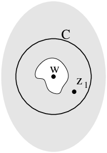
Proof. The initial observation is that, from CFT, correlation functions and are infinitely differentiable functions of (for non-colliding points lying in the domain of definition or ). Along with (4.2), this implies that is -differentiable. Note that by (4.2), we may in fact reduce the space of “inequivalent” correlation functions (i.e. that are not related by a product of functions of the individual positions) to a finite number of copies of open sets in and (the moduli space), so that -differentiability is essentially reduced to differentiability on a finite-dimensional manifold. Moreover, from (4.2) we clearly have
| (4.12) |
In particular, we have global stationarity, hence by Theorem 3.1 the global derivative exists. This proves A.
For the proof of B, first note that if contains , then vanishes as , so that we have the correct asymptotic condition. The proof then involves three steps: showing that and transform in agreement with (4.7), showing that they have the correct analytic structure for , and showing that for , they satisfy the correct boundary condition on . Then, by the discussion above, the equalities follow.
It will sometimes be convenient to consider the real and imaginary parts of separately; we will denote by the vector formed by these separated functions: .
The first step follows immediately from Theorem 3.2 in the case where . Otherwise, it uses Corollary 3.11 (which follows from Theorem 3.3) as follows. The invariance formula (4.12) implies that for any conformal on a domain , we have that , this being true on a -neighborhood of , and also that is -differentiable at . Moreover, the conditions of Theorem 3.3, with and as said, are clearly satisfied. These considerations in fact hold true for the real and imaginary parts of independently (i.e. hold for ). Replacing by (which we can of course do), we have
| (4.13) |
For simplicity, let us restrict to . Let us write for some , and consider conformal on . The right-hand side of (4.13) exists at and is continuous as for any fixed and . This is because the -neighborhood and -derivative of at exist for all , because represents, as a function of , a continuous path lying entirely in the moduli space for , and because we have infinite differentiability on the moduli space (and recall that the moduli space is a manifold). Hence we may take the limit on both sides. Similar arguments may be provided for other choices of , and we find that (4.13) holds for all conformal on . Hence, it holds for itself, in agreement with (4.7), which concludes the first step.
For the second step, we write , with and . The -differentiability and continuity conditions leading to (3.58) certainly hold at , hence we have, for instance in the holomorphic case,
Here, we may take to be any fixed point in . On the right-hand side, every term may have a pole of order up to 3 at (if ), but they cancel out since on the left-hand side there is no such singularity. Hence, we may simply omit these singularities. Here, it is convenient to simply subtract these singularities in each term on the right-hand side, hence to use the regularized holomorphic derivatives. That is, we have
| (4.14) |
For the first term, involving , note that we can extend the space of conformal maps acting on simply by omitting the requirement that they be conformal on . Then, we see that we have -differentiability as function of for any simply connected such that , so that the first term provides a holomorphic contribution to for . If , then obviously no -derivative needs to be taken, so the first term is 0. Hence, the singularities in may only come from the derivatives with respect to for . The conformal derivative formula (3.28) can be written, in the case of the first factor for instance, as
| (4.15) | |||||||
for any . From (3.45) and the form of the coefficient functions in (4.1), it is clear that only finite-order poles can occur, and, in , only at , in the function (except for the singularity at ). In order to establish exactly what these poles are, we only have to compare (4.15) with (4.3). Since in (4.15) we may evaluate the contour integrals by deforming them in , we see that the singularity of in is uniquely fixed by that of , and we conclude that it is the correct singularity for the stress-energy tensor. The singularity at the point , outside , is taken away in , without affecting other singularities. Since similar statements hold for anti-holomorphic counterparts, we find that and have the correct pole structure in . This concludes the second step.
For the third step, let us specialize to . We will show that
| (4.16) |
Since the right-hand side is holomorphic on , the left-hand side may be analytically extended to that region, and we may specialize to . There, by complex conjugation, we see that , hence putting together real and imaginary parts we obtain the correct boundary condition on .
In order to show (4.16), let us consider derivatives with respect to , and write, using (3.45),
where
Consider . We can find such that . Indeed, for any there is a unique conformal on such that , with, for instance, the normalization as . Consider , which is such that . For any fixed away from and , and have convergent Taylor expansions in about . It is easy to see that with we find . Hence, , so that we have
We then get
But since by (4.12), we obtain
The proof of Theorem 4.1 makes it clear that we can subdivide the action of the global derivative into its action on the various arguments of the correlation functions. In particular, if is the differential operator representing the pole structure of the holomorphic component of the stress-energy tensor,
with on
then we have on simply connected domains
where the regularized holomorphic derivative acts on in the way explained above (i.e. it acts on by conformal transformations). For instance, with primary fields, and re-writing the regularized holomorphic derivative as an integral, we have
| (4.17) |
In this form, it is apparent that the boundary of the domain of definition can be considered as a “continuum of zero-dimensional primary fields”, where can be interpreted as the holomorphic derivative with respect to the part of the boundary near .
4.4 One-point average
It is well known [38] that the one-point average of the stress-energy tensor on a domain can be expressed via a variation of the partition function on under a metric change, in a neighborhood of the flat, Euclidean metric (see (C.8)). This seems to point to an expression of the one-point average in terms of a conformal derivative. It turns out that the global holomorphic derivative used to reproduce the extended conformal Ward identities above can be used to reproduce as well the one-point average. However, the one-point average cannot simply be the global derivative of a partition function: the latter is not globally stationary in general. There is a particular ratio of partition functions, which we call relative partition function, that is globally stationary (in fact, globally invariant). This paticular ratio is inspired by results in the context of CLE [11], where a relative partition function is defined using CLE renormalized probability functions.
The relative partition function , depending on two domains and with , is defined as
| (4.18) |
(up to a constant factor). Our main formula in this subsection is that the one-point average can be expressed as
| (4.19) |
for (see figure 5).

The derivative is taken with respect to , where the action of conformal maps in a -neighborhood of is by conformal transformation of the set (the transformed set can then be interpreted as boundaries of two new simply connected domains and with ). In particular, the result of the derivative is independent of the domain . This means that, in general, correlation functions can be expressed as
where the derivative is with respect to (4.8) (which includes , with an action on in agreement with that above) and , and conformal maps act on as , with as in (4.10). By the transformation property (4.4), we see that the global derivative in (4.19) transforms in agreement with (3.55) and (3.56), where is the central charge. The derivation of (4.19) is reported in appendix C; it is based on CFT arguments, and is far from being of mathematical rigor55 5 This derivation appeared already in the preprint [11].. A more mathematically rigorous derivation for corresponding objects in the context of CLE is found in [11].
5 Conclusions
In the present paper, we have developed the notion of derivative on groupoids of conformal maps with (almost) a local manifold structure near to the identity. The main conclusion is that some fundamental aspects of CFT appear naturally in this general geometric context. More precisely, our first main result is that such a derivative, when there is global stationarity, can be described using an object with a clean analytic structure and simple transformation properties under conformal maps. Our second main result is that this object is, in fact, intimately related to the stress-energy tensor: it exactly reproduces the extended conformal Ward identities (the conformal Ward identities and the boundary conditions) for connected correlation functions. We also provided arguments indicating that it also reproduces the one-point averages of the stress-energy tensor.
Natural paths for extending and applying this work include: studying the full differentiable manifold of conformal maps (i.e. not just around the identity); extending to higher derivatives and stress-energy tensor descendants (a first part of which was done in [36]); generalizing to manifolds involving Lie groups so as to connect with other holomorphic symmetry currents in CFT; applying the formalism to deduce the form of the stress-energy tensor and other symmetry currents in other probabilistic theories connected to CFT (e.g. the Gaussian field); analyzing derivatives of functions characterizing other mathematical objects that may have close links with conformal maps; generalizing to a description of massive QFT.
Acknowledgments
I would like to thank D. Bernard and J. Cardy for asking questions in August 2008 that led to the present work, as well as C. Hagendorf, K. Kytola and, in particular, D. Meier for encouragements and helpful discussions. I also acknowledge support form an EPSRC First Grant, “From conformal loop ensembles to conformal field theorey” EP/H051619/1.
Appendix A Proof of structure of the continuous dual
We give an elementary proof of lemma 3.1.
Proof. Certainly, the set is part of the characterisation of . Consider . Then is given by (3.14) by linearity. But since in , we have by continuity. This shows (a).
If is a series of coefficients for some , , then so is any reassignment of signs of the s, because of absolute convergence of Taylor series in the disk of convergence. Hence, convergence of the r.h.s. of (3.14) implies that (3.18) is true (with ) for all . Suppose that we have a sequence of nonnegative reals such that the following is not true: . That is, suppose that . Let us construct the function , and the function that gives the smallest nonnegative integer such that for some . Since as , then the sequence of strictly increasing integers that takes as is an infinite sequence. We also consider the sequence of the doublets for all , with the corresponding values of such that . Let us construct the sequence with elements given by for , and otherwise. For any given , there is a such that ; moreover, as increases, this increases. Then, for any , we have that for all large enough. Hence, for some , because converges for any . On the other hand, the series diverges (is infinite) because for and otherwise, and is an infinite sequence. This shows that if (3.18) holds, then . As a consequence, any gives rise to a function in (3.15) that is holomorphic on . This shows (b).
Since then (3.17) gives rise to the correct action of on the basis, and gives rise to a continuous mapping, by (a) it is true that the class completely characterizes any . If two functions and are both in , then is holomorphic on , and if additionally both are holomorphic in , then is holomorphic on . Since , it must be that . Suppose the relation (3.17) holds for all , and both for and for . We can always isolate the holomorphic part by taking linear combinations of the cases with and with , so that by subtracting, we have for all . Since is holomorphic on an annulus with as part of its boundary, we can write (by Cauchy’s integral formula) where is holomorphic on , and is holomorphic on (i.e. in a neighborhood of this closed set). We are left with . Taking for , we show that all coefficients of the Taylor expansion of about are zero, hence that . Hence, , so that and are in the same class. A similar argument holds for . Thanks to (b), this shows (c), and then immediately implies (e).
Appendix B Factorisation of conformal maps on annular domains
In this appendix, we work out one result that is needed in the proof of Theorem 3.3. In order to make the derivation clearer, we will employ a simpler notation than what is used in that proof. Consider two simply connected domains and such that ; then is an annular domain of . If a conformal map on is near enough to the identity, then it can be factorized: we can write it as a composition of a map conformal on and a map conformal on . We express this result more precisely as follows (we will use the phrase winding annular subdomain of an annular domain to designate an annular subdomain that separates the boundary components ).
Theorem66
6
There is a more general theorem of factorization, not needing the smallness condition of ; a proof of this more general theorem using the uniformization theorem for Riemann surfaces can be found in [40], and earlier proofs in [39, 41]. But the present theorem is sufficient, and its present proof has some content which may be of interest besides the particular problem at hand.
I. Consider two simply connected domains and such that . For any compact subset that contains some winding annular subdomain of , there exists a such that any map conformal on satisfying:
- 1.
where is the distance in the round metric on the Riemann sphere,
- 2.
there are open neighborhoods of and of such that ,
is factorizable: there exist a map conformal on and univalent on , and a map conformal on , such that
| (B.1) |
on .
We may always simplify the problem by considering, instead of , the map for some fixed Möbius map . Hence, we may assume without loss of generality that (in fact we may take ). Likewise, we may consider, instead of , the map for some fixed Möbius map ; then we may assume without loss of generality that . We will assume these two properties. Further, we may replace the round-metric distance by the plane distance ; we will do this in the following.
Then, we can also modify the maps and without changing by writing with another Möbius map. Thanks to this, we can assume without loss generality that 1) if , then as , and 2) if , then and as (note that is contained in or , but not both, by our previous assumption).
II. By choosing , and as above, the following integral equations hold:
| (B.2) | |||||
| (B.3) |
The right-hand side of (B.2) should be understood as the analytic continuation of an expression with contour and argument in a subdomain of where is univalent.
Proof
We may consider and satisfying the assumptions above, and look for and such that the point 1 of part I holds.
Let us first prove that with an appropriate choice of , there must be a winding annular subdomain of where is univalent.
The minimal distance between and is finite and non-zero. Let us choose such that contains the closure of a winding annular subdomain with the minimal distance between the two components of being greater than . Then, with for , we now show that the map is univalent on the winding annular subdomain with at every point a distance from . Indeed, suppose it is not univalent there. Then consider such that and . Consider also a smooth, simple, unwinding curve from to . Then is a smooth loop a distance less than away from . The loop may have double or higher order points; if it does, we look at the pre-image of these points on and choose new and such that is a simple loop. Then, there must be parts of the boundary of on both simply connected components of . This is because is conformal in a neighborhood of the loop , hence can be analytically continued from there, and is doubly valued in a neighborhood of . Hence the analytic continuation in any simply connected component of must give rise to a branch point, which would map to a non-conformal point of . This has to be shielded by the boundary of , hence also by the boundary of . Since, then, there are parts of the boundary of on both simply connected components of , and since the loop is a distance less than from , hence more than from , this means that parts of the boundary are mapped further away than a distance , a contradiction with the condition for .
Suppose that we find a factorization on , where is univalent, instead of a factorization (B.1) on (with and simply connected domains, and ). Suppose also that is univalent on . Clearly, then, is univalent on the annular domain , hence on .
Then, we may extend the factorization to one that is valid on the whole by analytic continuation.
Indeed, the definition agrees with on , and extends analytically (but not necessarily univalently) to with , since , , and is conformal on . We will use the same symbol for the resulting analytic map extended to all of . The conformality conditions and for further guarantee that is in fact conformal on .
Hence we have a factorization on . The definition agrees with on , and we may try to extend it analytically (but not necessarily univalently) to . The two possible obstructions are if maps outside of , the domain of , or if the analytic continuation is multiply-valued because of the (possible) multiple-valuedness of . But is , hence the second condition in part I of the theorem guarantees to be in . Moreover, the analytic continuation will be unique, because two topologically different paths in between two given points must cross , and single-valuedness of on as well as the second condition of part I of the theorem forbids the image under of any path in to cross . We will use the same symbol to designate the resulting analytic map extended to all of . The conformality conditions and for further guarantee that is in fact conformal on .
Finally, on so that is univalent on as well, and so that . Then, we recover the factorization (B.1) (renaming ) for the full domain .
Hence, it is sufficient to assume to be univalent on . Moreover, by analytic continuation arguments as above, we may assume that both and are smooth, by replacing and by appropriate subdomains. Then, we are looking for a factorization (B.1) for conformal univalent on and conformal (and hence also univalent) on .
Let us write
| (B.4) |
Certainly, is holomorphic on . Suppose that for two conformal maps (univalent conformal on ) and (univalent conformal on ), the following equations hold:
| (B.5) | |||||
| (B.6) |
Then we have, for ,
Replacing the term by its expression (B.5), we find
where the second equation is obtained by Cauchy’s theorem. Hence, if the integral equation (B.5) has a univalent conformal solution on , and that the resulting from (B.6) is conformal on , we have found a factorization. This factorization has the properties required for part II of the theorem, hence this would also prove part II.
The integral equation for can be written for its inverse as follows (with ):
| (B.7) |
From there, it is obvious that is holomorphic on (with the correct behavior around ), and we only need to check that there and that is univalent on .
We now show that for “small enough” (as in the theorem), there is a solution giving and with the right properties.
The first part of the strategy is essentially to show that the process of solving the integral equation (B.7) recursively, starting with , converges to a holomorphic function. Let us write
with and
| (B.8) |
for some simply connected domain (different from the in the first part of the proof). Clearly, is holomorphic for in a neighborhood of , if for . Let us denote by the supremum of for . Let us choose as well as another simply connected domain in such a way that is a non-empty winding annular subdomain of , and that the smallest distance between and is the same as the smallest distance between and . Let us also choose a number , and denote . Then, if we indeed find for . We will show by induction that for small enough on , the condition for all implies , which shows that is holomorphic on a neighborhood of for all .
Let us then assume that for all , and consider the differences . They satisfy
We now bound the integral involved. For a function holomorphic on , where has a finite supremum denoted by , we can always bound the absolute value of the integral by for , where is the length of and is the distance from to (we imagine taking an integration path along ). For , we can move the integration path away from before bounding the absolute value, and we can always keep it far enough by bringing it through if necessary and taking the residue at . More precisely, take to be the curve at all points equidistant to and . Consider the components and of , the first containing the domain . For , we could still take the integration path to be ; for , we could take the integration path to be . In the first case, the bound is still ; in the second case, it is with the length of and the distance from to . We can define the function by absorbing all factors:
Then, we have
Note that is an increasing function for going away from , and that it has an infimum on that is greater than 0, i.e.
where is the smallest distance between and .
In our case, we have . We write this as
We can take the contour to be the oriented boundary of the winding annular subdomain of which is such that is at each point a distance from . Then, for , we can bound the absolute value of the contour integral by where is the length of , and is the supremum of on . Hence, we have
where . Then, we find, for ,
where is the supremum of for . Since increases as goes away from , the number is also the supremum of for . Solving for this supremum (because by assumption, the bound holds for smaller as well), this gives
For small enough so that
| (B.9) |
we can now bound :
and since , we have, using the previous method and ,
where is the supremum of on . Hence, we find the bound
Then, for
| (B.10) |
we indeed find that , which completes the induction. Note that given the domains and the number , the quantities , and are fixed, as well as the domain determining where the supremum of is taken. Condition (B.10) can be solved for , giving
| (B.11) |
Hence, this condition is stronger than (B.9), so is sufficient.
Now we can show that with (B.11) (in fact, only (B.9) is required), converge uniformly as on , implying that there is a holomorphic solution to (B.7) with replaced by . Indeed, we have that the sequence converges uniformly and exponentially to 0 for . Hence, the series also converges uniformly for (because the remainder of the partial sum satisfies as uniformly for ). Hence, the limit of the sequence of holomorphic functions is a function that is holomorphic on , and bounded on by
| (B.12) |
The limit can be taken on both sides of (B.8), and uniform convergence gives the result.
Let us now consider the function
| (B.13) |
which solves (B.7) (with replaced by ). This function is not only holomorphic, but also conformal on for all small enough (possibly smaller than the bound (B.11)). Indeed, we can bound the absolute value of by bounding
using similar techniques as those above, and using (B.12); this guarantees that for small enough, .
Note that in (B.13) compactly tends to the identity as . Hence, for all small enough, there is a domain inside where is univalent conformal, and this domain tends to as . Then, inverting, we have found a solution to (B.5), where is replaced by . The function is univalent conformal on , and by the construction above, we know that . For , we have that . Hence, by taking small enough, we can guarantee that . Then, we can construct by (B.6). The function is analytic on . The domain tends to as , so that the function converges compactly to the identity on . Hence, for small enough, is univalent conformal on a domain . Again by choosing small enough, we can guarantee that the domain has its boundary inside , i.e. , since as and . That is, we have found a factorization (B.1) on , a winding annular subdomain of .
By the analytic continuation argument already stated above, and using the fact that is univalent on (by our simplifying assumption), we get a factorization on .
Hence, we have found a factorization on , with univalent conformal on and univalent conformal on . Note that we can always choose and small enough so that is close enough to in order for to be inside the compact set . With our previous arguments to extend to the non-univalent case, this completes the proof.
Appendix C Derivation of the one-point average formula
First, we need to describe how a conformal transformation of the domain of definition of a partition function is connected to a change of metric.
A conformal transformation of the domain of definition can be seen as a result of two steps: a re-parametrization of the initial domain, which obviously keeps the partition function invariant but changes the metric by an overall space-dependent factor, and a Weyl transformation that brings back the original metric, but under which the partition function transforms [42]. We use the standard setup where the trace of the bulk stress-energy tensor is zero, hence the metric we use is flat in the bulk (there is no trace anomaly, see for instance [3]) – it can be taken as the Euclidean metric. Then, we consider a partition function on with that metric, and in the first step, we use as a parameter space for the domain . The metric it gives on (in the bulk) is obtained by . In the second step, the Weyl transformation with a factor brings the metric back to the Euclidean metric on , and we have a partition function on .
The transformation of the CFT partition function under a Weyl transformation was found by Polyakov in the context of random surfaces [42]: for any appropriate domain (say, any domain with piecewise smooth boundary), we have
| (C.1) |
where is the CFT central charge and is the Liouville action of on ,
| (C.2) |
Here, is the metric on (and is its determinant), is the associated scalar curvature and is some UV-divergent, non-universal (i.e. lattice-model-dependent) scale. Our choice for is the Kronecker delta in the bulk of .
In general, with curved boundaries, the curvature must have a non-zero contribution supported on the boundary. It is important that the integral in the Liouville action (C.2) covers the boundary of (which is the meaning of the notation ), so that it gets a non-zero contribution from this term. We will not need a precise description of the boundary term of the metric, but only some properties of the resulting contribution to the Liouville action. We will need that the contribution of the boundary to the Liouville action only depends on the linear curvature along (besides the value of the function on ). We will denote this contribution by , where is the oriented boundary of , counter-clockwise around the interior of .
Clearly, the partition function in general is not invariant under global conformal maps. Hence, we cannot define the global derivative on it. However, it turns out that there is a certain ratio of partition functions, which we call the relative partition function, that is globally invariant. This particular ratio was inspired by results in the context of CLE [11]. The relative partition function , depending on two domains and with , is defined as
| (C.3) |
up to a constant factor. Let us consider a map that is conformal on and maps it to a domain of . Then, there is also a map conformal on such that . Similarly to the case of correlation functions, we see as a function of and , keeping on the component of . Let us consider the ratio
| (C.4) |
We will argue that this ratio is in fact independent of , unity for a global conformal transformation, and, in some sense, universal. We will then provide further CFT arguments to show, from this formula, that the global derivative reproduces the stress-energy tensor one-point average.
First, using the transformation property (C.1), we find
| (C.5) | |||||
Note the careful inclusion/exclusion of domain boundaries in the Liouville actions. The last expression clearly is independent of . Also, suppose is a global conformal transformation. Then we can choose so that , and we are left with (there is no boundary contribution). This is independent of ; that it should be 1 can then be obtained simply by sending and (assuming continuity). In order to argue that the right-hand side of (C.5) is universal in some way, we need to argue that it is mostly independent of (the parameter in the Liouville action (C.2)). Since , the -terms in can be combined into an integration over by change of coordinates; this then provides an overall factor that is independent of . This factor is seen to be 1 by setting (that is, ). As for the expression , there is a non-trivial metric on , which we did not specify; but we expect that the resulting combination of -terms is universal.
Second, we want to evaluate the derivative of and show that it is the stress-energy tensor. Since this is the first derivative, the terms that are quadratic in in the Liouville actions do not contribute. Also, as we argued above the bulk -terms cancel out, and the bulk curvature terms are zero since the bulk metric is flat77 7 There is a subtlety with the point at when the domain contains it: it takes all the curvature of the Riemann sphere. However, a careful calculation with the metric , where the curvature is re-distributed, shows that the limit of the curvature term of the Liouville action gives zero contribution to the first derivative.. This means that we are left only with the boundary contributions to the Liouville actions. Hence we find:
| (C.6) |
Note that with an appropriate renormalization of the partition function , we could guarantee that (that is, the boundary contributions simply get a minus sign for an opposite linear curvature of the boundary). Then, we would obtain
| (C.7) |
On the right-hand side, we have not a single partition function, but a product. Again, this product guarantees that the derivative in directions of small global conformal transformations is zero. Yet, there is no ambiguity as to “where” the stress-energy tensor is inserted: the point must lie in , and the analytic continuation of the function of that is obtained does not reproduce the derivative at points outside .
But let us come back to (C.6). Evaluating it directly would need a more precise understanding of the boundary terms in the Liouville actions. However, there is way of relating these boundary contributions to the stress-energy tensor without an explicit evaluation. Indeed, the stress-energy tensor may in fact be defined as the field generating the variation of the partition function under a change of metric [38]:
| (C.8) |
Here, is some domain, and is the symmetric stress-energy tensor in the canonical normalization (in this normalization, the charge , in the quantization on the line, generates -derivatives with coefficient 1). With tracelessness , it is related to the holomorphic and anti-holomorphic components and via
| (C.9) |
This involves both a “change of coordinates” , as well as a change of normalization in order to guarantee the correct CFT normalization of and .
Under a transformation that is conformal on the domain of definition, with small, the metric changes diagonally, , so that we obtain the one-point function of the trace of the stress-energy tensor in (C.8). This trace is zero except at the boundary, hence we are left with a boundary integration, as expected by the previous considerations. If we take for some small complex , we can evaluate by extracting the part proportional to in , and discarding the part proportional to , as long as . If , we have to find a function that has the same infinitesimal effect on but that is holomorphic on . In this way, we could evaluate both terms on the right-hand side of (C.6): the first term by evaluating under , the second by evaluating under and discarding the part that is integrated along .
Finding in general is complicated. The simplest way to evaluate under is rather to evaluate under and take the limit where – we just make a puncture at . Evaluating the contribution of the puncture can be done via (C.8), where the bulk metric change is singular at , and not diagonal there. Denoting this contribution by , we simply find that
and hence that
| (C.10) |
This formula quite directly leads to the one-point function of the stress-energy tensor (see below). In terms of the expression (C.7), these considerations suggest that the product takes care of the boundary conditions, upon inserting the bulk stress-energy tensor, by a “method of images.” Also, we see that the presence of the domain in the relative partition function has the important effect of cancelling the boundary contributions to the singular metric change, so that only the puncture contribution remains.
References
- [1] A.A. Belavin, A.M. Polyakov and A.B. Zamolodchikov, Infinite conformal symmetry in two-dimensional quantum field theory. Nucl. Phys. B 241 (1984) 333.
- [2] P. Ginsparg, Applied conformal field theory, in: Les Houches, session XLIX (1988), Champs, cordes et phénomènes critiques / Fields, strings and critical phenomena, Eds. E. Brézin and J. Zinn-Justin, Elsevier, New York (1989).
- [3] P. Di Francesco, P. Mathieu and D. Senechal, Conformal Field Theory, Berlin, Springer (1997)
- [4] J. Lepowsky and H. Li, Introduction to Vertex Operator Algebras and Their Representations, Progress in Mathematics, Vol. 227, Boston, Birkhäuser, 2004
- [5] D. Friedan, S. Shenker, The analytic geometry of two-dimensional conformal field theory, Nucl. Phys. B 281 (1987) 509.
- [6] J. Cardy, SLE for theoretical physicists, Ann. Phys. 318 (2005) 81.
- [7] S. Sheffield, Exploration trees and conformal loop ensembles, Duke Math. J. 147 (2009) 79.
- [8] S. Sheffield and W. Werner, Conformal loop ensembles. The Markovian characterization, arXiv:1006.2374.
- [9] S. Sheffield and W. Werner, Conformal loop ensembles, Construction via loop-soups, arXiv:1006.2373.
- [10] B. Doyon, V. Riva and J. Cardy, Identification of the stress-energy tensor through conformal restriction in SLE and related processes, Comm. Math. Phys. 268, 687 (2006)
- [11] B. Doyon, Conformal loop ensembles and the stress-energy tensor, I. Fundamental notions of CLE. arXiv:0903.0372; II. Construction of the stress-energy tensor. arXiv:0908.1511 (2009).
- [12] R. Friedrich, The global geometry of stochastic Loewner evolutions, arXiv:0906.5328, Conference Proceedings, The first MSJ-SI, Probabilistic Approach to Geometry (2008).
- [13] J. Cardy, Conformal Invariance and Surface Critical Behavior, Nucl. Phys. B 240, 514 (1984)
- [14] A. A. Kirillov, A Kähler structure on K-orbits of the group of diffeomorphisms of the circle, Funct. Anal. Appl. 21 (1987) 122.
- [15] A. A. Kirillov and D. V. Yur’ev, Kähler geometry of the infinite-dimensional homogeneous space , Funct. Anal. Appl. 21 (1987) 284.
- [16] O. Lehto, Univalent Functions and Teichmuller Spaces, Springer-Verlag, New York Berlin Heidelberg, 1986.
- [17] S. Nag and A. Verjovsky, and the Teichmüller spaces, Commun. Math. Phys. 130 (1990) 123.
- [18] M.J. Bowick and S.G. Rajeev, The holomorphic geometry of closed bosonic string theory and , Nucl. Phys. B 293 (1987) 348
- [19] B. Zumino, The geometry of the Virasoro group for physicists, in the NATO Advanced Studies Institute Summer School on Particle Physics, Cargèse, France, 1987.
- [20] S. Nag, On the tangent space to the universal Teichmüller space, Ann. Acad. Scient. Fennicae 18 (1993) 377.
- [21] M. Gordina and P. Lescot, Riemannian geometry of , J. Func. Anal. 239 (2006) 611
- [22] R. Friedrich and J. Kalkkinen, On conformal field theory and stochastic Loewner evolution, Nucl. Phys. B 687 (2004) 279.
- [23] R. Friedrich, A renormalization group approach to stochastic Loewner evolutions, in: Combinatorics and physics, Eds. K. Ebrahimi-Fard, M. Marcolli, W. D. ven Suijlekom, Cont. Mathematics, vol. 539, AMS publications, Providence, Rhode Islands, 89-114, 2011.
- [24] W. Taylor IV, Coadjoint orbits and conformal field theory, Ph.D. thesis, University of California at Berkeley (1993), hep-th/9310040.
- [25] V. Arnold, Sur la géométrie différientielle des groupes de Lie de dimension infinie et ses applications à l’hydrodynamique des fluides parfaits, Ann. Inst. Fourier 15 (1966) 319.
- [26] R. Hamilton, The inverse function theorem of Nash and Moser, Bull. Amer. Math. Soc. 7 (1982) 66.
- [27] J. Milnor, Remarks on infinite-dimensional Lie groups. In Relativity, groups and topology, II (Les Houches, 1983), pages 1007Ð1057. North-Holland, Amsterdam, 1984.
- [28] A. A. Kirillov, Geometric Approach to Discrete Series of Unireps for Vir, J. Math. Pures Appl. 77 (1998) 735.
- [29] Yu. A. Neretin, A complex semigroup that contains the group of diffeomorphisms of the circle, Funct. Anal. Appl. 21 (1987) 160.
- [30] M. Bauer and D. Bernard, Conformal transformations and the SLE partition function martingale, Ann. Henri Poincaré 5 (2004) 289.
- [31] A. Weinstein, Groupoids: unifying internal and external symmetries, Notices Amer. Math. Soc. 43 (1996), 744.
- [32] A Kriegl and W. Michor, The Convenient Setting of Global Analysis, Mathematical Surveys and Monographs, 53, AMS Publications, Providence, Rhode Islands, 1997.
- [33] V. C. Varadarajan, Lie Groups, Lie Algebras and their Representations, 2nd edition, Prentice-Hall series in modern analysis, Prentice-Hall, Englewood Cliffs, New Jersey, 1984.
- [34] W. Rudin, Functional analysis, New-York, McGraw-Hill (1973)
- [35] V.I. Averbuh and I.G. Smolyanov, The theory of differentiation in linear topological spaces, Russ. Math. Surv. 22, 201 (1967); The various definitions of the derivative in linear topological spaces, Russ. Math. Surv. 23, 67 (1968)
- [36] B. Doyon, Higher conformal variations and the Virasoro vertex operator algebra, arXiv:1110.1507.
- [37] J.B. Conway, A course in functional analysis, New-York, Springer-Verlag (1990)
- [38] D. Friedan, Introduction to Polyakov’s string theory, in: Les Houches, session XXXIX (1982), Développements récents en théorie des champs et mécanique statistique / Recent advances in field theory and statistical mechanics, Eds. J.-B. Zuber and R. Stora, Elsevier, New York (1984)
- [39] O. Hübner, Die Faktorisierung konformer Abbildungen und Anwendungen, Math. Zeitschr. 92 (1966) 95.
- [40] B. Doyon, Factorization of conformal maps on finitely connected domains, arXiv:1107.0582.
- [41] R. Kühnau, Einige elementare Bemerkungen zur Theorie der konformen und quasikonformen Abbildungen, Math. Nach. 45 (1970) 307.
- [42] A. M. Polyakov, Quantum geometry of bosonic strings, Phys. Lett. B 103, 207 (1981)