An environmental Butcher-Oemler effect in intermediate redshift X-ray clustersThanks: Based on observations obtained with MegaPrime/MegaCam, a joint project of CFHT and CEA/DAPNIA, at the Canada-France-Hawaii Telescope (CFHT) which is operated by the National Research Council (NRC) of Canada, the Institut National des Science de l’Univers of the Centre National de la Recherche Scientifique (CNRS) of France, and the University of Hawaii. This work is based in part on data products produced at TERAPIX and the Canadian Astronomy Data Centre as part of the Canada-France-Hawaii Telescope Legacy Survey, a collaborative project of NRC and CNRS.
Abstract
We present uniform CFHT Megacam and photometry for 34 X-ray selected galaxy clusters drawn from the X-ray Multi-Mirror (XMM) Large Scale Structure (LSS) survey and the Canadian Cluster Comparison Project (CCCP). The clusters possess well determined X-ray temperatures spanning the range . In addition, the clusters occupy a relatively narrow redshift interval () in order to minimize any redshift dependent photometric effects. We investigate the colour bimodality of the cluster galaxy populations and compute blue fractions using criteria derived from Butcher and Oemler (1984). We identify a trend to observe increasing blue fraction versus redshift in common with numerous previous studies of cluster galaxy populations. However, in addition we identify an environmental dependence of cluster blue fraction in that cool (low mass) clusters display higher blue fractions than hotter (higher mass) clusters. Finally, we tentatively identify a small excess population of extremely blue galaxies in the coolest X-ray clusters (essentially massive groups) and note that these may be the signature of actively star bursting galaxies driven by galaxy-galaxy interactions in the group environment.
1 Galaxy populations in clusters
The observed properties of galaxy populations reflect the environment in which they are located. Comparisons of galaxy populations drawn from low (the field) and high density (rich galaxy clusters) environments indicate that the population distribution described using measures such as current star formation rate (e.g. Balogh et al. 1999, Poggianti et al. 2006), integrated colour (e.g. Blanton et al. 2005) and morphology (e.g. Dressler et al. 1997, Treu et al. 2003) varies as a function of changing environment. From studies such as these it is clear that galaxies located in the cores of rich clusters display lower star formation rates, redder colours and more bulge dominated morphologies compared to galaxies located in the field.
Studies of the fraction of blue galaxies contributing to a galaxy cluster provided some of the first direct evidence for the physical transformation of galaxies in cluster environments. Butcher & Oemler (1984) reported an increase in the fraction of blue galaxies in 33 rich galaxy clusters out to compared to local clusters. However, subsequent studies designed to expand upon this initial discovery highlighted the many complexities associated with this relatively straightforward technique, including varying intrinsic cluster properties with redshift (e.g. X-ray luminosity as discussed by Andreon & Ettori 1999), the use of -corrections to determine rest frame colour distributions (Andreon, 2005) and the challenge of obtaining large samples with uniform photometry (successfully overcome by Loh et al. 2008).
In addition to the Butcher-Oemler (BO) effect measured employing optical galaxy colours, analogous BO-type effects have been reported as either a morphological BO effect (increasing spiral fraction in clusters with increasing redshift; Poggianti et al. 1999) and an infra-red (IR) BO effect (increasing fraction of dust enshrouded star forming falaxies in clusters with increasing redshift; Duc et al. 2002; Saintonge et al. 2008) to name two examples.
An alternative approach is to consider an environmental Butcher-Oemler effect whereby one attempts to determine the variation of blue fraction as a function of varying intrinsic cluster properties selected over narrow redshift intervals. This has been achieved by comparing blue fractions within clusters at increasing clustercentric radii (e.g. Ellingson et al. 2001; Loh et al. 2008) or by considering blue fractions measured between clusters of differing X-ray luminosities (e.g. Wake et al. 2005). A number of studies report the decrease of the fraction of blue galaxies with decreasing scaled clustercentric radius, e.g. the virial radius determined employing either cluster dynamics (Ellingson et al., 2001), correlation properties (Loh et al., 2008), or extrapolated from X-ray properties (Wake et al., 2005).
The currently favoured explanation for these observed trends is that infalling field galaxies are processed physically as they travel from the field, through the cluster outskirts and virialise in the central cluster region (Berrier et al., 2009). However, the extent to which cluster galaxies were ‘‘pre-processed’’ by physical effects occuring during an earlier residence in a galaxy group11 1 Note that we generally refer both groups and clusters of galaxies as ”clusters” in this paper and quantify our description using the X-ray temperature. remains contested (Li et al., 2009). Numerous physical processes have been suggested as the agents of this apparent transformation of galaxy populations. However, the dominant physical process(es) to which an infalling galaxy is subject remains unclear.
The two principal examples of such processes are ram pressure stripping and galaxy galaxy interactions. Ram pressure stripping describes the effective force experienced by the diffuse gas component of the infalling galaxy as it travels through the hot, dense intra-cluster medium (ICM; Gunn & Gott 1972). Both hot and cold gas may be stripped from the infalling galaxy leading to the exhaustion of the available gas supply that will otherwise cool and form stars (Abadi et al. 1999; Kawata & Mulchaey 2008; McCarthy et al. 2008). Hydrodynamical simulations have indicated that the ICM associated with galaxy group and cluster environments will strip of order 70% to 100% respectively of hot gas from a typical infalling spiral galaxy within one crossing time (Kawata & Mulchaey 2008; McCarthy et al. 2008). The effect is manifest as a sharp decline in the galaxy star formation rate effective on a timescale comparable to the rate at which the unstripped cold gas supply is consumed. The observations of a population of red (i.e. passive) spiral galaxies contributing to the red sequence would appear to support the view that some fraction of galaxies experience the stripping of disc gas via ram pressure effects (Wolf et al., 2009). The observation of galaxies displaying extended HI tails in the Virgo cluster (Chung et al., 2007) is nominally consistent with the expectations of ram pressure stripping. However, we note that the authors also report the presence of close companions to these galaxies in a number of cases and comment that a combination of ram pressure and tidal stripping provides a more compelling explanation.
When referring to galaxy-galaxy interactions we note that this may indicate one of a wide range of encounters. Interactions may be predominantly tidal between close neighbours resulting in halo gas being moved outward where it is more readily stripped (e.g. Chung et al. 2007). High speed encounters (either referred to as harrassment or threshing in the literature) may also result in tidal stripping of halo gas (Moore et al., 1996). Finally, infalling galaxies may merge with existing cluster members. The products of such merger encounters may be predicted by considering the mass ratio of the merging galaxies: large mass ratios result in enhanced star formation in the satellite galaxy yet may not lead to a star burst in the more massive companion (Cox et al., 2008). Equal mass mergers on the other hand result in the complete disruption of the infalling spiral galaxy (for example) to form a bulge dominated system accompanied by a significant central star burst (Di Matteo et al., 2007). The internal disruption associated with such strong interactions can result in a short term enhancement in star formation followed by a rapid exhaustion of the available cold gas supply. The potential effect of such strong galaxy-galaxy interactions is of interest to studies of the environmental dependence of galaxy evolution as the merging rate (the product of relative velocity and interaction cross section) is predicted to be a strong function of environment: the cross section for disruptive encounters increases as the cluster velocity dispersion approaches the internal velocity of the infalling galaxy (Makino & Hut, 1997). Compelling evidence for enhanced galaxy-galaxy interactions in rich cluster environments is provided by Hubble Space Telescope (HST) observations indicating a high merger fraction in such environments compared to field comparison samples (Dressler et al. 1994; van Dokkum et al. 1999). However, such observations must be contrasted with mid-infrared selected moderate starburst galaxies located in rich cluster environments whose optical morphologies resemble undisturbed spiral galaxies (Geach et al. 2009; Oemler et al. 2009).
A picture is therefore emerging whereby multiple mechanisms (ICM stripping, merger induced star formation and tidally induced star formation) may participate in the physical processing of infalling galaxies. Currently unanswered questions focus upon whether more than one physical process acts upon a typical galaxy falling into a dense environment (and which might be considered dominant) and whether the relative importance of each of the suggested physical processes changes as a function of the global properties of the group/cluster environment into which the galaxy falls. In this paper we attempt to answer the related question of whether the effectiveness of galaxy processing can be determined as a function of global cluster environment. Our approach is to compute the blue fraction as defined by Butcher & Oemler (1984) for a sample of X-ray selected galaxy clusters and to determine whether the blue fraction displays a significant trend versus X-ray temperature (here employed as a proxy for the global cluster mass).
Throughout this paper, values of , and are adopted for the present epoch cosmological parameters describing the evolution of a model Friedmann-Robertson-Walker universe. All magnitude information is quoted using AB zero point values.
2 The galaxy cluster sample
The data presented in this paper are drawn from two complementary samples of X-ray selected galaxy clusters. Clusters with X-ray temperatures keV are drawn from the X-ray Multi-Mirror (XMM) Large Scale Structure (LSS) survey. Clusters are selected from the 5 deg2 “Class 1” sample of Pacaud et al. (2007) according to X-ray temperature keV and spectroscopic redshift (Figure 1). Such relatively cool X-ray clusters are often referred to as galaxy groups in the literature. However, all X-ray selected systems considered in this paper are referred to as “clusters” for simplicity. The above criteria generate a sample of 11 clusters which are referred to as “cool” in the following analysis.

Clusters with X-ray temperatures keV are selected from the sample of Horner (2001) and form part of the Canadian Cluster Comparison Project (CCCP; Bildfell et al. 2008). Although the final CCCP sample will contain some 50 X-ray selected galaxy clusters, we consider here the 27 systems with accompanying optical data obtained using the Canada France Hawaii Telescope (CFHT) MegaCam imager (see below). Due to the large temperature range covered by the CCCP sample () we further subdivide the CCCP sample into “mid” clusters displaying and “hot” displaying keV. We limit the CCCP sample to redshifts in order to maximise the available sample size while reducing the redshift interval over which photometric quantities are -corrected to a common epoch. These considerations limit the size of the mid and hot samples to 18 and 5 clusters respectively. The X-ray properties of all clusters are shown in Table 1.
The CCCP clusters all lie above the nominal X-ray flux limit of the XMM-LSS survey and cover the full range of scatter observed in scaling relations such as the X-ray relation. In this sense, the CCCP clusters would all be detected by X-ray images of the same quality as the XMM-LSS survey images (irrespective of how the CCCP cluster were originally selected). However, XMM-LSS lacks the areal coverage to detect such massive clusters which display low sky surface densities. Therefore, the combined XMM-LSS/CCCP sample is a representative, (largely) unbiased sample of X-ray clusters with temperatures . We note that the XMM LSS clusters populating the cool sample are moderately biased toward higher X-ray luminosities than the average cluster population at that temperature (see Pacaud et al. 2007 Figure 8). This implies a moderate bias toward gas rich or centrally condensed systems which we will recall at relevent points in the following discussion.
The characteristic cluster scaling radii employed in this work are based upon . This is defined as the radius at which the enclosed cluster mass density equals 500 times the critical density of the universe at the cluster redshift (Pacaud et al., 2007). Converting the relation of Finoguenov et al. (2001) to a CDM cosmology, Willis et al. (2005) define
| (1) |
where T measured X-ray temperature in keV and is the Hubble constant in units of .
| Cluster | R.A. | Dec. | z | ||
| (deg.) | (deg.) | (keV) | (kpc) | ||
| XLSSC 13 | 36.858 | -4.538 | 0.31 | 340 | |
| XLSSC 51 | 36.498 | -2.826 | 0.28 | 384 | |
| XLSSC 44 | 36.141 | -4.234 | 0.26 | 399 | |
| XLSSC 08 | 36.337 | -3.801 | 0.30 | 387 | |
| XLSSC 40 | 35.523 | -4.546 | 0.32 | 402 | |
| XLSSC 23 | 35.189 | -3.433 | 0.33 | 497 | |
| XLSSC 22 | 36.916 | -4.857 | 0.29 | 472 | |
| XLSSC 25 | 36.353 | -4.679 | 0.26 | 533 | |
| XLSSC 18 | 36.008 | -5.090 | 0.32 | 615 | |
| XLSSC 27 | 37.014 | -4.851 | 0.29 | 653 | |
| XLSSC 10 | 36.843 | -3.362 | 0.34 | 574 | |
| MS0440+02 | 70.805 | 2.166 | 0.19 | 957 | |
| A1942 | 219.600 | 3.669 | 0.22 | 957 | |
| A0223 | 24.477 | -12.815 | 0.21 | 964 | |
| A2259 | 260.033 | 27.668 | 0.16 | 1007 | |
| A1246 | 170.9972 | 21.482 | 0.19 | 1078 | |
| A2537 | 347.092 | -2.187 | 0.30 | 1039 | |
| A0959 | 154.433 | 59.556 | 0.29 | 1022 | |
| A0586 | 113.072 | 31.637 | 0.17 | 1127 | |
| A0115 | 13.980 | 26.422 | 0.20 | 1120 | |
| A0611 | 120.228 | 36.065 | 0.29 | 1100 | |
| A0521 | 73.510 | -10.244 | 0.25 | 1106 | |
| A2261 | 260.609 | 32.139 | 0.22 | 1153 | |
| A2204 | 248.192 | 5.574 | 0.15 | 1247 | |
| MS1008-12 | 152.632 | -12.652 | 0.30 | 1169 | |
| CL1938+54 | 294.555 | 54.159 | 0.26 | 1200 | |
| A0520 | 73.554 | 2.924 | 0.20 | 1262 | |
| A1758 | 203.205 | 50.538 | 0.28 | 1186 | |
| A2111 | 234.914 | 34.429 | 0.23 | 1267 | |
| A0851 | 145.746 | 46.9945 | 0.41 | 1291 | |
| A0697 | 130.740 | 36.3662 | 0.28 | 1343 | |
| A2104 | 235.029 | -3.3017 | 0.16 | 1438 | |
| A1914 | 216.512 | 37.8244 | 0.17 | 1444 | |
| A2163 | 243.920 | -6.1438 | 0.20 | 1663 |
2.1 Optical photometry
Optical photometry for the XMM-LSS and CCCP cluster samples is computed from CFHT Megacam images available for all fields. XMM-LSS clusters lie within the CFHT Legacy Survey (CFHTLS) wide synoptic survey22 2 http://www.cfht.hawaii.edu/Science/CFHTLS/ W1 area. The survey data consists of images taken in the CFHT filter set. Approximately 4 deg2 of the XMM-LSS footprint lies beyond the northern declination limit of the CFHTLS W1, of which 3 deg2 has been imaged as part of the XMM-LSS follow-up campaign using CFHT Megacam in the bands. Image exposure times in these additional fields are matched to the CFHTLS wide exposure times for each filter. The CCCP clusters considered in this sample were observed using CFHT Megacam as part of an optical follow-up of X-ray selected galaxy clusters (e.g. Bildfell et al. 2008). The processing of the CFHTLS wide data plus the northern extension and of the CCCP Megacam data are described in Hoekstra et al. (2006) and Bildfell et al. (2008) respectively. Image data is available in the and bands. Table 2 describes the main characteristics of each data set with Figure 2 showing -band number counts for the CCCP and W1 data compared with the CFHT Deep survey. We adopt a magnitude limit in all subsequent analyses in order that photometric samples drawn from all three data sets can be reasonably considered to be complete. Given the overlap in the photometric filters employed by XMM-LSS and CCCP we consider the photometric properties of cluster galaxies in the combined sample as determined using and bands.
| Sample | -band | -band | |
|---|---|---|---|
| (s) | (s) | seeing (″) | |
| XMM-LSS | 2500 | 2000 | 0.8 |
| CCCP | 1800 | 4800 | 0.7 |
Source extraction and photometry were performed using SExtractor v2.5.0 (Bertin & Arnouts 1996). Image regions affected by saturated stars and detector artefacts were excluded. Zero point information for sources detected in the CFHTLS W1 area plus northern extension was extrapolated from common sources detected in the Sloan Digital Sky Survey equatorial patch which overlaps the southern edge of the W1 area. Source photometry is quoted in AB magnitudes measured within 3″ diameter circular apertures.
Star-galaxy separation was performed by considering the -band half-light radius (HLR) versus -band magnitude distribution for sources in each Megacam field (Figure 3). The properties of instrument point spread function (PSF) that determines the half-light radius of the stellar locus varies systematically over the Megacam field. Considered over the entire field, this variation broadens the stellar locus and reduces the effectiveness of a single HLR cut at excluding stellar sources. The field itself is mapped onto a array of CCD detectors. We therefore determined the weighted mean HLR of the stellar locus in each Megacam CCD and rescaled the HLR values of all sources in each CCD such that the stellar values mapped on to a single locus defined in a reference CCD close to the optical centre of the detector. This operation reduced the effective dispersion of sources defining the stellar locus in each field (Figure 3) and permitted the application of a single threshold to exclude stellar sources33 3 We note that a component of the PSF variation over the Megacam field is anisotropic. However, for the purpose of star-galaxy separation, application of an isotropic scaling factor is sufficient..


3 Colour Magnitude Diagrams
Colour magnitude diagrams for each of the hot, mid and cool cluster samples are displayed in Figures 5, 6 and 7 respectively. All sources lie within of the measured X-ray centre of each cluster.
Computation of the blue fraction in each cluster first requires the red sequence relation defining the linear colour sequence followed by cluster early-type galaxies to be determined. This provides a reference value relative to which the blue galaxy population in each cluster may be defined. To determine the location of the red sequence we first applied a statistical background subtraction procedure to each cluster to highlight the population of cluster members. We applied the method of Pimbblet et al. (2002) whereby the field population and the cluster plus field population were each represented on a colour-magnitude grid. The probability that a galaxy occupying a particular grid position is field galaxy is then
| (2) |
were is an areal scaling factor used to match the area of the field sample to the cluster area. The field colur magnitude distribution is computed employing all galaxy sources at radii from the X-ray cluster centre. For each galaxy within of the cluster centre, membership was determined by comparing a random number in the interval [0,1] to the field probability value. This procedure was repeated 100 times for each cluster.
For each realisation, the red sequence location was computed employing a weighted, linear least squares fit and the mean slope and zero-point was calculated from the distribution of 100 values. To check and, if necessary, refine the location of the mean red sequence for each cluster we considered the “red edge” diagram for each system (an example of which is displayed in Figure 4). The red edge diagram shows the number of galaxies located at a colour offset at fixed -magnitude from the red sequence in a particular cluster. The zero-point of the red sequence was then adjusted to set the peak in the red edge distribution at zero colour offset.

This procedure worked well for the mid and hot cluster samples. However, following statistical background subtraction, the cool clusters typically possess insufficient cluster members to generate a reliable red sequence fit. In this case the red sequence relation computed for the stacked mid cluster sample described in Section 5 was applied to the cool clusters. The red sequence zero-point was adjusted using the red edge diagram procedure to provide an improved fit to individual clusters.
Figure 8 indicates the colour of the red sequence measured at fixed absolute magnitude () versus redshift for the mid and hot clusters. The colour uncertainty is computed as the standard deviation of the red sequence zero-points as measured for the 100 realisations of the cluster subtraction procedure. The -correction employed to convert absolute -magnitude to apparent -magnitude at the redshift of each cluster assumes a early-type galaxy spectral energy distribution (SED; Kinney et al. 1996). We note that the exact choice of template is not a significant factor when computing the apparent -magnitude reference location on the red sequence as the -correction is dominated by the bandwidth term at . Furthermore, due to the small slope of the fitted red sequence relation in each case () small systematic magnitude errors result in negligible colour uncertainties.
The best fitting SED describing the observed colour evolution of the mid and hot cluster red sequences is computed employing a linear interpolation between an early-type (Ell) and early-type spiral (Sab) SED, e.g.
| (3) |
where the parameter is computed using a minimisation procedure. The best fitting SED model was found to be approximately 70% Elliptical and 30% Sab. We employ this template as a reference point from which to determine accurate -corrections and blue galaxy colour thresholds for all clusters (cool, mid and hot) in the following discussion.


4 Blue Fractions
The blue fraction of each cluster was computed following the definition of Butcher & Oemler (1984). Following their approach, all galaxies displaying an absolute magnitude are considered and blue galaxies are defined as those displaying a rest frame colour offset measured relative to the red sequence. We add the further criterion that galaxies within of the cluster X-ray centre are considered part of the “total”, i.e. cluster plus field, populations, and galaxies at clustercentric radii and within the same Megacam field are considered as the “field” population. The blue fraction within each cluster is then computed as
| (4) |
where is the number of blue galaxies in the cluster plus field, is the number of blue field galaxies, is the total number of galaxies in the cluster plus field and is the total number of field galaxies. The symbol denotes an areal scaling factor to correct the field population area to that of the cluster area.
The rest frame Butcher & Oemler (1984) magnitude and colour criteria were expressed as observed frame -magnitude and colour offsets at the redshift of each cluster by considering the galaxy SED implied by the cluster red sequence colour (Section 3). The colour offset was computed by generating a second SED model according to Equation 3 displaying compared to the reference SED describing the cluster red sequence relation. This “blue-cut” SED model was found to be 75% Sab and 25% Sbc. Employing this SED model corresponding to was calculated for each cluster at the appropriate redshift.
The blue fraction error is estimated by computing a distribution of blue fraction values for each cluster. Each blue fraction value is computed as follows: circular apertures of radius are placed at random locations within the Megacam field of each cluster. The galaxy population within each aperture is employed as the background value for Equation 4. The error on the blue fraction for each cluster is then estimated as the interval about the median blue fraction value containing 67% of the distribution. Errors computed using this method are typically 1.7 times larger than those computed assuming Poissonian uncertainties alone.
Figure 9 displays the blue fraction as a function of redshift for all clusters and shows an apparent trend to observe increasing blue fraction versus redshift. However, splitting the sample by X-ray temperature reveals that this trend may instead arise from the varying global environment of each cluster modulo the slightly different redshift interval covered by each of the cool, mid and hot samples.

Figure 10 displays the blue fraction as a function of cluster X-ray temperature for the cool, mid and hot samples. In addition, blue fraction values and Poisson uncertainties are listed in Table 3. The data indicate that typical blue fraction in each cluster and the dispersion in blue fraction values within a given temperature sub-sample increase as the temperature of the X-ray cluster decreases.

Clusters of similar properties have been studied by Wake et al. (2005) and we also compare their results to ours as a function of cluster X-ray temperature in Figure 10. One immediately notes that the blue fraction values for the current sample are consistently larger than the sample of Wake et al. though nominally covering a similar range of X-ray temperature. Blue fractions in the Wake et al. sample are computed within an aperture of radius one-third of the virial radius. This corresponds to a radius approximately equal to and we have corrected the Wake et al. values to the aperture used in the current paper using the blue fraction versus radius curve appropriate to each cluster temperature (shown in Figure 14). This correction is necessarily approximate and clearly offsets between the two samples remain. The remaining differences arise from the different methods used to determine blue fraction values in each sample. Specifically, Wake et al. assume that the SED representing the cluster colour magnitude relation is a pure elliptical model rather than the composite elliptical plus Sab model adopted in the current paper. The use of different spectral models results in different –corrections versus redshift with the consequence that the observed frame colour offset employed to define to the blue cut in each cluster is typically larger in the Wake et al. sample than that employed here. The application of a bluer cut relative the CMR in a given cluster results in a smaller blue fraction. We therefore conclude that the remaining offset in blue fraction versus temperature between the Wake et al. sample and that presented in the current paper results from such methodology differences.
As noted by Margoniner et al. (2001) and Hansen et al. (2009), the observed trends in cluster blue fractions can be explained as a function of both redshift and cluster mass. In order to determine the relative influence of varying redshift and cluster temperature (here used as a proxy for cluster mass) upon the blue fractions we fit the data for the three samples with a simple function of the form
| (5) |
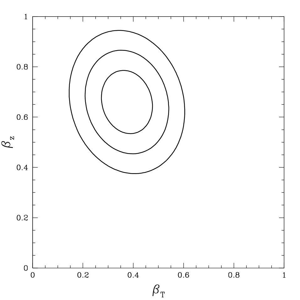
where , and are constants to be determined employing a minimum algorithm and is expressed in keV. The best fitting values are , and . Confidence intervals of the fitted values of and are shown in Figure 11. The minimum value of obtained using this procedure is approximately 3 per degree of freedom and, if the blue fraction errors are accurate, may indicate the presence of intrinsic scatter in the distribution of blue fraction values. The current sample of XMM-LSS and CCCP clusters is insufficiently large and does not cover a large enough interval in either redshift or temperature to constrain both the exponents of the redshift and temperature dependence of Equation 5 in addition to the coefficients. We can rule out no redshift evolution but the temperature dependence is relatively unconstrained (and is complicated by the degeneracy with as the power law exponent of tends to zero).
An alternative approach is to investigate the trends in the data employing a non-parametric approach. In this case we apply a partial Spearman rank analysis to the data in order to examine the extent of any correlation between and either temperature or redshift while controlling for the variation of the second variable. The partial correlation coefficient describing blue fraction and redshift while controlling for temperature is while the corresponding coefficient describing blue fraction versus temperature while controlling for redshift is . The probability of obtaining from the sample by chance is approximately 0.2% whereas the corresponding probability for the value is somewhat greater at approximately 1.8%. Overall, both the parametric and non-parametric approach confirm the evolution in the cluster blue fraction with both redshift and cluster temperature. The significance of the greater blue fraction versus decreasing temperature can also be seen in Figure 13 where the average blue fraction for the cool sample is significantly higher than either the blue fraction for the mid and hot samples.
One may further investigate the dependence of blue fraction on cluster temperature by correcting values for individual clusters to a common epoch at using Equation 5 and the best-fitting coefficients. The corrected values are displayed in Figure 12 and confirm the trend to observe greater blue fraction values in cooler clusters.

We consider further the implications of this trend in Section 6. We next consider the effects of the various choices made during the blue fraction analysis on the overall robustness of the blue fraction trends versus redshift and temperature.
4.1 Testing the blue fraction computation assumptions
The cluster blue fraction may be computed employing one of a number of crtieria to segregate the red and blue cluster galaxy populations. We apply the original definition of Butcher & Oemler (1984) in this paper but note the critiscisms of Andreon (2005) who argue that adopting a fixed rest frame colour offset relative to the red sequence is prone to give misleading blue fraction trends as galaxies of different SEDs drift in and out of the adopted colour interval as a funtion of redshift. To assess whether this is an important consideration in our analysis we compare the average blue fraction per cluster sub-sample to a modified blue fraction determined by fitting the red fraction associated with the stacked CMD of clusters by temperature. We follow the method described by Loh et al. (2008) and model the red wing of the red sequence of the CMD of all clusters stacked by temperature once -corrected to a common redshift (we defer the description of the stacking procedure to Section 5). The red wing is modelled as a double Gaussian function and the best-fitting function is reflected about the location of the red sequence to determine the number of red galaxies in each distribution. We then compute the red fraction in an analogous manner to the blue fraction and define a modified blue fraction as . We compare the original and modified blue fraction values for each temperature sub-sample in Figure 13 and note that each approach reveals the same trend (and that the points are identical within the errors). We are therefore satisfied that the original BO84 definition produces reliable results and we avoid the requirement to fit double Gaussian features to individual cluster colour distributions which, in the case of the cool clusters, typically result in poorly constrained models.

| Cluster | Number of blue galaxies | |
|---|---|---|
| XLSSC 13 | 11 | |
| XLSSC 51 | 11 | |
| XLSSC 44 | 13 | |
| XLSSC 08 | 14 | |
| XLSCC 40 | 5 | |
| XLSSC 23 | 16 | |
| XLSSC 22 | 10 | |
| XLSSC 25 | 17 | |
| XLSSC 18 | 14 | |
| XLSSC 27 | 12 | |
| XLSSC 10 | 20 | |
| MS0440+02 | 16 | |
| A1942 | 49 | |
| A0223 | 30 | |
| A2259 | 50 | |
| A1246 | 30 | |
| A2537 | 54 | |
| A0959 | 25 | |
| A0586 | 39 | |
| A0115 | 38 | |
| A0611 | 65 | |
| A0521 | 55 | |
| A2261 | 80 | |
| A2204 | 35 | |
| MS1008-12 | 58 | |
| CL1938+54 | 95 | |
| A0520 | 43 | |
| A1758 | 52 | |
| A2111 | 26 | |
| A0851 | 97 | |
| A0697 | 54 | |
| A2104 | 24 | |
| A1914 | 35 | |
| A2163 | 69 |
We next consider the variation of the computed blue fraction with assumed cluster radius to a) investigate whether the choice of radius introduces a bias into the trend of observed blue fraction versus temperature, b) determine the effect of uncertainty in the estimated value for each cluster on and c) relate blue fractions computed for the current sample to comparable studies in the literature. Figure 14 displays the average blue fraction per temperature sub-sample computed within circular apertures of radius expressed as a fraction of . This variation of the blue fraction with characteristic radius has been noted in previous studies and the trend displayed in Figure 14 are consistent with those of Fairley et al. (2001), Ellingson et al. (2001) and Wake et al. (2005). Though we discuss this trend further in Section 6 we note here that the increasing trend of blue fraction with scaled aperture radius is nominally consistent with a blue infalling field population that is processed by ram pressure stripping upon falling into each cluster. However, the details of this conclusion will be discussed in Section 6. The average blue fraction at in each temperature sub-sample reflects the trend observed in Figure 10. What can be noted at this point is that the exact choice of radius wihtin which blue fractions are computed does not affect the conclusion that cooler clusters display greater blue fractions than hotter clusters (within the range investigated here)44 4 Furthermore, we note that the value of in each case is computed employing the observed cluster temperature and an assumed mass-temperature relation. X-ray spectral measurements from which the cluster temperature is computed are typically extracted within an on-sky aperture of size of the order of in each cluster. Therefore, employing computed values to define aperture sizes up to several times the virial radius would invlove a considerable extrapolation beyond the scale on which the X-rays are measured..
Uncertainty in the temperature computed for each cluster propagates to an error in the value of computed for each cluster. The typical temperature error for the XMM-LSS clusters contributing to the cool sample are of the order of 10-20% (Willis et al. 2005). The gradient of the trend of versus estimate at is approximately 0.15. This indicates that uncertainty in cluster X-ray temperature will contribute a fractional error of order a few percent, i.e. small compared to the Poissonian error in computed for an individual cluster.

The mid temperature CCCP cluster MS1008 is common to both this work and that of Kodama & Bower (2001) and provides a useful check upon our results. The value of the blue fraction obtained by these authors was and was calculated within (the radius containing 30% of the total number of galaxies in the cluster) corresponding to an angular radius of 2.82′. We obtain a value within corresponding to an angular radius of 4.44′. The radial cut used by Kodama & Bower (2001) corresponds to approximately and when the blue fraction was recalculated within this fraction of , a value of was obtained, improving the agreement with Kodama & Bower (2001). We note that the errors quoted here are purely Poissonian and do not account for the effect that minor differences in the methodology used in each study (e.g. -correction, computation of the red sequence relation) have upon the computed value of .
We next consider the effect of extending the faint absolute magnitude cut applied when computing the blue fraction. Figure 15 displays the average blue fraction per temperature sub-sample computed within a circular aperture of as the applied faint magnitude cut is varied from to -18. The main feature of the diagram is that the excess fraction of blue galaxies observed in cool clusters compared to the mid and hot samples continues to increase as the sample magnitude limit is extended to fainter magnitudes.

When considered together, the variation of blue fraction with both radius and magnitude indicate that the excess blue galaxy fraction observed in cool clusters is dominated by the contrubtion of faint galaxies at large radius. In the following section we attempt to identify this population directly on the colour-magnitude diagram for each temperature sub-sample.
5 Stacked Colour Magnitude Diagrams
The previous analyses have identified a relative excess in the fraction of blue galaxies in cool X-ray clusters compared to the mid and hot samples. While the blue fraction is a useful quantity to investigate, it may prove informative to consider the average CMD for each temperature sample for which blue fractions are computed. The statistical background subtraction method described in Section 3 was applied 100 times to each cluster and the average CMD was computed by stacking the individual CMDs on a binned colour magnitude plane in intervals of 1 mag. in magnitude and 0.5 mag. in colour. The average background subtracted CMD for each cluster was then transformed to a common redshift . The transformation described the effects of distance dimming and the -correction. The -correction for each colour pixel on the CMD plane was computed using the best-fitting interpolated spectral template required to reproduce the required observed colour value at the cluster redshift. Individual cluster CMDs within each temperature sub-sample were then stacked on the CMD plane. Each cluster CMD was assigned equal weight in the stacking process by normalising all transformed CMDs to a total contribution of unity summed withing the region and . The stacked colour magnitude diagrams for each sample are shown in Figure 16. In addition, the fourth panel in Figure 16 indicates the result of subtracting the mid cluster stacked CMD from the corresponding cool cluster sample to highlight the location on the CMD of the excess fraction of blue galaxies found in the cool sample. As indicated in the plots, the relative excess appears uniform across a range of colours bluer than the red sequence. There is some evidence for an excess of faint () blue () galaxies in the cool sample. However, the CFHTLS optical data used to construct the cool CMD begins to be incomplete at these magnitudes and the purely visual impression may be flawed.

An alternative approach is to consider the colour distribution of all galaxies brighter than some limit. The colour distributions derived from the unweighted sum of all clusters in each temperature sample (corrected to ) are shown in the upper three panels of Figure 17. The limiting magnitude is , approximately equal to at this redshift. In order to investigate the distribution of blue galaxies in each sample the red sequence was modelled and removed in each case. Following Loh et al. (2008) the red wing of the red sequence was fitted using a double Gaussian model with the mean of each Gaussian set to the location of the red sequence and the best fitting full-width at half-maximum (FWHM) and normalisation of each profile determined using a minimum algorithm. The resulting model is then reflected about the location of the red sequence and subtracted from the corresponding colour distribution.
The mean colour of all galaxies bluer than the location of red sequence for each sample was calculated and found to be 0.70, 0.675 and 0.675 for the cool, mid and hot samples respectively. We hesitate to place too much emphasis on the trend to observe redder mean colours in the blue cloud for lower temperature X-ray systems. This is principally due to potential limitations such as a) the obvious subtraction artefact in the mid sample red sequence subtracted distribution and b) the broad nature of such peaks and the low number of galxies involved (in the cool systems).
The red sequence subtracted distribution for the cool sample does appear to show a population of extremely blue galaxies not seen in the corresponding mid and hot cluster samples. To quantify this additional population we define the extremely blue fraction to be the fraction of galaxies bluer than the colour of an Sc galaxy ( at ) for all galaxies down to for each sample. These extreme blue fractions were found to , and for the cool, mid and hot samples respectively. It was noted in Figure 15 that the fraction of blue galaxies in the cool cluster sample increases with the increasing faint magnitude limit used to define the blue fraction. With this in mind we computed the extremely blue fraction for the cool sample using galaxies in the magnitude range as shown in Figure 18. The computed extreme blue fraction is equal to , i.e. the population of extremely blue galaxies increases with increasing magnitude.


6 Discussion
We have presented an analysis of the fraction of blue galaxies in a large sample of X-ray clusters spanning a wide range of X-ray temperature with uniform optical photometry. We have noted that the computed blue fraction values display a trend to decrease with both decreasing redshift and increasing temperature.
The trend of decreasing cluster blue fraction versus redshift has been observed previously and has been interpreted as a global effect driven by the decreasing rate of field galaxy infall onto the cluster environment (e.g. Ellingson et al. 2001). Coupled with the increasing cluster mass with decreasing redshift, the specific infall rate per unit cluster mass decreases at an even faster rate. Infall effects are further compounded with the sharply declining global star formation rate as a function of decreasing redshift (Hopkins & Beacom, 2006) which may be viewed as a decrease in the available gas supply of infalling galaxies. Looking beyond the redshift dependent component of the Butcher-Oemler effect, the decreasing blue fraction with increasing X-ray temperature identified in this paper is consistent with an environmental component to the Butcher-Oemler effect.
The trend of decreasing blue fraction versus temperature is most apparent whan comparing the across XMM-LSS and CCCP samples rather than within either sample. It remains possible that this difference is due in part to some subtle selection effect arising during the construction of the two samples rather than as a result of some physical process linked to the global environment. However, it is not clear what form such a bias would take. At this point we recall that the cool clusters may display a mild bias to higher gas densities or more centrally concentrated systems compared to the average population. One would naively expect such systems to be more effective at processing infalling field galaxies compared to the average (i.e. lower X-ray luminosity) cluster over the same temperature interval – effectively introducing a mild bias toward lower blue fractions in this temperature sub-sample. One could therefore argue that access to a more complete census of the low-temperature cluster population would only amplify the trend of blue fraction versus temperature. It has also been noted that optically selected clusters display different optical properties compared to X-ray selected samples (see Haines et al. 2009 for a discussion). However, X-ray samples of bright clusters are typically complete in terms of the optical properties they sample (mainly because bright X-ray clusters are rare and thus it is possible to select complete samples). Moreover, clusters selected by single band optical observations (i.e. purely based upon the projected overdensity of bright galaxies) are more likely to be biased toward high blue fraction values due to the high mass-to-light ratios of blue star forming galaxies. We therefore note that any possible bias between the XMM-LSS and CCCP samples would be naively be expected to generate the opposite trend to that observed in this paper and we remain confident that the trend of blue fraction versus temperature we have identified is not a result of sample selection effects.
A currently favoured explanation for the observed trend of blue fraction versus temperature is that infalling field galaxies are processed physically as they interact with the cluster environment. This interaction may take the form of ram pressure stripping whose effectiveness is a relatively simple function of the mass scale represented by the group or cluster into which the galaxies are falling. An alternative explanation is that infalling galaxies are processed via galaxy-galaxy interactions and therefore respond more readily to a combination of local rather than global velocity dispersion and galaxy density. Whatever the cause, it is clear that the process by which blue galaxies are processed to appear red is more complete in hotter (more massive) environments compared to cooler (less massive) environments.
Disentangling the above two effects is difficult as, to first order, the effects upon star formation in the infalling galaxy depend on environment in the same manner: ICM stripping and subsequent SF suppression are expected to be weakest (though not absent) in group environments – galaxy populations in these environments will display a larger fraction of blue galaxies relative to more massive clusters – while SF enhancements associated with galaxy-galaxy interactions will be greater on group scales. Each effect would naively generate the same observed trend of blue fraction versus temperature.
The blue fraction in each temperature sub-sample displays a very similar trend versus scaled radius and is consistent with an infalling field population albeit the cool sample is offset to higher blue fraction (Ellingson et al., 2001). However, the cool sample displays a marked increase in blue fraction with decreasing magnitude. The increase in the cool sample blue fraction with increasing magnitude results from both a moderate increase in the number of blue galaxies but also in a relative deficit in the numbers of red galaxies compared to those in the mid and hot samples. We will address the red sequence luminosity function of the cool, mid and hot samples in a subsequent paper. However, we note that the relative deficit of red galaxies in cool clusters compared to the mid and hot samples is consistent with the scenario where the processing of blue galaxies to red galaxies during infall is relatively incomplete.
Having subtracted the red sequence contribution from each colour histogram the blue galaxy colour distribution for each temperature sub-sample appears very similar. We do note an excess of extremely blue galaxies in the cool sample compared to the mid and hot samples. The excess is small (an extremely blue fraction of 3% compared to ) yet significant. In addition the fraction of extremely blue galaxies increases in the cool sample from to for galaxies displaying and respectively. One may tentatively associate these galaxies as actively star-bursting galaxies potentially driven by galaxy-galaxy interactions (e.g. De Propris et al. 2003). De Propris et al. (2003) comment that the absence of a strong Butcher-Oemler effect in near-infrared selected cluster galaxy populations compared to optically selected populations may be due to an increasing contribution from faint blue dwarfs whose optical brightness is boosted by recent star formation. The extremely blue population identified in the cool sample is nominally consistent with this explanation yet clearly forms only a small component of the overall blue cluster galaxy population. The small relative contribution of such potentially star bursting galaxies to the cluster population may be understood in terms of the short timescale over which a recent star burst will affect the integrated colour of an established stellar population. This issue has been addressed by Barger et al. (1996) who simulate the colour evolution with time of an underlying passive (elliptical-type) and continuous star formation (spiral-type) stellar population experiencing a short ( Myr), secondary ( by mass) burst of star formation associated with an interaction resulting from the cluster environment. The shift towards bluer colours as a result of a moderate burst of star formation lasts typically only as long as the burst duration before the luminosity weighted colour reverts to that of the underlying pre-burst stellar population. The effect is more pronounced when one applies the condition that all star formation ceases after the secondary burst, in which case the continuously star forming stellar population (spiral-type) reddens to approximately the same colour as the passive population within Gyr of the burst.
Our analysis has identified a clear environmental dependence in the blue fraction of galaxies. However, the cause of this environmental Butcher-Oemler effect – whether it be ram pressure stripping or galaxy-galaxy interactions – cannot be discerned unambiguously on the basis of the colour distribution of the blue galaxy population in each sample. Clearly further information is required, most notably the combination of colour information with morphological information. One would naively expect the above two environmental processes to affect galaxy morphology in markedly different ways, e.g. ram pressure effects hould not disrupt galaxy disks whereas a strong disruptive effect is expected from galaxy-galaxy interactions. We will present this investigation in a future paper.
Acknowledgments
The authors wish to thank Graham Smith, Michael Balogh, Stefano Andreon, Pierre-Alain Duc, Florian Pacaud and Kevin Pimblett for providing useful comments during the development of this paper. SAU and JPW acknoweldge financial support from the Canadian National Science and Engineering Research Council (NSERC).
References
- Abadi et al. (1999) Abadi, M.G., Moore, B., Bower, R.G., 1999, MNRAS, 308, 947
- Andreon et al. (2004) Andreon S., Lobo C., Iovino A., 2004, MNRAS, 349, 889
- Andreon (2005) Andreon, S., 2005, in The Fabulous Destiny of Galaxies: Bridging Past and Present, ed. V. Le Brun (Paris, Frontier Group)
- Andreon & Ettori (1999) Andreon, S., Ettori, S., 1999, ApJ, 516, 647
- Balogh et al. (1999) Balogh, M.L., Morris, S.L., Yee, H.K.C., Carlberg, R.G., Ellingson, E., 1999, MNRAS, 527, 54
- Barger et al. (1996) Barger, A.J., Aragón-Salamanca, A., Ellis, R.S., Couch, W.J., Smail, I., Sharples, R.M., 1996, MNRAS, 279, 1
- Berrier et al. (2009) Berrier, J.C., Stewart, K.R., Bullock, J.S., Purcell, C.W., Barton, E.J., Wechsler, R.H., 2009, ApJ, 690, 1292
- Bertin & Arnouts (1996) Bertin E., Arnouts S., 1996, A&AS, 117, 393
- Bildfell et al. (2008) Bildfell C., Hoekstra H., Babul A., & Mahdavi A., 2008, MNRAS, 389, 1637
- Blanton et al. (2005) Blanton, M.R., Eisenstein, D., Hogg, D.W., Schlegel, D., Brinkmann, J., 2005, ApJ, 629, 143
- Butcher & Oemler (1984) Butcher, H., Oemler, A., 1984, ApJ, 285, 426
- Cox et al. (2008) Cox, T.J., Jonsson, P.,Somerville, R.S., Primack, J.R., Dekel, A., 2008, MNRAS, 384, 386
- Chung et al. (2007) Chung, A., van Gorkum, J.H., Kenney, J.D.P., Vollmer, B., 2007, ApJ, 659, L115
- De Propris et al. (2003) De Propris R., et al., 2003, MNRAS, 342, 725
- Di Matteo et al. (2007) di Matteo, P., Combes, F., Melchior, A.-L., Semelin, B., 2007, A&A, 468, 61.
- Dressler et al. (1994) Dressler, A., Oemler, A., Sparks, W.B., Lucas, R.A., 1994, ApJ, 425, L23
- Dressler et al. (1997) Dressler, A., Oemler, A., Couch, W.J., Smail, I., Ellis, R.S., Barger, A., Butcher, H., Poggianti, B.M., Sharples, R.M., 1997, ApJ, 490, 577
- Duc et al. (2002) Duc, P.-A., Poggianti, B. M., Fadda, D., Elbaz, D., Flores, H., Chanial, P., Franceschini, A., Moorwood, A., Cesarsky, C., 2002, A&A, 382, 60
- Ellingson et al. (2001) Ellingson, E., Lin, H., Yee, H.K.C., Carlberg, R., 2001, ApJ, 547, 609
- Fairley et al. (2001) Fairley B.W., Jones L.R., Wake D.A., Collins C.A., Burke D.J., Nichol R.C., Romer A.K., 2001, MNRAS, 330, 755
- Finoguenov et al. (2001) Finoguenov A., Reiprich T.H., Bohringer H., 2001, A&A, 368, 749
- Geach et al. (2009) Geach, J.E., Smail, I., Moran, S.M.. Treu, T., Ellis, R.S., 2009, ApJ, 691, 783
- Gunn & Gott (1972) Gunn, J.E., Gott, J.R., 1972, ApJ, 176, 1
- Haines et al. (2009) Haines, C. P., Smith, G. P., Egami, E., Ellis, R. S., Moran, S. M., Sanderson, A. J. R., Merluzzi, P., Busarello, G., Smith, R. J., 2009, ApJ, 704, 126
- Hansen et al. (2009) Hansen, S. M., Sheldon, E. S., Wechsler, R. H., Koester, B. P., 2009, ApJ, 699, 1333
- Hoekstra et al. (2006) Hoekstra, H., Mellier, Y., van Waerbeke, L., Semboloni, E., Fu, L., Hudson, M. J., Parker, L. C., Tereno, I., Benabed, K., 2006, ApJ, 647, 116
- Hopkins & Beacom (2006) Hopkins, A.M., Beacom, J.F., 2006, ApJ, 651, 142
- Horner (2001) Horner D., 2001, PhD thesis, University of Maryland
- Kawata & Mulchaey (2008) Kawata, D., Mulchaey, J.S., 2008, ApJ, 672, 103
- Kinney et al. (1996) Kinney, A. L., Calzetti, D., Bohlin, R. C., McQuade, K., Storchi-Bergmann, T., Schmitt, H. R., 1996, ApJ, 467, 38
- Kodama & Bower (2001) Kodama T., Bower R.G., 2001, MNRAS, 321, 18
- Li et al. (2009) Li, I.H., Yee, H.K.C., Ellingson, E., 2009, ApJ, accepted.
- Loh et al. (2008) Loh, Y.-S., Ellingson, E., Yee, H.K.C., Gilbank, D.G., Gladders, M.D., Barrientos, L.F., 2008, ApJ, 680, 214
- Makino & Hut (1997) Makino, J., Hut, P., 1997, ApJ, 481, 83
- Margoniner et al. (2001) Margoniner, V. E., de Carvalho, R. R., Gal, R. R., Djorgovski, S. G., 2001, ApJ, 548, L143.
- McCarthy et al. (2008) McCarthy, I.,G., Frenk, C.S., Font, A.S., Lacey, C.G., Bower, R.G., Mitchell, N.L., Balogh, M.L., Theuns, T., 2008, MNRAS, 383, 593
- Moore et al. (1996) Moore, B., Katz, N., Lake, G., Dressler, A., Oemler, A., 1996, Nature, 379, 613
- Oemler et al. (2009) Oemler, A., Dressler, A., Kelson, D., Rigby, J., Poggianti, B.M., Fritz, J., Morrison, G., Smail, I., 2009, ApJ, 693, 152
- Pacaud et al. (2007) Pacaud F., Pierre, M., Adami, C., et al., 2007, MNRAS, 382, 1289
- Poggianti et al. (1999) Poggianti, B.M., Smail, I., Dressler, A., Couch, W.J., Barger, A.J., Butcher, H., Ellis, R.S., Oemler, A., 1999, ApJ, 518, 576
- Poggianti et al. (2006) Poggianti, B., et al., 2006, ApJ, 642, 188
- Pimbblet et al. (2002) Pimbblet K.A., Smail I., Kodama T., Couch W.J., Edge A.C., Zabludoff A.I., O’Hely E., 2002, MNRAS, 331, 333
- Saintonge et al. (2008) Saintonge, A., Tran, K.-V.,H., Holden, B.P., 2008, ApJ, 685, L113
- Treu et al. (2003) Treu, T., Ellis, R.S., Kneib, J.-P., Dressler, A., Smail, I., Czoske, O., Oemler, A., Natarajan, P., 2003, ApJ, 591, 53
- van Dokkum et al. (1999) van Dokkum, P.G., Franx, M., Fabricant, D., Kelson, D.D., Illingworth, G.D., 1999, ApJ, 520, L95
- Wake et al. (2005) Wake, D.A., Collins, C.A., Nichol, R.C., Jones, L.R., Burke, D.J., 2005, ApJ, 627, 186
- Willis et al. (2005) Willis J.P., Pacaud, F., Valtchanov I. et al., 2005, MNRAS, 363, 675
- Wolf et al. (2009) Wolf, C., et al., 2009, MNRAS, 393, 1302