Universal States in Layered Systems of Cold Polar Molecules Ultracold gases, trapped gases Macromolecules and polymer molecules Quantum statistical mechanics
Bound States and Universality in Layers of Cold Polar Molecules
Abstract
The recent experimental realization of cold polar molecules in the rotational and vibrational ground state opens the door to the study of a wealth of phenomena involving long-range interactions. By applying an optical lattice to a gas of cold polar molecules one can create a layered system of planar traps. Due to the long-range dipole-dipole interaction one expects a rich structure of bound complexes in this geometry. We study the bilayer case and determine the two-body bound state properties as a function of the interaction strength. The results clearly show that a least one bound state will always be present in the system. In addition, bound states at zero energy show universal behavior and extend to very large radii. These results suggest that non-trivial bound complexes of more than two particles are likely in the bilayer and in more complicated chain structures in multi-layer systems.
pacs
67.85.-dpacs
36.20.-rpacs
05.30.-d1 Introduction
Quantum gases of polar atoms and molecules in their rovibrational ground-state represent a unique opportunity to study the interplay of long- and short-range interactions in the highly controllable trapped gas environment. Early experiments used magnetic dipolar atoms [1, 2, 3, 4] which have observable effects in spite of intrinsically weak dipole moments. Recently, heteronuclear molecules with very large electric dipole moments have been realized by a number of groups [5, 6, 7, 8, 9]. The goal of a quantum degenerate system of polar molecules with strong long-range dipole-dipole forces therefore seems close at hand.
The attractive force of polar molecules in the head-to-tail configuration can lead to collapse of the system [10]. However, as suggested by Wang et al. [11], a one-dimensional optical lattice that creates a multilayered stack of pancake systems can stabilize the situation. If we apply a field to polarize the dipoles perpendicular to the layers then the intralayer interaction will be purely repulsive, whereas the interlayer part will be attractive but with the optical lattices separating the dipoles in different layers. This setup is presently being implemented experimentally. As discussed in [11], the dipole-dipole force forms bound chains and the system effectively behaves as a liquid of chains with resemblance to rheological fluids. In the case of bosons we expect the chains to Bose condense at low temperatures. However, if we have fermionic polar molecules the situation is less clear since one would expect a Bose-Fermi mixtures with various bound complexes [12]. The dipole potential can also now be inverted to have a repulsive core with the use of laser fields [14, 13], which offers different physics possibilities than the “natural” dipole orientation.
If we simplify the problem to consider just two adjacent layers we have a system with interactions that mimics the long-range interactions in graphene [15] and semiconductor bilayers [16]. In the semiconductor case bound states of exciton pairs with non-zero dipole moments have been considered in connection with organic interfaces and quantum wells [17]. For small coupling strength it was concluded that no bound state exists [17]. This was also stated in several recent works concerning cold polar molecules [11, 18, 12] where the conclusion was based on a Gaussian ansatz. However, at small coupling the particles are strongly delocalized and a localized Gaussian is therefore not a good approximation [19]. To make matters worse, the potential integrates to zero over the plane and thus at small coupling the Landau criterion [20] for a bound state in two-dimensional systems is not applicable. Using scattering theory it was recently shown that a bound state presumably exists for arbitrarily small moments [21, 22]. However, the scattering theory is intricate and does not yield straightforward information about the behavior of the two-body bound state wave function.
The purpose of the present work is to compute and explain the basic properties of two-body systems used as the fundamental building blocks for layered dipolar structures. We shall employ simple model potentials to extract universal properties, point out where details of the potentials are needed, and illustrate relations between wave functions, energies, and radii. We shall use square well, harmonic oscillator and -potentials in two dimensions, and compare to solutions of the true dipole-dipole potential. We briefly sketch the model solutions, discuss energies, threshold properties, and various implications.

2 Model solutions
We solve the 2-dimensional (2D) Schrödinger equation, which is possible to do analytically with several model potentials. We use cylindrical coordinates and separate the total wave function into radial and angular parts. With , where is an integer, the stationary radial Schrödinger equation becomes:
| (1) |
where is the reduced radial wave function, is the energy, and is the potential, assumed to be spherically symmetric. We consider potentials with net volume equal to zero, , just as for the dipole-dipole potential, i.e.
| (2) |
where is the electric dipole moment and is the distance between the two different layers containing the particles. This potential is in Fig. 1 compared with square well, harmonic oscillator, and potentials at distances less than their common node at . The equal volume conditions relate strengths and shifts for given radial shapes. Thus we have , and for the square well shape, the small, , and large, , distance absolute strength values are related by
| (3) |
where is the radius where the outer square well ends. The attractive part is the most interesting and we shall only use the harmonic and potentials with the square barrier shape for as illustrated in Fig. 1.
One of our main concerns is the appearance of a bound state at small couplings. We therefore only consider the most attractive potential which simplifies to
| (4) |
where depends on .
Let us now first solve completely the piecewise constant potential in Fig. 1 for use as a reference standard. Then the wave functions in the three different regions of space are the Riccati Bessel functions of order , which means that the solutions for are various Bessel functions of order 0 depending on the region of space:
| (5) |
where are ordinary and modified Bessel functions of the first and second kind, respectively. The coefficients and are determined by matching at the region boundaries and by normalization. The wavenumbers, , are the absolute values of in the regions. Matching logarithmic derivatives leads to the transcendental equation for the energies:
| (6) |
This formula and the wave function, Eq.(5), are valid for the potential in Fig. 1. For from Fig. 1, one merely takes the analytic continuation of the relevant Bessel function. Expanding the solution for small strengths results in
| (7) |
where . Eq.(7) with the second order potential strengths replaces the Landau expression when the potential integrates to zero[20].
Analytic solutions can also be found when the short-distance part of the potential is substituted by a harmonic oscillator potential, and a potential, . In both cases the potentials are zero for and is the strength of the box potential with the same volume below . The radial wave functions for are given by , where is the confluent hypergeometric function, or Kummer function with three arguments. We have and and are:
| (8) | |||||
| (9) |
for oscillator and potentials, respectively. This is the solution vanishing at . Matching at with the square well solutions for leads to trancendental equations for the energies.

3 Energies
The energies obtained from Eq. (6) are shown in Fig. 2 as function of , or equivalently of volume of either attraction or repulsion. We choose or , as indicated, and use from Eq.(3). Increasing for both natural and inverted potentials leads to more bound states which more and more are determined from the attraction alone and independent of the confining barriers. The condition, , determines for in Fig. 1 and thereby the bound state energy is related to the nodes of the Bessel function, i.e.
| (10) |
where is the th zero of . This asymptotic limit of straight lines of slope equal to one is valid for an infinitely high barrier. The ground state is the deepest and agrees well with the asymptotic limit, but for the excited states the well must be deeper to reach the limit, around -150 for 1% agreement for the first excited state.
For in Fig. 1, where the repulsion is for and the attractive well is at , no confining barrier exists at larger distance. Here, the bound state wave function is where is the Neumann function. In the deep well limit, the wave function must vanish at both endpoints where large energy implies large arguments of both the Bessel and Neumann functions. Then or equivalently
| (11) |
where the slopes of the lines are dependent on and therefore different from the case. These estimates are much further off than the similar estimates for . For the difference between the energies and the estimate to be 1% for the ground state, the depth of the well needs to be around 100. For that level of agreement in the first excited state, the well depth needs to be around 250.
The result for small strengths are shown in the inset of Fig.2. One bound state is always present for all potentials even when the strength is approaching zero. The dependence on both strengths and radius () is substantially stronger for the inverted potentials. The very small energies close to threshold obey the limiting linear dependence from Eq. (7). They are extremely small due to the zero net volume, and hence difficult to obtain accurately. The numerical results for the dipole potential almost coincide with the energies for the other potentials. On the scale of the inset the energies are exceedingly small and difficult to calculate numerically, especially for the inverted dipole potential. For larger strengths on the inverted side and on the natural side, we found that the energies rather precisely are given by , where for the natural and inverted potentials, respectively.
The values in the experiments [6] correspond to strengths of about or (Fig. 2) which is on the verge of universality (see Fig. 4), although current temperatures are too high to maintain such a weakly bound state [6]. Fortunately, systems with larger can be explored where the bound state energy is much larger and obeys the analytic formula given above.

These computations are also carried out for harmonic oscillator and potentials at small distance with a square well at larger distances. The condition of exponentially vanishing wavefunction with implies that the first argument of the Kummer function must be a non-positive integer counting the bound states. Then reduces to the Laguerre polynomials. The energies become
| (12) | |||||
| (13) |
where can take the values 0,1,2, etc. These energies are only approached asymptotically as for the square well in Fig. 1. They are highly potential dependent for well-bound states as the barrier essentially has no influence on these energies, see Fig. 3. The potential in Eq.(2) leads to energies between those of harmonic and square well potentials. Thus limits to realistic potentials can be provided by analytic models.
However, in the limit where both energies in Eqs.(12) and (13) approach zero from positive values. The approximations are too crude, and we replace the potentials by the corresponding square well. We then find numerically that the energies for both these potentials always remain negative corresponding to bound states for all values of . Thus all the investigated potentials with zero net volume always have at least one bound state.
4 Threshold properties
The weakly bound states often reveal unique physics as for example Efimov and halo states with universal properties. The number of nodes as function of volume can be found rather precisely from Eqs.(10-13) by solving for with . The explicit result for harmonic oscillator, , whereas for the potential the right-hand side is a factor larger. Thus these potentials would have the same number of bound states if the volume of the oscillator were twice as large as that of the -potential. The dipole-dipole potential seems from Fig. 1 to have intermediate properties. However, the dependencies on strength for each energy differs substantially, see Eqs.(12) and (13).
The same extrapolation to the threshold can be applied to the wave functions. We then find that the mean square radius is given as for the oscillator and to leading order for the potential. These threshold radii, obtained from asymptotic strong binding, are however qualitatively completely wrong when the energy is sufficiently close to zero. In Fig. 2 the straight lines approaching zero bend over as the system attempts to stay bound for a weaker potential. The wave function is correspondingly leaking out under the barrier as the energy approaches zero. This is the effect producing nuclear halos [19] where the mean square radius for two particles in three dimensions becomes inversely propertional to the energy. The analogue here is that most of the probability is found for where the wave function is . This means that the mean square radius then approaches [23]
| (14) |
which is a universal result independent of both the particular (-wave) state considered and the shape of the attractive potential.
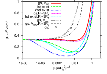
The rate of approach to the asymptotic value in Eq.(14) is seen in Figure 4. Large binding energies correspond to wave functions located in the attractive well. As the threshold is approached the wave function begins to leak out and eventually ends up in the universal limit in Eq.(14). However, how that limit is approached depends on the presence of a barrier. Without a barrier ( from Fig. 1), all states, both ground and excited, approach the weak binding limit in the same way. This is precisely the halo effect [19].
The similar approach to universality is found for the ground state for from Fig. 1 since then the barrier vanishes with the binding energy. For excited states of , the barrier remains finite for vanishing binding energy. High excitation goes together with high barrier which causes even the weakly bound states to remain localized in the attractive region. The approach to universality is delayed by many orders of magnitude in binding energy. During the approach the radius remains small for small energies and consequently the curves dive below the universal limit before the eventual approach. These features become more pronounced with excitation energy.
In Figure 4 we also show results for different values of , still with adjusted to maintain zero net volume. The curves for the ground states are roughly identical. This is also seen at higher energies for the first excited state, but eventually at small energies a wider barrier delays the escape of the wave function even though the barrier is correspondingly smaller.
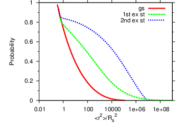
The rate of approach to the universal limit at threshold is further illustrated in Figure 5. The probability distribution from the wavefunction is moving slower than the distribution in the mean square radius integral. The bulk of the probability can stay in the attractive well while the root mean square radius is much larger than the radius of the attraction. Thus the tail properties are crucial. These effects are enhanced for excited states because the final expulsion of the wave function to the external region comes much later for states constraint by a large barrier.
The formal connection is that the wave function essentially is until the energy is very small where it has to change to , see Eq.(5). Computation of mean square radius then employs for normalization but for the -distribution. Thus neither short nor large-distance properties are sufficient for a description in this transition region.
5 Implications for many particles
Several conclusions are immediately deduced from our model systems. First of all, at least one bound state must appear in 2D for any potential with zero net volume. Thus, in contrast to the statements in [17, 11, 18, 12], one bound state is always present in a bilayer with dipoles oriented perpendicular to the layers. This in turn means that arguments based on the existence of a critical strength for binding should be re-considered. Furthermore, since a large dipole moment implies a large strength, several two-body bound states will be present. This must be taken into account in simulations of configurations of actual systems where a finite temperature might lead to population of different excited states. In practice, finite temperature in the system will put a natural limit on how small binding energies one needs to consider, i.e. for the bound states are thermally dissociated into the continuum and therefore largely irrelevant.
Second, a positive net volume still allows bound states in two dimensions. However, now it is necessary to have a non-zero minimum attraction where the strength would increase with the net volume. This resembles the situation in three-dimensional quantum mechanics.
Third, the structure of many particles in layers are strongly influenced by their pair interactions. The absence of a critical interaction strength for binding implies that a phase transition from a superfluid to a dipolar chain liquid cannot occur in contrast to the suggestion in [11, 18]. Furthermore, the presence of bound states in bilayers for all strengths immediately implies that chains in multilayers will also be present for all couplings. We would therefore expect the system to always be a dipolar chain liquid. As all the individual chains can form immediately the chain-chain interaction becomes interesting and necesary to include in careful future investigations.
We can in fact give an upper bound on the binding energy of a chain of particles in different layers. The scaling of two-body energy with layer distance is , with an integer giving the distance in equally spaced layers a distance apart. Here is the two-body energy we have calculated above which depends on the coupling strength. Taking the large limit, the upper bound is
| (15) |
This estimate of the energy agrees well with the calculation of [11] where the harmonic approximation was at small couplings for and .
Fourth, the inverted potential with in Fig. 1 with repulsion at small distances and an intermediate attractive pocket also has at least one bound state for any strength. In the bilayer system with a finite density of fermionic polar molecules in each layer, Ref. [13] found an interesting particle-hole coherent state. The density used there was chosen small so intralayer interaction is negligible and the focus was on the interlayer repulsion corresponding to a barrier at small radii and an attractive pocket outside. In [13] the presence of bound states shown in this paper was ignored. In a real system at finite temperature this coherent state could probably exist at low dipole strength. However, at larger strengths the bound states must be taken into account and one would presumably have instead an interacting gas of bound pairs behaving as a superfluid.
Fifth, the bound states become extremely extended as the energy gets sufficiently close to zero. Such delocalized two-body states can in turn enter into complicated multi-particle complexes[24]. A bound three-body system of two particles in one plane and one in between in the adjacent plane is therefore possible. This presupposes that the repulsive intraplane interaction between these extended structures is less than two times the two-body binding energy that created the two-body bound states. This sort of Y-junction configuration can be very interesting in thermodynamic considerations of chains as it will contribute non-trivially to the entropy and can help lower the free energy. Full quantum studies of such configurations are therefore very relevant and worth pursuing.
Sixth, the optimum conditions for interesting multi-particle structures are probably in the regime close to the threshold for binding of the second state. This can be below the threshold where additional attraction from other particles would lead to binding in analogy to Borromean three-body systems where the two-body subsystems are unbound [23, 19]. It can also be for slightly larger attraction and with a bound two-body state since such a system still is spatially extended and in a sense rather similar to the unbound continuum state. The latter case is analogous to the extremely weakly bound atomic helium dimer where the trimer becomes well bound but with a very weakly bound and spatially extended excited state [23, 19].
Seventh, the regime of weak binding, strong delocalization and large root-mean-square radius exhibits universal features independent of the shape of the potentials. The same type of universality is likely to exist for multiple bound states but much finer tuning is probably required to reach these structures.
6 Conclusions
Presently experimentalists are working to produce layered systems of dipolar molecules. We use simple model potentials to study the bilayer case with dipoles polarized perpendicular to the layers. We find the solutions and calculate properties of the wave functions and in particular binding energies and radii as functions of dipole moment or strength of the potentials. Realistic potentials are used to test the generality of our results.
We conclude that there always is a bound state for all strengths of the dipole-dipole potential. We find that the wave functions of both ground and excited states show universal behavior at zero energy as they basically reside where the potential has become vanishingly small. To access this universal regime the dipole strength must be tuned around the threshold for a bound state to appear. The extended wave functions indicate that three or more particle complexes are possible in chains and in bilayers. The repulsive in-plane interaction becomes interesting in connection with these structures. In any case the tuning of interactions to universal regimes emphasizes the close analogy to the physics studied through the well-known technique of Feshbach resonances.
Acknowledgements.
NTZ is grateful to B. Wunsch, D.-W. Wang and E. Demler for numerous discussions.References
- [1] \NameGriesmeier A., Werner J., Hensler S., Stuhler J. Pfau T. \REVIEWPhys. Rev. Lett.942005160401.
- [2] \NameVengalattore M., Leslie S. R., Guzman J. Stamper-Kurn, D. M. \REVIEWPhys. Rev. Lett.1002008170403.
- [3] \NameFattori M. et al. \REVIEWPhys. Rev. Lett.1012008190405.
- [4] \NamePollack S. E. et al. \REVIEWPhys. Rev. Lett.1022009090402.
- [5] \NameOspelkaus S. et al. \REVIEWNature Phys.42008622
- [6] \NameNi K.-K. et al. \REVIEWScience3222008231
- [7] \NameDeiglmayr J. et al. \REVIEWPhys. Rev. Lett.1012008133004.
- [8] \NameLang F. et al. \REVIEWPhys. Rev. Lett.1012008133005.
- [9] \NameOspelkaus S. et al. \REVIEWScience1012010853.
- [10] \NameLushnikov P. M. \REVIEWPhys. Rev. A662002051601
- [11] \NameWang D.-W., Lukin M. D. Demler E. \REVIEWPhys. Rev. Lett.972006180413.
- [12] \NameKlawunn M., Duhme J. Santos L. \REVIEWPhys. Rev. A812010013604
- [13] \NameLutchyn R. M., Rossi E. Das Sarma S. \REVIEWarxiv:0911.1378v12009
- [14] \NameCooper N. R. Shlyapnikov G. V. \REVIEWPhys. Rev. Lett.1032009155302
- [15] \NameNovoselov K. S. et al. \REVIEWNature Phys.22006177
- [16] \NameYe J. \REVIEWJour. Low Temp. Phys.1582010882
- [17] \NameYudson V. I., Rozman M. G. Reineker P. \REVIEWPhys. Rev. B5519975214
- [18] \NameWang D.-W. \REVIEWPhys. Rev. Lett.982007060403.
- [19] A.S. Jensen, K. Riisager, D.V. Fedorov and E. Garrido, Rev. Mod. Phys. 76 (2004) 215-261.
- [20] \NameLandau L. D. Lifshitz E. M. \BookQuantum Mechanics \PublPergamon Press, Oxford \Year1977.
- [21] \NameShih S.-M. Wang D.-W. \REVIEWPhys. Rev. A792009065603
- [22] \NameTicknor C. \REVIEWPhys. Rev. A802009052702
- [23] \NameNielsen E., Fedorov D. V., Jensen A. S. Garrido E. \REVIEWPhys. Rep.3472001373
- [24] \NameB. Wunsch et al. \REVIEWin preparation2010