QCD with Chemical Potential in a Small Hyperspherical Box
Abstract:
To leading order in perturbation theory, we solve QCD, defined on a small three sphere in the large and limit, at finite chemical potential and map out the phase diagram in the plane. The action of QCD is complex in the presence of a non-zero quark chemical potential which results in the sign problem for lattice simulations. In the large theory, which at low temperatures becomes a conventional unitary matrix model with a complex action, we find that the dominant contribution to the functional integral comes from complexified gauge field configurations. For this reason the eigenvalues of the Polyakov line lie off the unit circle on a contour in the complex plane. We find at low temperatures that as passes one of the quark energy levels there is a third-order Gross-Witten transition from a confined to a deconfined phase and back again giving rise to a rich phase structure. We compare a range of physical observables in the large theory to those calculated numerically in the theory with . In the latter case there are no genuine phase transitions in a finite volume but nevertheless the observables are remarkably similar to the large theory.
Keywords:
QCD at finite chemical potential; perturbation theory; large N1 Introduction
The phase diagram of QCD at finite quark number density is of considerable interest but a first principles derivation of the grand potential has eluded us for two very good reasons. The first is that the phase transitions are conjectured to occur at densities where the coupling strength of QCD is large and thus the application of conventional perturbation theory is not valid. The other reason is that the action of QCD is complex resulting in the sign problem. This prevents the use of the usual technique of importance sampling in lattice gauge theory simulations as it is not possible to formulate a probability interpretation with a complex Boltzmann factor. However, there has been progress since several ways to work around the sign problem have been discovered, as will be discussed shortly. We propose a complementary idea which is to formulate the theory on a manifold with sufficiently small spatial volume such that perturbation theory is valid, and so that the calculation is valid at all temperatures and densities. Our particular choice of spatial manifold is , which is motivated by the connection with the AdS/CFT correspondence. In a nut-shell, when the maximally super-symmetric gauge theory is defined in a compact space, an , its thermodynamics in the large limit and at strong ’t Hooft coupling can be addressed by the dual gravitational description. What is remarkable is that the phase structure seems to match on to the weak coupling description that is addressed in perturbation theory; namely, as the temperature is raised there is a confinement/deconfinement type transition, a phase transition that is described in the gravity dual as a Hawking-Page transition from AdS space to an AdS black hole space [1, 2, 3]. This kind of analysis has been extended to include an -charge chemical potential [4]. What we take from this is that it is interesting to investigate the phase structure of any gauge theory in finite volume, on an , at weak coupling which is ensured if the size of the , , is much smaller than the strong coupling scale . In this case a thermodynamic limit is ensured by taking the large limit and genuine phase transitions occur. These transitions have all the characteristics of phase transitions that are expected in theories with finite defined on flat space. The goal of the present paper is to extend this kind of analysis to gauge theories with fundamental quarks in the large Veneziano limit [5], i.e. with the ratio fixed, with both finite temperature and baryon chemical potential. It will be interesting to relate our weak coupling results to strong coupling analysis based on the AdS/CFT correspondence. This will involve adding ‘‘flavour branes’’ to the basic set up to describe the quarks.11 1 The process of adding flavour to the basic AdS/CFT set-up has a huge literature. Most of this work addresses the case where the boundary theory is defined on and with fixed , so that the flavours can be introduced in the probe approximation; however, the papers [6, 7] consider the case of global with an boundary.
Our approach should have implications for understanding one of the outstanding problems in theoretical physics; namely, the behaviour of cold dense baryonic matter, which in essence corresponds to an understanding of QCD with non-zero baryon chemical potential . Its resolution would permit contact between particle and nuclear physics via a quantitative description of bulk nuclear matter from first principles, and would set the study of compact stars on a firm theoretical footing, via the input of the QCD equation of state (energy density , pressure ) into the Tolman-Oppenheimer-Volkoff equations for relativistic stellar structure. Indeed, such a programme is a necessary prerequisite for determining whether postulated ground states such as color-superconducting quark matter could ever exist in our universe.
The current consensus [8] is that as baryon density increases, the state best described as “nuclear matter”, viz. a degenerate system of neutrons and protons with fm-3 which is the favoured ground state once exceeds its onset value MeV, is somehow succeeded by an alternative degenerate system called “quark matter”. The properties of quark matter have been the subject of intense speculation over the past decade; it has been suggested that for sufficiently low temperatures , as a result of quark Cooper pair condensation at the Fermi surface, global, local and even translational symmetries may be spontaneously broken in the ground state, leading to exotic phenomena such as color superconductivity (CSC) or even crystallization [9]. From a theoretical standpoint these scenarios are most readily studied at weak coupling, which in the thermodynamic limit can only be quantitatively accurate at asymptotically high densities where , and yet the passage from nucleons to quarks referred to above clearly requires a non-perturbative treatment. At the very least, a reliable matching between perturbative and non-perturbative regimes is required. A recent calculation to this end has appeared in [10]. Other theoretical issues which naturally arise in this context include: what precisely is meant by “degenerate matter”? (this is usually taken to mean a system with a well-defined Fermi surface characterized by a momentum scale , but this definition is not gauge-invariant), and, does chiral symmetry restoration and/or deconfinement occur as increases? And, if so, to what extent do the transitions resemble those known to occur for as is raised?
An important reason why a non-perturbative understanding of QCD with has not progressed as much as in other areas is the unavailability of lattice gauge theory simulations performed using standard techniques [11]. A system with is not invariant under time reversal, since a bias is introduced in favour of particle propagation in the positive direction. In the Euclidean metric this results in asymmetry between and , so that for instance the Polyakov line defined by has the property , implying that in a medium with the free energy of a static color source differs from that of an anti-source. Crucially, it implies that in general the Euclidean action is complex-valued, and hence has a fluctuating phase . Since the functional measure is no longer positive definite, the Monte Carlo importance sampling used in lattice simulations is inoperable. Indeed, it appears that physically acceptable results can only be obtained if delicate cancellations are correctly handled over a much larger region of configuration space than that normally considered [12, 13].
Attempts to evade this so-called Sign Problem fall into three classes. First, one can run simulations at and attempt to calculate operator expectation values via re-weighting
| (1) |
where denotes averaging with respect to a suitably chosen real measure. This approach has been found to be particularly effective in the vicinity of the quark-hadron phase transition for [14], but must fail in the thermodynamic limit since the ratio of two partition functions , resulting in a disastrously poor signal to noise ratio as . Other methods which can be applied in this physical regime, relevant for the hot medium produced in RHIC collisions, rely on analytic continuation of results generated from simulations with a real action, either at by calculating successive terms in a Taylor expansion [15], or by simulating with imaginary chemical potential (corresponding to real constant abelian electrostatic potential) [16]. These latter approaches work in the thermodynamic limit, but are necessarily limited by a finite radius of convergence. The three methods have achieved some consensus in mapping out the quark-hadron transition line and determining the equation of state for small ; whether they will ultimately prove capable of saying something about a possible critical point in the plane is as yet unresolved.
A second approach is to study gauge theories without a sign problem, ie. where the functional measure remains positive definite for . These include QCD with isospin chemical potential (ie. with ) [17], and theories with real matter representations such as the fundamental of (or the 6 of ) with even, or any theory with adjoint quarks [18]. The generic feature of such models is a degeneracy between mesons and baryons at : hadron multiplets contain both mesonic states and or states which carry a non-zero baryon charge (in the case of the latter role is played by -mesons with non-zero ). In such theories the onset takes place for , where is the mass of the pseudo-Goldstone boson associated with chiral symmetry breaking at . Theories with sufficiently small quark mass so there is a large separation between Goldstone and hadronic scales are then well-described by chiral perturbation theory (PT), in which only Goldstone degrees of freedom, some baryonic, are retained. For the resulting system is an (arbitrarily) dilute Bose-Einstein condensate (BEC) formed from tightly-bound bosons [18]. These models therefore fail to describe nuclear matter, but may still have something important to tell us about quark matter at higher densities. As is increased beyond onset there is a smooth rotation from the chiral condensate characteristic of the vacuum at to a gauge invariant diquark condensate . Since this condensate breaks a global, rather than a local, symmetry, the ground state is superfluid but is not a color superconductor. The predictions of PT for have been quantitatively confirmed by several lattice simulations [19]; more recent lattice works have explored the breakdown of PT at larger values [20]. A related study of -meson condensation in large- QCD with uses the methods of AdS/CFT duality [21].
We should mention two more radical approaches to simulating theories with . It is possible to mitigate or even eliminate a sign problem by transforming to a different set of field variables via, eg. the exploitation of a duality symmetry [11]. Two recent papers have applied this idea to convert bosonic field theories in three dimensions to loop gases, which are then simulable [22, 23]. A related treatment of nuclear matter in the strong-coupling limit of lattice QCD has also appeared in [24]. Finally, there is the possibility of generating representative field configurations by integrating a stochastic differential equation, the Langevin equation, in which the complex drift terms resulting from the action force the field variables to evolve in an extended, complexified space in which the large regions where observables are swamped by phase fluctuations can be avoided [25]. Again, this method has been successfully applied in certain bosonic cases [26].
In our approach, the fact that the action is complex for turns out not to be a problem but it does have important consequences. In the small volume theory, the effective action is defined over the eigenvalues of the the Polyakov line , which is a unitary matrix whose eigenvalues can be written , . The functional integral reduces to an integral over the angles . At large the functional integral is dominated by a single saddle-point but since the action is not real this saddle-point configuration lies out in the complex plane where the are no longer real. As a consequence .
In the following sections we will summarize the derivation of the action of QCD formulated on from one loop perturbation theory. Then we will present calculations of several observables as a function of the chemical potential, working at low temperatures, in both the small , and the large limits. For sufficiently small it is possible to calculate the partition function, and thus any observable derivable from it, by simply numerically performing the integrals over the gauge fields. Of course for finite in finite volume there are no sharp phase transitions; nevertheless, they show up qualitatively in the behaviour of observables. We present results for which involves performing integrals over the 2 eigenvalues of the Polyakov line which is an matrix. In this exploratory study we consider Dirac fermion flavor, and consider the limit of a light quark , and a heavy quark. What we find is that the fermion number, pressure, and energy rise in discrete levels as a function of the chemical potential. This is reminiscent of the quantum hall effect of QED [27, 28] where in our case the discrete levels result due to restricting our calculation to small spatial volumes. The magnetic field which causes the quantum hall effect in QED is loosely analogous to our . The analogy can be taken a bit further in that in both QED with non-zero external magnetic field, and QCD in a small spatial volume both exhibit the level structure of the fermion number as a function of the chemical potential only in the low temperature limit. Increasing the temperature causes the levels to become smoothed out. Or, when is small (large volumes) the levels are also smoothed out.
In the large limit it is necessary to consider the gauge field, corresponding to the angles of the Polyakov line, as a distribution on a contour. From the equation-of-motion the saddle-point distribution of the Polyakov line eigenvalues can be calculated analytically and plotted by mapping the angles from an arc on the unit circle to a contour over the same range of angles in the complex plane. What we observe is in agreement with the finite results. The contour on which the Polyakov line eigenvalues are distributed is closed, corresponding to the confined phase, in between level transitions, and opens up while the transitions between levels are taking place. This is the characteristic feature of a third order, Gross-Witten transition [in the Ehrenfest classification], and indeed the third derivative of the grand potential is discontinuous at each level crossing [29, 30, 31].
2 Background
Here we will summarize the one-loop formulation of QCD on which was derived for gauge theories with more general matter content in the beautiful paper [3]. This section does not present new material and is merely included for completeness. The partition function of QCD at finite temperature , for quark flavours, each with a mass and coupled to a chemical potential is given in Euclidean space by
| (2) |
where and are the fundamental and anti-fundamental fermion fields, respectively, and is the gauge field, . The Lagrangian is
| (3) |
with covariant derivative
| (4) |
and field tensor
| (5) |
When the spacetime geometry is , only the component along the has a zero mode. The idea is to construct a Wilsonian effective action for this mode. To this end we decompose where, without-loss-of-generality, we can choose the background field to consist of the diagonal elements of while the fluctuation consists of the off-diagonal elements. The background field breaks the gauge symmetry from to its maximal abelian group and gives mass to the off-diagonal modes which can then be integrated out. Gauge fixing with Feynman gauge and retaining the one-loop contributions puts the Lagrangian in the form
| (6) |
where () is an component vector containing the (), () is an diagonal matrix containing the () as the diagonal elements, and are complex Grassmann-valued ghost fields resulting from gauge fixing. Here and represent the scalar and vector Laplacians, respectively, where and with the Ricci tensor of . It is useful to decompose the spatial gauge field as , where is the transverse (T) component with , and is the longitudinal (L) component with . Then we have
| (7) |
Performing the Gaussian integrals we obtain a simple form for the effective partition function (there is yet the integral over to perform to obtain the full partition function),
| (8) |
where we note that on , the eigenfunctions of the scalar Laplacian have energies and degeneracies given by
| (9) |
where and is the radius of . To obtain (8) we used the fact that the vector Laplacian acts on the longitudinal vectors as
| (10) |
which results in the same spectrum as for scalars, , with the exception that for vector fields.22 2 The derivative of the mode vanishes since it is a constant. This leads to the almost-cancellation between the , , and terms, with the contribution, , as the only remaining piece.
To evaluate the fermion contribution we need the identity
| (11) |
where is the scalar curvature of . Then evaluation of the fermion determinant proceeds as follows performing the determinants over the flavor then spinor degrees of freedom,
| (12) |
The eigenvalues and degeneracies of the spinor Laplacian on are given by
| (13) |
where . Regarding the around which the fermions have anti-periodic (thermal) boundary conditions, the eigenvalues of the operator are discretized in terms of the Matsubara frequencies, , and given by
| (14) |
The fermion contribution then takes the form
| (15) |
where .
We define the Polyakov line order parameter, , by the path-ordered exponential of the temporal gauge field. In terms of the constant temporal background field , it is
| (16) |
Then, following [32],
| (17) |
where we have dropped terms that are independent of the gauge field as their contribution cancels when taking expectation values.
We follow a similar procedure to obtain the boson contribution. Given the eigenvalues and degeneracies of the transverse vector Laplacian on ,
| (18) |
for , we have
| (19) |
where we used the fact that the trace in the adjoint representation
| (20) |
Adding the boson and fermion contribution the total one-loop effective action is
| (21) |
where we have defined
| (22) |
and
| (23) |
Notice that the first term in the sum (21), up to an unimportant constant, can also be interpreted as the Vandermonde Jacobian contribution resulting when converting from an integral over unitary matrices of the form to an integral over the eigenvalues, , of . That is,
| (24) |
In the low temperature limit () we have and so the gluonic contribution to the action reduces to the Vandermonde piece, , defined above:
| (25) |
and so in this limit the theory reduces to that to that of an unitary matrix model
| (26) |
with a potential determined by the quark contributions that we can write as
| (27) |
with the definitions that we use from now on
| (28) |
3 Finite :
Even though there are no sharply-defined phase transitions for a finite theory valid in a small spatial volume, taking the low temperature (large ) limit is not that far removed from a limit where well-defined phase transitions are possible: as the temperature is decreased transitions as a function of the chemical potential appear more and more sharp, even if on a microscopic scale they are always continuous. To develop an understanding of the physics at non-zero chemical potential we calculate several observables from the low temperature partition function,
| (29) |
where . These include:
| Fermion number: | (30) | ||||
| Polyakov lines: | (31) | ||||
| (32) | |||||
| Pressure: | (33) | ||||
| Energy: | (34) | ||||
| Chiral condensate: | (35) | ||||
| Average phase: | (36) |
where the in the average phase refers to the phase-quenched theory to be discussed later. In what follows we first calculate each of these observables for arbitrary , not performing the integrals over . Then we present results for by integrating numerically over the . Each observable is calculated as an expectation value with the form
| (37) |
where the integrals over drop out as by the condition. These results are multiplied by factors of and / or as needed to make them dimensionless. In this paper we present results for Dirac fermion flavor. We calculate the above observables considering first the case of a massless quark, and then the case of a quark with large mass.
3.0.1 Fermion number for

The fermion number gives the number of quarks minus the number of antiquarks in the volume of , , where is the radius of . From Figure 1, which shows as a function of for low temperatures for a single massless quark flavor, an occupation level structure is apparent. The fermion number in this limit is
| (38) |
where the derivative of the action with respect to the chemical potential brings down a factor of , leading to a geometric series which gets summed to give the Fermi-Dirac distribution. Ignoring the Polyakov line for the moment, it is clear from the general form of the Fermi-Dirac distribution function,
| (39) |
that the transitions occur when changes sign, i.e., when passes an energy level. When then . When then . The system is in transition for small. This shows that each level has a net number of quarks given by
| (40) |
Each new level starts at
| (41) |
has a level width
| (42) |
and a transition width given by the width of the Fermi-Dirac distribution function. This goes like the temperature,
| (43) |
Since the level width in goes like , then the levels should become narrower with increasing spatial volume when considered as a function of the chemical potential alone. In addition, as we will show in the next section, the width of the levels also depends on the quark mass , and taking large also causes the steps to become narrower, at least until . For large values of or small values of (finite temperature) the transition width is larger.
It is interesting to compare with the results of [23]. The authors observe the same level structure in the particle number in the non-linear sigma model. Their results for the particle number as a function of the chemical potential (not multiplied by the spatial extent) show that the levels become narrower as the spatial volume is increased, and the particle number appears more continuous. Our results indicate a level width (in the massless limit) and are thus qualitatively consistent with theirs.
3.0.2 Polyakov lines: and for


At zero chemical potential, and are complex conjugates, but for non-zero chemical potential this is no longer true33 3 The matrix model studied in [33] has a similar fermion term and also shows this effect.. The Polyakov line expectation values are
| (44) |
and
| (45) |
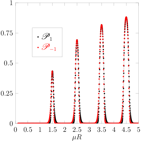
Figure 2 shows and as a function of . Each spike in and corresponds to a level transition in . Even though their behaviour as a function of is similar, the peaks of always preceed those of at the start and finish of each level transition.
Taking the temperature lower than that of Figure 2 causes the peaks to be narrower while maintaining the same height. Taking would make the peaks appear as infinitely narrow lines, occurring precisely at .
In Figure 3 we compare the first and fourth transitions. For non-zero , as increases the transition width, and thus the width of the deconfined regions, increases.
3.0.3 Pressure for
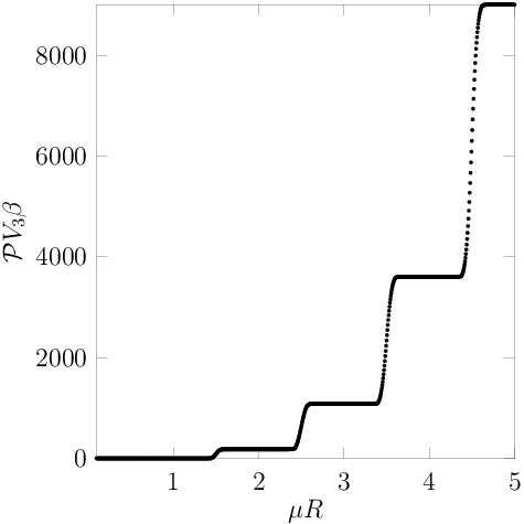

The pressure indicates how the system responds to changes in the spatial volume. The pressure multiplied by the 4-volume is shown in Figure 4 (Left) for . In the , limit the expectation value of the pressure is given by
| (46) |
which indicates that each level has a pressure
| (47) |
3.0.4 Energy for
The energy can be evaluated from the pressure and fermion number above and is plotted in Figure 4 (Right). The energy is calculated as
| (48) |
This shows that the energy levels are not horizontal. The factor of in front of the fermion number in the first line causes the levels to rise linearly with . The energy of each level is given by
| (49) |
3.0.5 Normalized , , for ; the Stefan-Boltzmann limit

The Stefan-Boltzmann limit is the zero interaction free fermion limit. On we obtain it from the one-loop result taking all the , corresponding to the deconfined phase, e.g., for the fermion number
| (50) |
The normalized fermion number, , is shown in Figure 5. The behavior of and as a function of is almost indistinguishable from . These results might at first seem at odds with the results for and , in the confined regions, since the are set to in , , and . The resolution is that sufficiently far within the confined regions the observables are independent of the . When is not close to for , then in the limit the terms drop out of the exponentials in the Fermi-Dirac distributions,
| (51) |
3.0.6 Average Phase for
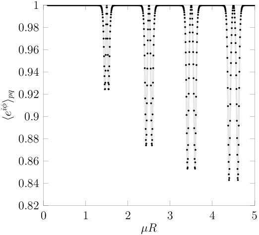
The average phase is important in that it shows where the sign problem is severe. It is given by
| (52) |
where the denominator is the “phase quenched” (real action) partition function,
| (53) |
Numerical results for the average phase are presented in Figure 6. The results suggest that the sign problem increases in severity with the chemical potential, then levels off (large results suggest it levels off near ). However, the average phase is only different from while and differ. This explains why the average phase is always in the middle of a transition. In fact, We observe that is smallest (largest) when is largest (smallest).
3.1 Chiral condensate
The chiral condensate is given by
| (54) |
In the massless limit as expected since it is a perturbative result, but it is interesting to note that in the light mass limit is linear in .
3.2 Continuum results ()
Since all of our observables are functions of the dimensionless quantities , , or , then we can obtain a “continuum” limit by taking one of the following:
- •
small (high temperature perturbation theory),
- •
large (high density perturbation theory),
- •
large (heavy quarks).
We take large to maintain validity in the region of the confinement-deconfinement transitions. For sufficiently large mass the fermion contribution to the action can be converted from a sum to an integral using the Abel-Plana formula and then simplified by taking . This proceeds as
| (55) |
The resulting integral formula removes all the periodic structure from the observables. It should be noted that this result is only valid in the vicinity of, . Once the chemical potential becomes sufficiently large compared to the fermion mass then the periodic structure returns and the system behaves again as it did in the massless case.
3.2.1 for


For QCD with non-zero quark mass the expectation values , , and exhibit “Silver Blaze” behavior: bulk observables are zero until onset [12] which occurs when the chemical potential reaches the value of the lightest quark mass. Here onset occurs for . The fermion number is given by
| (56) |
Each level has height
| (57) |
and level width
| (58) |
The Stefan-Boltzmann values shift accordingly as well, e.g., for the fermion number
| (59) |
The fermion number for large quark mass is plotted in Figure 7. The dots are calculated using the full sum form of (line of eq. (55)) and the green curves are from the integral approximation (line ). As expected is close to until the onset transition at . The smoothness of as it increases from onset results from the decreased level width in the large limit. It is only temporary though; as is increased further from the levels spread out and eventually the observables behave as they would for . This is reflected in the oscillations that develop as is increased when considering the full sum form of . The lack of these oscillations in the integral form shows that this approximation breaks down for values of away from the onset transition at . How long this breakdown takes depends on . The larger the , the further in we can go before breakdown.
3.2.2 Polyakov lines: and and average phase for


As in the discrete case, in the large limit the behavior of precedes that of as a function of . The transition in occurs around onset at and appears sharper for larger . Results for near the transition are presented in Figure 8 (Left), which shows and using the sum form of (black dots) and the integral approximation (green and blue curves). It is clear again that the integral approximation breaks down after the transition.
Figure 8 (Right) shows the average phase near the transition. After the transition, and before is sufficiently large that oscillations return full force, there is a brief respite from the sign problem in that the average phase is close to . The small spike in at corresponds to the value of where and differ maximally and serves as a good indicator of the location of the transition. Eventually, regardless of how large we make , the oscillations always return by taking sufficiently bigger.
4 The Large Theory at Low
In this section we turn to an analysis of the large- theory, specifically in the low-temperature limit . We showed in (26) that in this limit the system reduced to a unitary matrix model with a potential determined by the quarks.44 4 A similar matrix model but defined in the canonical ensemble and truncated so as to include only the term was considered in [34]. We work directly in the grand canonical ensemble and it is important in our analysis that we do not truncate the sum over in the fermionic sector.
Without the chemical potential, the potential in (26) would vanish in the low temperature limit. In this case, the Vandermonde piece dominates leading to a repulsion of the eigenvalues and so the integral is dominated by a uniform distribution of the angles around the circle. Consequently and the theory is in the confining phase. However, if as we simultaneously tune keeping fixed, where is one of the energy levels of the fermion system then the fermion term can compete with the van de Monde piece and a phase transition can occur. In fact this is a version of the Gross-Witten transition [29] (see also [30, 31]). The Gross-Witten transition is typically a third order phase transition that occurs in large gauge theories in finite volume and involves a transition from a configuration where the density of eigenvalues of the Polyakov line lies on the unit circle in the complex plane to a configuration with a gap. We loosely refer to this as a confinement/deconfinement transition because the confined phase defined by a distribution that lies on a closed contour is smoothly connected to the phase where the eigenvalues are uniformly distributed around the unit circle and , for , indicative that it costs an infinite amount of energy to propagate colour charges. Correspondingly the deconfined phase defined by a distribution that has a gap is smoothly connected to the configurations where all the eigenvalues , i.e. where colour charges are free to propagate indicative of a plasma phase. We will find that, as suggested by the results, increasing the chemical potential induces a series of such transitions, the novel aspect being that the eigenvalues no longer lie on the unit circle due to the complex action.
Without-loss-of-generality we will choose to be positive so that only the contribution from the quarks survive and the quark potential takes the form
| (60) |
Notice that the potential is not hermitian. This is the usual “sign problem” in the presence of a chemical potential. In the context of the matrix model, it means that the saddle point that dominates in the large limit will lie at complex angles . In this respect the matrix model is of the “holomorphic” type that appears in the Dijkgraaf-Vafa approach to supersymmetric gauge theories and in particular [35] which considered the unitary version.
4.1 Single level model
For the moment let us focus on what can happen with a single level and . Defining an effective fugacity the effective action on the angles, including the Vandermonde piece, is
| (61) |
where we have added the Lagrange multiplier to enforce the constraint, i.e. .
In the large limit, the integral over the angles is dominated by a saddle point obtained by solving the equation-of-motion that follows from (61)
| (62) |
As we remarked above, our system is a unitary matrix model with a non-standard kind of potential term coming from the fermions. What is novel in the present context is that the potential is not real and as a consequence the saddle-point configuration will lie out in the complex plane. In fact if we define then in the presence of the non-real potential the will move off the unit circle in the -plane. As a consequence if we define the observables
| (63) |
we will find that on the saddle point solution.
Before we plunge in and solve the matrix model, it is useful to note that when is either very small or large, the potential vanishes (in the latter case following from using the constraint ) and so we expect the to be uniformly distributed around the unit circle. Taking the equation-of-motion in terms of the variables
| (64) |
it then follows that as the Lagrange multiplier while as the Lagrange multiplier . The Lagrange multiplier has an important interpretation following from (64):
| (65) |
and so is the effective fermion number, . So as varies from to the picture is that the energy level becomes occupied and the effective fermion number jumps by the factor . The question before us is to establish how this transition occurs.
The small confined phase
We make the hypothesis that as increases from 0 that the eigenvalues are continuously distributed around a closed contour in the -plane at least up to some finite value of . In the large limit, we can describe the distribution of eigenvalues by an analytic function for which along is real and positive. It is useful to think of in terms of a conformal map of the cylinder , , , for which the eigenvalues are uniformly distributed along the real axis between and , to the -plane:
| (66) |
where the contour is obtained from the inverse map obtained by solving the differential equation
| (67) |
subject to the initial condition that when we have . For consistency we must also have so that is closed. The normalization condition is
| (68) |
where the left-hand side can be evaluated using Cauchy’s theorem. The condition, , translates into the constraint
| (69) |
where the branch cut of the logarithm is taken through the contour at the point .
In the large- limit the saddle-point equation (64) becomes for
| (70) |
The here indicates a principal value which is the required prescription given that lies on integration contour . In practical terms this means that the right-hand side is the average of two terms with infinitesimally just inside and just outside the integration contour. The right-hand side can then be evaluated by Cauchy’s theorem yielding an expression of the form where the ellipsis represent other terms that arise when has other poles inside . It is clear that can only have poles at and . The condition (68) implies that the pole at must be inside and have unit residue. The only question is whether the pole at is inside or not. In the small region, it will be outside—indeed this will define the small region. Consequently, from (65)
| (71) |
The form of is then completely fixed by (70) to be
| (72) |
One can check that the constraint (69) is satisfied. Notice that as , , which is the uniform distribution around the unit circle. The contour follows by solving (67) for to give
| (73) |
and then inverting to give . Notice that the integration constant is fixed by requiring that as we have (the uniform distribution of eigenvalues). In this small confining phase the effective fermion number vanishes and the Polyakov line expectation values are
| (74) |
As advertised, as a symptom of having a complex action, .
The question is what happens to this phase as increases. The issue is that the pole of at must lie outside , however, this cannot be maintained when becomes large enough. To see what happens notice that vanishes at , a point that lies outside for small . As increases to the value
| (75) |
vanishes precisely on at the point on the negative real axis. At this point develops a kink and beyond this value of the inverse solution to (73) ceases to be closed . This signals that a phase transition will occur to a configuration where the contour opens into an arc, just as in the matrix model solved by Gross and Witten [29]. The line of the phase transitions in the plane corresponds to the straight line
| (76) |
valid in the low temperature limit.
The large confined phase
We can solve for the large phase in a similar way. In this case the pole of at is now inside . The solution turns out to be
| (77) |
which satisfies (70) and (68) with . In addition, one can check that the constraint (69) is satisfied. Notice that as , we have , as required. The contour follows by solving (67) to get
| (78) |
In this phase the effective fermion number —the level is now occupied—and the Polyakov line expectation values are
| (79) |
So comparing with (74), the behaviour of swaps over along with the replacement .
As in the small phase, the large phase persists until the zero of , at which lies inside for large enough , just touches . This occurs when
| (80) |
For smaller values of , the contour is not closed and the phase does not exist. Notice that the points of transition and satisfy . In the plane the boundary lies along the straight line
| (81) |
valid in the low temperature limit.
The deconfined phase
In the region , experience with the Gross-Witten matrix model suggests that the eigenvalues lie on an open contour . In this case, the model can be solved by the standard resolvant/spectral curve method. The resolvant is defined as the function
| (82) |
By hypothesis, in the large limit the eigenvalues distribute themselves on an open contour and is a function which is analytic everywhere in the -plane except along a square-root branch cut running along with branch points, and , lying at the endpoints, as illustrated in Figure 9. The eigenvalues are then distributed along the cut between the branch points, such that
| (83) |
it follows from this representation that as and
| (84) |
From the Plemelj formulae [36], the equation-of-motion (70) is simply the condition
| (85) |
where is an infinitesimal such that lies on either side of the cut.55 5 This is a definition of the principal value in (70). It follows from (83) and the Plemelj formulae that the density of eigenvalues is obtained as the discontinuity of across the cut :
| (86) |
In particular, this means that an average of the form
| (87) |
can be used where is a contour which encircles as illustrated in Figure 9. This can then be evaluated by pulling the closed contour off the cut to pick up the residues in the -plane.

The resolvant can be written down based on the following conditions: it is an analytic function in the -plane apart from a single square-root branch cut, it satisfies the conditions (84), and . The solution to the equation-of-motion (85) is of the form
| (88) |
The endpoints , and the function are then determined by imposing (84) and requiring that is regular at . These conditions uniquely determine
| (89) |
and the endpoints of are given by
| (90) |
What remains is to fix by imposing the final condition (69) which becomes
| (91) |
Pulling the contour off the cut, deforming it around the poles at and collecting their residues, and adding the discontinuity from the branch cut of gives66 6 For another example see [37].
| (92) |
where and are cut-offs and the integrals around and are defined on the contours and , , respectively. The limit is well defined since the factors of and separately cancel. What remains is the condition
| (93) |
This equation determines as a function of . An important check on the solution is how the deconfined phase interfaces with the small and large closed phases. When we have and at this point and so the two branch points come together and one can readily verify that the density matches that of the small phase at the edge of its existence at . The same happens at when where the gapped phase merges continuously with the large closed phase.
From (93) it follows that across the transitions at and , and its first derivative are continuous, however higher derivatives are discontinuous. Since is the effective fermion number, the first derivative of the grand potential, it follows that the transitions are third order just as in the original Gross-Witten model [29]. The behaviour of the effective fermion number as is increased past is shown in Figure 10.

The expectation values of the Polyakov line in the deconfined phase can be determined from an expansion of the resolvant for and [38],
| (94) |
| (95) |
where is the number of windings. For a single winding, the Polyakov lines are
| (96) |
where via the inversion of (93) and . The behaviour of is shown in Figure 11. Notice how vanish in the small and large confined phases, respectively.
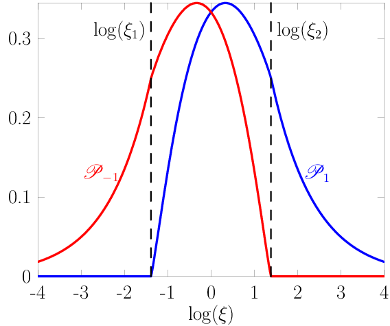
The behaviour of the contour is shown in the three plots that make up Figure 12. These plots also show how the pole at is “eaten” as one goes from the small to large phases. Finally Figure 13 shows schematically the phase diagram in the plane in the vicinity of and at low temperature.


4.2 Multi-level model
In the full QCD model there are, of course a series of energy levels as in (60). For a series of levels we can write
| (97) |
with
| (98) |
In general a matrix model with such a potential could exhibit a rich set of phases where the eigenvalues have support over a multiple set of open contours, the “multi-cut” solutions. These multi-cut solutions arise when the potential has multiple degenerate minima and the cuts are located around the minima. In the present case the potential apparently does not exhibit multiple minima and so we suspect that these multi-cut solutions never dominate the ensemble. Henceforth, we will only consider solutions with a closed contour, the confining phase, and with single cuts, the deconfined phase, leaving a detailed analysis of multi-cut solutions for the future.
When is low enough, experience with the single-level model suggests that as increases the system goes through a series of phase transitions with a confined phase lying in a window of with , for which the closed contour contains the poles , with . In this case the saddle-point equation is solved by
| (99) |
with the effective fermion number
| (100) |
indicating the first levels are filled.
The actual distribution of eigenvalues follows from integrating (67) which gives
| (101) |
The phase only exists over the finite region of for which so that the contour is actually closed. The boundary of this region can be obtained by the condition that on the boundary at some point on . This defines a triangular shaped region in the plane which at covers the region . The apex of the triangle lies at a special point where has a double zero on . So with a number of energy levels the boundary of the confined phases describes a saw-tooth pattern in the plane as illustrated in Figure 14.

4.3 The continuum model
In the limit, , the fermionic levels form an approximate continuum starting at and extending up to roughly where the discrete structure starts to manifest itself again. As long as the temperature is not too low, (along with required to have a unitarity matrix model) the sum over levels can be approximated by a continuum of the form
| (102) |
where and , with . In this case,
| (103) |
Based on what we have learnt hitherto, we expect that in this case there is a confined phase for small enough and then a transition to a deconfined phase at . In this case for larger the deconfined phase persists since the cut in (103) does not allow the end-points of the open distribution to close up again. So the validity of the continuum approximation implies a which is large enough so that there is no series of transitions. The confined phase is simple to analyse using the techniques in earlier sections. One finds that and the density is
| (104) |
The contour is determined by inverting
| (105) |
The phase persists up to a value of such that the zero of at, say ( and ), lies on the contour , which means that and are roots of
| (106) |
Since , the solution is approximately and and so the transition occurs at
| (107) |
The deconfined phase in this case is described by a resolvent
| (108) |
In principle, one can find numerically, however, we don’t pursue this analysis here.
5 The Large Theory in the Plane
When we move out of the regime of low temperature, so that is no longer , into the whole plane, the factors in (21) cannot be ignored. Hence, the measure on can no longer be approximated by that of a unitary matrix. In this case, we can in principle solve the model in the confining phase, where the eigenvalues lie on a closed contour by introducing the Laurent expansion
| (109) |
where follows from the normalization condition. In terms of the components, the action of the Polyakov line with fundamental fermions is
| (110) |
The action is quadratic in the and so the saddle-point is easily found to be at
| (111) |
for and . Note that the condition (69) is automatically satisfied. The boundary of the confining phase is then obtained by solving for the condition that for lying on the contour which itself is determined from (67).
When , and in the intermediate regime
| (112) |
we have already determined that there is a Gross-Witten transition (107). At we know that, for , the fermionic modes are decoupled. So we have effectively the pure gauge theory which is known to have a confinement/deconfinement transition driven by the modes at a temperature where , giving [3]. This transition is known to be first order even when higher order corrections in the coupling are considered; in fact the first correction to the Gaussian approximation requires a 3-loop computation [39]. For finite fermion mass the transition occurs below . If we make the approximation of ignoring the higher modes , , then the transition happens when such that
| (113) |
and is a third order Gross-Witten transition. The case with was considered in [40].
The Gross-Witten transition at extends out into the plane and joins smoothly with the transition line that comes from the first energy level. Although the line of transitions can be determined numerically a good approximation is obtained by keeping only the first 2 modes . A schematic picture of the phase diagram for the large mass regime is shown in Figure 15. We have also indicated on this diagram the discrete sawtooth structure which can be seen at very low temperatures . In this regime the peaks rise until approaches and then they decrease slowly.

When is reduced, the transition at occurs at a lower temperature and a schematic picture of the phase diagram appears in Figure 16. Now the sawtooth structure extends all the way to small .

6 Comparison of and


It is meaningful to compare the results we have obtained using the two different calculational techniques presented in this paper. This is useful not only towards checking our results, but also towards learning about what differences might arise when considering small vs. large , and under which conditions there is agreement.
We consider a single level transition, , and , which is the value used in the calculations. In Figure 17 (Left) we show an overlay of the and results for the fermion number normalized by . The transitions between the small confined phase and the deconfined phase, and also between the deconfined phase and the large confined phase, are clearly signified by discontinuities for , but they are smoothed out for . Taking lower temperatures does not sharpen the result since we are plotting as a function of rather than . It may be that the transitions are smoother for as a result of working in a small spatial volume. The important feature of this comparison is that the calculation suggests possible transitions and the calculation confirms them.
In Figure 17 (Right) we show the Polyakov lines and for and . Again the discontinuities which occur at the transitions in the case are lost for . In addition, since the difference , and given our observation that the severity of the sign problem increases with , then it appears that the sign problem would always be more severe in the large limit.


It is also possible to solve for the distribution from the expectation values of the angles of the Polyakov line for , for the purpose of comparing with . To do this we solve the characteristic equation
| (114) |
This result can be expanded and rewritten in terms of the expectation values , and , determined earlier, to give
| (115) |
We find the three solutions for (using our results for and at the level transition) for four different values of in each of the regions , , and . The results are given by the points in Figure 18. The contours are interpolations of the points and give a rough idea of how the distribution changes with . Comparing with the large results for the distribution, given in Figure 12, we see that the direction of movement of the distribution matches up in all three regions: In the complex -plane, for the contour passes from the unit circle to the left with increasing , for it passes back to the right passing by the unit circle, and for the distribution moves left again back to the unit circle.
It is also worth noting that there is agreement between the large finite temperature phase diagrams in Figures 15 and 16, and the low temperature results for the Polyakov line for in Figures 2, and 8 (Left). In the case of a massless quark, and at low temperatures, we see a widening of the deconfined phases for increasing . For a massive quark, at low but non-zero temperature, there is a brief respite from the oscillating phases after the onset transition to the first deconfined phase at , but taking large enough causes the oscillations to return.
7 Conclusions and Outlook
We have performed a one-loop analytical derivation of the phase diagram of QCD as a function of temperature and chemical potential, in the large and limit, on , and supported the low temperature results with numerical calculations for . In the case of massless quarks, and considering the low temperature limit, we observe a series of confinement-deconfinement transitions as a function of the chemical potential. In the large limit the phases are characterized by the distribution of the Polyakov line eigenvalues in the complex plane which can be obtained using matrix model techniques that have been generalized for a complex action. In the large quark mass limit we observe the “Silver Blaze” feature in that bulk observables are roughly zero until the onset transition to the deconfined phase which occurs at . From here there is a brief continuum-like behavior in that the observables appear smooth after the transition. This behavior continues until is sufficiently larger than that the levels spread out and the confinement-deconfinement phase oscillations return.
From a physical standpoint, a remarkable aspect of our results is the correlation between deconfinement and the existence of partially filled quark shells in a box. From the behaviour of the fermion number at low temperatures we observe that each confinement-deconfinement transition in the Polyakov line is associated with a level transition. All energy levels below the Fermi energy, given by the chemical potential, are filled, and levels above the Fermi energy are empty. There are clear analogies with partially-filled bands in condensed matter physics; here we would say that the Fermi energy in such a system falls within a band, resulting in a conducting ground state. A more accurate analogy, since it involves a finite number of particles, would be partially-filled shells in nuclear physics. The lesson we draw is that de-confinement appears to require a non-zero density of gapless states. We also learn that these states are either particle-like or hole-like depending on which edge of the band is closer. Because particles and holes carry conjugate representations of the gauge group the resulting physics is distinct, as revealed by the differing behaviours of and . The non-monotonic behaviour of has been observed in lattice simulations of QCD with gauge group SU(2) near its saturation density (i.e. quarks per lattice site) [20].
There are a number of interesting generalizations that might be made. One could consider more quark flavours with different masses , perhaps coupled to different chemical potentials . A detailed multidimensional phase diagram could be calculated as a function of the quark masses and their chemical potentials. There may be a sign of color superconducting phases from the configurations of the gauge field. It might be interesting to consider different manifolds as well. In addition, a numerical computation of the line of transitions in the plane can be performed from the results for the large calculation to connect the transition points on the and axes for large quark mass, and the curvature of this line can be determined. In the event that lattice simulations of QCD become possible at moderate chemical potential in the low temperature limit, it would be interesting to see if the low temperature confinement-deconfinement phase oscillations we have observed as a function of are present at strong coupling and/or large volume. We are currently investigating this possibility in simulations of QCD with .
Our analysis has been limited to the Gaussian approximation and it is clearly important to consider systematically the effect of higher orders in the gauge coupling. This kind of higher order analysis was qualitatively undertaken in the thermal theory in [3]. It turns out that in this case the fate of the confinement/deconfinement transition depends critically on the sign of the coefficient of a 3-loop term in the expansion of the effective action. Whilst this 3-loop calculation has not been performed for the gauge theory it has for the pure gauge theory in [39]. This tour de force calculation proves that the transition survives as a first order transition. The effect of higher orders in the coupling for the theory with fundamental flavours (with have been considered qualitatively in [41, 42]. This latter work suggests in the theory with that the confinement/deconfinement transition disappears and becomes a cross-over as is increased beyond a certain critical value. It will be interesting to see how this is altered in the presence of a chemical potential. It will be interesting to see whether the phase structure that we find can be related to that of a theory with an AdS/CFT-type gravity dual. For instance, will the infinite sequence of Gross-Witten transitions that we see be seen in the dual gravitational description?
8 Acknowledgements
We would like to thank Gert Aarts, Prem Kumar, and Rob Pisarski for useful discussions.
References
- [1] E. Witten, Adv. Theor. Math. Phys. 2 (1998) 505 [arXiv:hep-th/9803131].
- [2] B. Sundborg, Nucl. Phys. B 573 (2000) 349 [arXiv:hep-th/9908001].
- [3] O. Aharony, J. Marsano, S. Minwalla, K. Papadodimas and M. Van Raamsdonk, Adv. Theor. Math. Phys. 8, 603 (2004) [arXiv:hep-th/0310285].
- [4] D. Yamada and L. G. Yaffe, JHEP 0609 (2006) 027 [arXiv:hep-th/0602074].
- [5] G. Veneziano, Nucl. Phys. B 117 (1976) 519.
- [6] A. Karch and A. O’Bannon, Phys. Rev. D 74 (2006) 085033 [arXiv:hep-th/0605120].
- [7] A. Karch, A. O’Bannon and L. G. Yaffe, JHEP 0909 (2009) 042 [arXiv:0906.4959 [hep-th]].
- [8] A. M. Halasz, A. D. Jackson, R. E. Shrock, M. A. Stephanov and J. J. M. Verbaarschot, Phys. Rev. D 58 (1998) 096007 [arXiv:hep-ph/9804290].
- [9] M. G. Alford, A. Schmitt, K. Rajagopal and T. Schafer, Rev. Mod. Phys. 80 (2008) 1455 [arXiv:0709.4635 [hep-ph]].
- [10] A. Kurkela, P. Romatschke and A. Vuorinen, arXiv:0912.1856 [hep-ph].
- [11] S. Hands, Prog. Theor. Phys. Suppl. 168 (2007) 253 [arXiv:hep-lat/0703017].
- [12] T. D. Cohen, Phys. Rev. Lett. 91 (2003) 222001 [arXiv:hep-ph/0307089].
- [13]
J. C. Osborn,
Phys. Rev. Lett. 93 (2004) 222001
[arXiv:hep-th/0403131];
G. Akemann, J. C. Osborn, K. Splittorff and J. J. M. Verbaarschot, Nucl. Phys. B 712 (2005) 287 [arXiv:hep-th/0411030];
J. C. Osborn, K. Splittorff and J. J. M. Verbaarschot, Phys. Rev. Lett. 94 (2005) 202001 [arXiv:hep-th/0501210]. - [14] Z. Fodor and S. D. Katz, JHEP 0203 (2002) 014 [arXiv:hep-lat/0106002]; JHEP 0404 (2004) 050 [arXiv:hep-lat/0402006].
- [15] C. R. Allton et al., Phys. Rev. D 66 (2002) 074507 [arXiv:hep-lat/0204010]; Phys. Rev. D 68 (2003) 014507 [arXiv:hep-lat/0305007].
- [16]
P. de Forcrand and O. Philipsen,
Nucl. Phys. B 642 (2002) 290
[arXiv:hep-lat/0205016];
M. D’Elia and M. P. Lombardo, Phys. Rev. D 67 (2003) 014505 [arXiv:hep-lat/0209146]. - [17] D. T. Son and M. A. Stephanov, Phys. Rev. Lett. 86 (2001) 592 [arXiv:hep-ph/0005225].
- [18] J. B. Kogut, M. A. Stephanov, D. Toublan, J. J. M. Verbaarschot and A. Zhitnitsky, Nucl. Phys. B 582 (2000) 477 [arXiv:hep-ph/0001171].
- [19]
S. Hands, I. Montvay, S. Morrison, M. Oevers, L. Scorzato and J. Skullerud,
Eur. Phys. J. C 17 (2000) 285
[arXiv:hep-lat/0006018];
R. Aloisio, V. Azcoiti, G. Di Carlo, A. Galante and A. F. Grillo, Phys. Lett. B 493 (2000) 189 [arXiv:hep-lat/0009034];
J. B. Kogut, D. K. Sinclair, S. J. Hands and S. E. Morrison, Phys. Rev. D 64 (2001) 094505 [arXiv:hep-lat/0105026]. - [20] S. Hands, S. Kim and J. I. Skullerud, Eur. Phys. J. C 48 (2006) 193 [arXiv:hep-lat/0604004]; arXiv:1001.1682.
- [21] O. Aharony, K. Peeters, J. Sonnenschein and M. Zamaklar, JHEP 0802 (2008) 071 [arXiv:0709.3948 [hep-th]].
- [22] M. G. Endres, Phys. Rev. D 75 (2007) 065012 [arXiv:hep-lat/0610029].
- [23] D. Banerjee and S. Chandrasekharan, arXiv:1001.3648.
- [24] P. de Forcrand and M. Fromm, Phys. Rev. Lett. 104 (2010) 112005 [arXiv:0907.1915 [hep-lat]].
- [25] G. Aarts and I. O. Stamatescu, JHEP 0809 (2008) 018 [arXiv:0807.1597 [hep-lat]].
- [26]
G. Aarts,
Phys. Rev. Lett. 102 (2009) 131601
[arXiv:0810.2089 [hep-lat]];
G. Aarts, F. A. James, E. Seiler and I. O. Stamatescu, arXiv:0912.0617. - [27] D. Persson and V. Zeitlin, Phys. Rev. D 51 (1995) 2026 [arXiv:hep-ph/9404216].
- [28] V. Zeitlin, Phys. Lett. B 352 (1995) 422 [arXiv:hep-th/9410064].
- [29] D. J. Gross and E. Witten, Phys. Rev. D 21 (1980) 446.
- [30] S. Wadia, “A Study Of U(N) Lattice Gauge Theory In Two-Dimensions,” EFI-79/44-CHICAGO.
- [31] S. R. Wadia, Phys. Lett. B 93, 403 (1980).
- [32] D. J. Gross, R. D. Pisarski and L. G. Yaffe, Rev. Mod. Phys. 53 (1981) 43.
- [33] A. Dumitru, R. D. Pisarski and D. Zschiesche, Phys. Rev. D 72 (2005) 065008 [arXiv:hep-ph/0505256].
- [34] S. I. Azakov, P. Salomonson and B. S. Skagerstam, Phys. Rev. D 36 (1987) 2137.
- [35] R. Dijkgraaf and C. Vafa, Nucl. Phys. B 644, 21 (2002) [arXiv:hep-th/0207106].
- [36] N. I. Muskhelishvili, Singular Integral Equations: Boundary Problems of Function Theory and Their Application to Mathematical Physics, Dover, New York, 2008.
- [37] X. Arsiwalla, R. Boels, M. Marino and A. Sinkovics, Phys. Rev. D 73 (2006) 026005 [arXiv:hep-th/0509002].
- [38] G. W. Semenoff, arXiv:hep-th/0405107.
- [39] O. Aharony, J. Marsano, S. Minwalla, K. Papadodimas and M. Van Raamsdonk, Phys. Rev. D 71 (2005) 125018 [arXiv:hep-th/0502149].
- [40] H. J. Schnitzer, Nucl. Phys. B 695 (2004) 267 [arXiv:hep-th/0402219].
- [41] H. J. Schnitzer, arXiv:hep-th/0612099.
- [42] P. Basu and A. Mukherjee, Phys. Rev. D 78 (2008) 045012 [arXiv:0803.1880 [hep-th]].