Lattice calculations for $A=3,4,6,12$ nuclei
using chiral effective field theory

Evgeny Epelbaum^a, Hermann Krebs^a, Dean Lee^b,c, Ulf-G. Meißner^c,d,e Affiliation: ^aInstitut für Theoretische Physik II, Ruhr-Universität Bochum, D-44780 Bochum, Germany ^bDepartment of Physics, North Carolina State University, Raleigh, NC 27695, USA ^cHelmholtz-Institut für Strahlen- und Kernphysik (Theorie) and Bethe Center for Theoretical Physics, Universität Bonn, D-53115 Bonn, Germany ^dInstitut für Kernphysik (IKP-3) and Jülich Center for Hadron Physics, Forschungszentrum Jülich, D-52425 Jülich, Germany ^eInstitute for Advanced Simulation (IAS-4), Forschungszentrum Jülich, D-52425 Jülich, Germany

Abstract

We present lattice calculations for the ground state energies of tritium, helium-3, helium-4, lithium-6, and carbon-12 nuclei. Our results were previously summarized in a letter publication. This paper provides full details of the calculations. We include isospin-breaking, Coulomb effects, and interactions up to next-to-next-to-leading order in chiral effective field theory.

pacs

21.10.Dr, 21.30.-x, 21.45-v, 21.60.De

I Introduction

Lattice effective field theory combines the theoretical framework of effective field theory with numerical lattice methods. In contrast with most other ab initio methods, systematic errors are all introduced at the beginning when defining the truncated low-energy effective theory. The errors can be clearly identified as either missing operators in the lattice action, finite volume effects, or errors from finite Euclidean-time extrapolation. Future studies can build upon existing calculations in a straightforward manner by including the missing operators, increasing the volume, or improving the Euclidean-time extrapolation.

Lattice effective field theory has been used to study nuclear matter [1] and neutron matter [2, 3, 4, 5, 6, 7]. The method has also been applied to nuclei with $A\leq 4$ using effective field theory with and without pions [8, 9, 10]. A review of lattice effective field theory calculations can be found in Ref. [11]. Reviews of chiral effective field theory can be found in Ref. [12, 13, 14, 15].

In this paper we present the first lattice results for lithium-6 and carbon-12 using chiral effective field theory. We also present the first lattice calculations to include isospin-breaking and Coulomb effects. Our results were previously summarized in a letter publication [16]. This paper provides full details of the calculations. We begin by describing the lattice interactions in chiral effective field theory appearing at leading order, next-to-leading order, and next-to-next-to-leading order. This is followed by a discussion of isospin-breaking and Coulomb interactions. After this all unknown operator coefficients are fit using low-energy scattering data. We then compute the energy splitting between the triton and helium-3. We discuss the auxiliary-field Monte Carlo projection method and an approximate universality of contributions from higher-order interactions in systems with four or more nucleons. This is followed by lattice results for the ground state energy of helium-4, lithium-6, and carbon-12.

II Leading order

The low-energy expansion in effective field theory counts powers of the ratio $Q$ / $\Lambda$ . $\ Q$ is the momentum scale associated with the mass of the pion or external nucleon momenta, and $\Lambda$ is the momentum scale at which the effective theory breaks down. At leading order (LO) in the Weinberg power-counting scheme [17, 18], the nucleon-nucleon effective potential contains two independent contact interactions and instantaneous one-pion exchange. As in previous lattice studies we make use of an “improved” leading-order action. This improved leading-order action is treated completely non-perturbatively, while higher-order interactions are included as a perturbative expansion in powers of $Q/\Lambda$ .

In our lattice calculations we use the improved LO₃ lattice action introduced in Ref. [6] with spatial lattice spacing $a=(100$ MeV $)^{-1}=1.97$ fm and temporal lattice spacing $a_{t}=(150$ MeV $)^{-1}=1.32$ fm. We take the parameter values $g_{A}=1.29$ , $\ f_{\pi}=92.2$ MeV, $m_{\pi}=m_{\pi^{0}}=134.98$ MeV. For the nucleon mass we use $m=938.92$ MeV. Many of the calculations presented in this paper have never been attempted before, and our choice of spatial lattice spacing is made to optimize the efficiency of the Monte Carlo lattice calculations. While $1.97$ fm is much larger than lattice spacings used lattice QCD simulations, we should emphasize that we are not probing the quark and gluon substructure of nucleons but rather the distribution of nucleons within nuclei. Our lattice spacing corresponds with a maximum filling density of more than three times normal nuclear matter density. In future studies the same systems will also be analyzed using smaller lattice spacings.

Throughout this discussion we first present the interactions in continuum notation and then later give the corresponding lattice operator. For the continuum notation we give matrix elements for incoming and outgoing two-nucleon momentum states. In the following $\vec{q}$ denotes the $t$ -channel momentum transfer. We use $\boldsymbol{\tau}$ to represent Pauli matrices in isospin space and $\vec{\sigma}$ for Pauli matrices in spin space. The interactions correspond with the amplitude,

$\displaystyle\mathcal{A}\left(V_{\text{LO}}\right)$	$\displaystyle=C_{S=0,I=1}f(\vec{q})\left(\frac{1}{4}-\frac{1}{4}\vec{\sigma}_{A}\cdot\vec{\sigma}_{B}\right)\left(\frac{3}{4}+\frac{1}{4}\boldsymbol{\tau}_{A}\cdot\boldsymbol{\tau}_{B}\right)$
	$\displaystyle+C_{S=1,I=0}f(\vec{q})\left(\frac{3}{4}+\frac{1}{4}\vec{\sigma}_{A}\cdot\vec{\sigma}_{B}\right)\left(\frac{1}{4}-\frac{1}{4}\boldsymbol{\tau}_{A}\cdot\boldsymbol{\tau}_{B}\right)$
	$\displaystyle-\left(\frac{g_{A}}{2f_{\pi}}\right)^{2}\frac{\left(\boldsymbol{\tau}_{A}\cdot\boldsymbol{\tau}_{B}\right)\left(\vec{q}\cdot\vec{\sigma}_{A}\right)\left(\vec{q}\cdot\vec{\sigma}_{B}\right)}{q^{2}+m_{\pi}^{2}}.$	(1)

We use a Euclidean-time transfer-matrix lattice formalism. The transfer matrix is the normal-ordered exponential of the lattice Hamiltonian, $\colon\exp(-H\Delta t)\colon$ , where $\Delta t$ equals one temporal lattice spacing. We use the lattice notation adopted in several previous publications and which is summarized in the appendix. Let $V_{S=0,I=1}$ be the lattice density-density correlation for the spin-singlet isospin-triplet channel in momentum space,

	$\displaystyle V_{S=0,I=1}(\vec{q})$	$\displaystyle=\frac{3}{32}:\rho^{a^{{\dagger}},a}(\vec{q})\rho^{a^{{\dagger}},a}(-\vec{q}):-\frac{3}{32}:\sum_{S}\rho_{S}^{a^{{\dagger}},a}(\vec{q})\rho_{S}^{a^{{\dagger}},a}(-\vec{q}):$
		$\displaystyle+\frac{1}{32}:\sum_{I}\rho_{I}^{a^{{\dagger}},a}(\vec{q})\rho_{I}^{a^{{\dagger}},a}(-\vec{q}):-\frac{1}{32}:\sum_{S,I}\rho_{S,I}^{a^{{\dagger}},a}(\vec{q})\rho_{S,I}^{a^{{\dagger}},a}(-\vec{q}):.$		(2)

Let $V_{S=1,I=0}$ be the density-density correlation for the spin-triplet isospin-singlet channel,

	$\displaystyle V_{S=1,I=0}(\vec{q})$	$\displaystyle=\frac{3}{32}:\rho^{a^{{\dagger}},a}(\vec{q})\rho^{a^{{\dagger}},a}(-\vec{q}):+\frac{1}{32}:\sum_{S}\rho_{S}^{a^{{\dagger}},a}(\vec{q})\rho_{S}^{a^{{\dagger}},a}(-\vec{q}):$
		$\displaystyle-\frac{3}{32}:\sum_{I}\rho_{I}^{a^{{\dagger}},a}(\vec{q})\rho_{I}^{a^{{\dagger}},a}(-\vec{q}):-\frac{1}{32}:\sum_{S,I}\rho_{S,I}^{a^{{\dagger}},a}(\vec{q})\rho_{S,I}^{a^{{\dagger}},a}(-\vec{q}):.$		(3)

We use these functions to write the leading-order transfer matrix,

	$\displaystyle M_{\text{LO}}$	$\displaystyle=\colon\exp\left\{-H_{\text{free}}\alpha_{t}-\frac{\alpha_{t}}{L^{3}}\sum_{\vec{q}}f(\vec{q})\left[C_{S=0,I=1}V_{S=0,I=1}(\vec{q})+C_{S=1,I=0}V_{S=1,I=0}(\vec{q})\right]\right.$
		$\displaystyle\qquad+\left.\frac{g_{A}^{2}\alpha_{t}^{2}}{8f_{\pi}^{2}q_{\pi}}\sum_{\begin{subarray}{c}S_{1},S_{2},I\end{subarray}}\sum_{\vec{n}_{1},\vec{n}_{2}}G_{S_{1}S_{2}}(\vec{n}_{1}-\vec{n}_{2})\rho_{S_{1},I}^{a^{{\dagger}},a}(\vec{n}_{1})\rho_{S_{2},I}^{a^{{\dagger}},a}(\vec{n}_{2})\right\}\colon.$		(4)

The momentum-dependent coefficient function $f(\vec{q})$ is given by

f(\vec{q})=f_{0}^{-1}\exp\left[-b{\displaystyle\sum\limits_{l}}\left(1-\cos q_{l}\right)\right],

(5)

where

f_{0}=\frac{1}{L^{3}}\sum_{\vec{q}}\exp\left[-b{\displaystyle\sum\limits_{l}}\left(1-\cos q_{l}\right)\right].

(6)

We use the value $b=0.6$ , which gives approximately the correct effective range for the two $S$ -wave channels when $C_{S=0,I=1}$ and $C_{S=1,I=0}$ are tuned to the physical $S$ -wave scattering lengths.

III Next-to-leading order

At next-to-leading order (NLO) the two-nucleon effective potential includes seven contact interactions carrying two powers of momentum, corrections to the two LO contact interactions, and the leading contribution from the instantaneous two-pion exchange potential (TPEP) [19, 20, 21, 22, 23],

V_{\text{NLO}}=V_{\text{LO}}+\Delta V^{(0)}+V^{(2)}+V_{\text{NLO}}^{\text{TPEP}}.

(7)

The tree-level amplitudes for the contact interactions are

\mathcal{A}\left(\Delta V^{(0)}\right)=\Delta C+\Delta C_{I^{2}}\boldsymbol{\tau}_{A}\cdot\boldsymbol{\tau}_{B}

(8)

and

$\displaystyle\mathcal{A}\left(V^{(2)}\right)$	$\displaystyle=C_{1}q^{2}+C_{2}k^{2}+\left(C_{3}q^{2}+C_{4}k^{2}\right)\left(\vec{\sigma}_{A}\cdot\vec{\sigma}_{B}\right)$
	$\displaystyle+iC_{5}\frac{1}{2}\left(\vec{\sigma}_{A}+\vec{\sigma}_{B}\right)\cdot\left(\vec{q}\times\vec{k}\right)$
	$\displaystyle+C_{6}\left(\vec{q}\cdot\vec{\sigma}_{A}\right)\left(\vec{q}\cdot\vec{\sigma}_{B}\right)+C_{7}\left(\vec{\sigma}_{A}\cdot\vec{k}\right)\left(\vec{\sigma}_{B}\cdot\vec{k}\right).$	(9)

The amplitude for the NLO two-pion exchange potential is [24, 25]

	$\displaystyle\mathcal{A}\left[V_{\text{NLO}}^{\text{TPEP}}\right]$	$\displaystyle=-\frac{\boldsymbol{\tau}_{A}\cdot\boldsymbol{\tau}_{B}}{384\pi^{2}f_{\pi}^{4}}L(q)\left[4m_{\pi}^{2}\left(5g_{A}^{4}-4g_{A}^{2}-1\right)+q^{2}\left(23g_{A}^{4}-10g_{A}^{2}-1\right)+\frac{48g_{A}^{4}m_{\pi}^{4}}{4m_{\pi}^{2}+q^{2}}\right]$
		$\displaystyle-\frac{3g_{A}^{4}}{64\pi^{2}f_{\pi}^{4}}L(q)\left[\left(\vec{q}\cdot\vec{\sigma}_{A}\right)\left(\vec{q}\cdot\vec{\sigma}_{B}\right)-q^{2}\left(\vec{\sigma}_{A}\cdot\vec{\sigma}_{B}\right)\right],$		(10)

where

L(q)=\frac{1}{2q}\sqrt{4m_{\pi}^{2}+q^{2}}\ln\frac{\sqrt{4m_{\pi}^{2}+q^{2}}+q}{\sqrt{4m_{\pi}^{2}+q^{2}}-q}.

(11)

In the lattice calculations we use a low-cutoff modification of the usual power counting scheme. For nearly all $q<\Lambda$ we can expand the NLO two-pion exchange potential in powers of $q^{2}/(4m_{\pi}^{2})$ . This expansion fails to converge only for values of $q$ near the cutoff scale $\Lambda$ $\approx 2.3m_{\pi}$ , where the effective theory already breaks down due to large cutoff effects. In Fig. (1) we show the various functions appearing in the two-pion exchange potential and comparsions with their analytic expansions up to $O(q^{2})$ and $O(q^{4})$ . We show the function $L(q)$ , the dimensionless $2m_{\pi}$ pole function,

D_{2\pi}(q^{2})=\frac{4m_{\pi}^{2}}{4m_{\pi}^{2}+q^{2}},

(12)

as well as the dimensionless function $2m_{\pi}A(q)$ . The function $A(q)$ appears later in our discussion, Eq. (26), in connection with the NNLO two-pion exchange potential.

Refer to caption — Figure 1: The functions $L(q)$ , $D_{2\pi}(q)$ , and $2m_{\pi}A(q)$ appearing in the two-pion exchange potential and comparsions with their analytic expansions up to $O(q^{2})$ and $O(q^{4})$ .

In each case the analytic expansion approximates the full function quite well for $q$ less than $200$ MeV. For our chosen lattice spacing, this covers the entire range of validity expected for the low-energy effective theory.

Instead of retaining the full non-local structure of $V_{\text{NLO}}^{\text{TPEP}}$ at this lattice spacing, we simply use

V_{\text{LO}}=V^{(0)}+V^{\text{OPEP}},

(13)

V_{\text{NLO}}=V_{\text{LO}}+\Delta V^{(0)}+V^{(2)}.

(14)

Terms with up to two powers of $q$ from the momentum expansion of $V_{\text{NLO}}^{\text{TPEP}}$ are absorbed as a redefinition of the coefficients in $\Delta V^{(0)}$ and $V^{(2)}$ .

At next-to-leading order the lattice transfer matrix is

	$\displaystyle M_{\text{NLO}}$	$\displaystyle=M_{\text{LO}}-\left.\alpha_{t}\colon\left[\Delta V+\Delta V_{I^{2}}+V_{q^{2}}+V_{I^{2},q^{2}}+V_{S^{2},q^{2}}\right.\right.$
		$\displaystyle\left.\qquad\qquad\qquad\qquad+V_{S^{2},I^{2},q^{2}}+V_{(q\cdot S)^{2}}+V_{I^{2},(q\cdot S)^{2}}+V_{(iq\times S)\cdot k}^{I=1}\right]M_{\text{LO}}\colon\text{.}$		(15)

The corrections to the leading-order contact interactions are

\Delta V=\frac{1}{2}\Delta C:\sum\limits_{\vec{n}}\rho^{a^{\dagger},a}(\vec{n})\rho^{a^{\dagger},a}(\vec{n}):,

(16)

\Delta V_{I^{2}}=\frac{1}{2}\Delta C_{I^{2}}:\sum\limits_{\vec{n},I}\rho_{I}^{a^{\dagger},a}(\vec{n})\rho_{I}^{a^{\dagger},a}(\vec{n}):,

(17)

and the seven independent contact interactions with two derivatives are

V_{q^{2}}=-\frac{1}{2}C_{q^{2}}:\sum\limits_{\vec{n},l}\rho^{a^{\dagger},a}(\vec{n})\triangledown_{l}^{2}\rho^{a^{\dagger},a}(\vec{n}):,

(18)

V_{I^{2},q^{2}}=-\frac{1}{2}C_{I^{2},q^{2}}:\sum\limits_{\vec{n},I,l}\rho_{I}^{a^{\dagger},a}(\vec{n})\triangledown_{l}^{2}\rho_{I}^{a^{\dagger},a}(\vec{n}):,

(19)

V_{S^{2},q^{2}}=-\frac{1}{2}C_{S^{2},q^{2}}:\sum\limits_{\vec{n},S,l}\rho_{S}^{a^{\dagger},a}(\vec{n})\triangledown_{l}^{2}\rho_{S}^{a^{\dagger},a}(\vec{n}):,

(20)

V_{S^{2},I^{2},q^{2}}=-\frac{1}{2}C_{S^{2},I^{2},q^{2}}:\sum\limits_{\vec{n},S,I,l}\rho_{S,I}^{a^{\dagger},a}(\vec{n})\triangledown_{l}^{2}\rho_{S,I}^{a^{\dagger},a}(\vec{n}):,

(21)

V_{(q\cdot S)^{2}}=\frac{1}{2}C_{(q\cdot S)^{2}}:\sum\limits_{\vec{n}}\sum\limits_{S}\Delta_{S}\rho_{S}^{a^{\dagger},a}(\vec{n})\sum\limits_{S^{\prime}}\Delta_{S^{\prime}}\rho_{S^{\prime}}^{a^{\dagger},a}(\vec{n}):,

(22)

V_{I^{2},(q\cdot S)^{2}}=\frac{1}{2}C_{I^{2},(q\cdot S)^{2}}:\sum\limits_{\vec{n},I}\sum\limits_{S}\Delta_{S}\rho_{S,I}^{a^{\dagger},a}(\vec{n})\sum\limits_{S^{\prime}}\Delta_{S^{\prime}}\rho_{S^{\prime},I}^{a^{\dagger},a}(\vec{n}):,

(23)

	$\displaystyle V_{(iq\times S)\cdot k}^{I=1}$	$\displaystyle=-\frac{i}{2}C_{(iq\times S)\cdot k}^{I=1}\left\{\frac{3}{4}:\sum\limits_{\vec{n},l,S,l^{\prime}}\varepsilon_{l,S,l^{\prime}}\left[\Pi_{l}^{a^{\dagger},a}(\vec{n})\Delta_{l^{\prime}}\rho_{S}^{a^{\dagger},a}(\vec{n})+\Pi_{l,S}^{a^{\dagger},a}(\vec{n})\Delta_{l^{\prime}}\rho^{a^{\dagger},a}(\vec{n})\right]:\right.$
		$\displaystyle+\left.\frac{1}{4}:\sum\limits_{\vec{n},l,S,l^{\prime},I}\varepsilon_{l,S,l^{\prime}}\left[\Pi_{l,I}^{a^{\dagger},a}(\vec{n})\Delta_{l^{\prime}}\rho_{S,I}^{a^{\dagger},a}(\vec{n})+\Pi_{l,S,I}^{a^{\dagger},a}(\vec{n})\Delta_{l^{\prime}}\rho_{I}^{a^{\dagger},a}(\vec{n})\right]:\right\}.$		(24)

The densities, current densities, and symbols $\Delta_{l}$ and $\triangledown_{l}^{2}$ , are defined in the appendix. The $V_{(iq\times S)\cdot k}^{I=1}$ term eliminates lattice artifacts in the spin-triplet even-parity channels. This is accomplished by projecting onto the isospin-triplet channel.

IV Next-to-next-to-leading order

At next-to-next-to-leading order (NNLO) there are no additional two-nucleon contact interactions. The two-pion exchange potential contains a subleading contribution,

	$\displaystyle\mathcal{A}\left[V_{\text{NNLO}}^{\text{TPEP}}\right]$	$\displaystyle=-\frac{3g_{A}^{2}}{16\pi f_{\pi}^{4}}A(q)\left(2m_{\pi}^{2}+q^{2}\right)\left[2m_{\pi}^{2}\left(2c_{1}-c_{3}\right)-c_{3}q^{2}\right]$
		$\displaystyle-\frac{g_{A}^{2}c_{4}\left(\boldsymbol{\tau}_{A}\cdot\boldsymbol{\tau}_{B}\right)}{32\pi f_{\pi}^{4}}A(q)\left(4m_{\pi}^{2}+q^{2}\right)\left[\left(\vec{q}\cdot\vec{\sigma}_{A}\right)\left(\vec{q}\cdot\vec{\sigma}_{B}\right)-q^{2}\left(\vec{\sigma}_{A}\cdot\vec{\sigma}_{B}\right)\right],$		(25)

where

A(q)=\frac{1}{2q}\arctan\frac{q}{2m_{\pi}}.

(26)

However our low-cutoff expansion in powers $q^{2}/(4m_{\pi}^{2})$ reduces the NNLO two-pion exchange potential to a sum of contact interactions with at least four powers of $q$ . So in this scheme there are no additional contributions to the two-nucleon potential at NNLO. The only new contributions at NNLO are due to three-nucleon interactions,

V_{\text{NNLO}}=V_{\text{NLO}}+V_{\text{NNLO}}^{(3N)}.

(27)

Few-nucleon forces in chiral effective field theory beyond two nucleons were introduced in Ref. [18]. In Ref. [26] it was shown that three-body effects first appear at next-to-next-to-leading order (NNLO). The NNLO three-nucleon effective potential includes a pure contact potential, $V_{\text{contact}}^{(3N)}$ , one-pion exchange potential, $V_{\text{OPE}}^{(3N)}$ , and a two-pion exchange potential, $V_{\text{TPE}}^{(3N)}$ ,

V_{\text{NNLO}}^{(3N)}=V_{\text{contact}}^{(3N)}+V_{\text{OPE}}^{(3N)}+V_{\text{TPE}}^{(3N)}.

(28)

The corresponding diagrams are shown in Fig. 2.

Similar to our continuum notation for two-nucleon interactions, we write the tree-level amplitude for three-nucleon interactions with nucleons $A$ , $B$ , $C$ . We sum over all permutations $P(A,B,C)$ of the labels, and $\vec{q}_{A}$ , $\vec{q}_{B}$ , $\vec{q}_{C}$ are defined as the differences between final and initial momenta for the respective nucleons. The amplitudes for $V_{\text{contact}}^{(3N)}$ and $V_{\text{OPE}}^{(3N)}$ are [27, 28]

\mathcal{A}\left[V_{\text{contact}}^{(3N)}\right]=\frac{1}{2}E\sum_{P(A,B,C)}\left(\boldsymbol{\tau}_{A}\cdot\boldsymbol{\tau}_{B}\right),

(29)

\mathcal{A}\left[V_{\text{OPE}}^{(3N)}\right]=-\frac{g_{A}}{8f_{\pi}^{2}}D\sum_{P\left(A,B,C\right)}\frac{\vec{q}_{A}\cdot\vec{\sigma}_{A}}{q_{A}^{2}+m_{\pi}^{2}}\left(\vec{q}_{A}\cdot\vec{\sigma}_{B}\right)\left(\boldsymbol{\tau}_{A}\cdot\boldsymbol{\tau}_{B}\right).

(30)

Following the notation in Ref. [28], we define dimensionless parameters $c_{E}$ and $c_{D}$ ,

E=\frac{c_{E}}{f_{\pi}^{4}\Lambda_{\chi}},\quad D=\frac{c_{D}}{f_{\pi}^{2}\Lambda_{\chi}}\text{,}

(31)

and take $\Lambda_{\chi}=700$ MeV.

For convenience we separately label three parts of the two-pion exchange potential,

V_{\text{TPE}}^{(3N)}=V_{\text{TPE1}}^{(3N)}+V_{\text{TPE2}}^{(3N)}+V_{\text{TPE3}}^{(3N)}.

(32)

The corresponding amplitudes are

\mathcal{A}\left[V_{\text{TPE1}}^{(3N)}\right]=\frac{c_{3}}{f_{\pi}^{2}}\left(\frac{g_{A}}{2f_{\pi}}\right)^{2}\sum_{P\left(A,B,C\right)}\frac{\left(\vec{q}_{A}\cdot\vec{\sigma}_{A}\right)\left(\vec{q}_{B}\cdot\vec{\sigma}_{B}\right)}{\left(q_{A}^{2}+m_{\pi}^{2}\right)\left(q_{B}^{2}+m_{\pi}^{2}\right)}\left(\vec{q}_{A}\cdot\vec{q}_{B}\right)\left(\boldsymbol{\tau}_{A}\cdot\boldsymbol{\tau}_{B}\right),

(33)

\mathcal{A}\left[V_{\text{TPE2}}^{(3N)}\right]=-\frac{2c_{1}m_{\pi}^{2}}{f_{\pi}^{2}}\left(\frac{g_{A}}{2f_{\pi}}\right)^{2}\sum_{P\left(A,B,C\right)}\frac{\left(\vec{q}_{A}\cdot\vec{\sigma}_{A}\right)\left(\vec{q}_{B}\cdot\vec{\sigma}_{B}\right)}{\left(q_{A}^{2}+m_{\pi}^{2}\right)\left(q_{B}^{2}+m_{\pi}^{2}\right)}\left(\boldsymbol{\tau}_{A}\cdot\boldsymbol{\tau}_{B}\right),

(34)

	$\displaystyle\mathcal{A}\left[V_{\text{TPE3}}^{(3N)}\right]$	$\displaystyle=\frac{c_{4}}{2f_{\pi}^{2}}\left(\frac{g_{A}}{2f_{\pi}}\right)^{2}$
		$\displaystyle\times\sum_{P\left(A,B,C\right)}\frac{\left(\vec{q}_{A}\cdot\vec{\sigma}_{A}\right)\left(\vec{q}_{B}\cdot\vec{\sigma}_{B}\right)}{\left(q_{A}^{2}+m_{\pi}^{2}\right)\left(q_{B}^{2}+m_{\pi}^{2}\right)}\left[\left(\vec{q}_{A}\times\vec{q}_{B}\right)\cdot\vec{\sigma}_{C}\right]\left[\left(\boldsymbol{\tau}_{A}\times\boldsymbol{\tau}_{B}\right)\cdot\boldsymbol{\tau}_{C}\right].$		(35)

The constants $c_{1},c_{3},c_{4}$ parameterize the coupling of the nucleon to two pions. These have been determined from fits to low-energy pion-nucleon scattering data, and the values $c_{1}=-0.81$ GeV^-1, $c_{3}=-4.7$ GeV^-1, $c_{4}=3.4$ GeV^-1 are used here [29, 30].

At next-to-next-to-leading order the lattice transfer matrix is

M_{\text{NNLO}}=M_{\text{NLO}}-\left.\alpha_{t}\colon\right.\left[V_{\text{contact}}^{(3N)}+V_{\text{OPE}}^{(3N)}+V_{\text{TPE1}}^{(3N)}+V_{\text{TPE2}}^{(3N)}+V_{\text{TPE3}}^{(3N)}\right]M_{\text{LO}}:.

(36)

From the constraints of isospin symmetry, spin symmetry, and Fermi statistics, there is only one independent three-nucleon contact interaction [31, 28]. For our lattice action the contact interaction $V_{\text{contact}}^{(3N)}$ is a product of total nucleon densities,

V_{\text{contact}}^{(3N)}=\frac{1}{6}D_{\text{contact}}^{(3N)}:\sum_{\vec{n}}\left[\rho^{a^{\dagger},a}(\vec{n})\right]^{3}:\text{.}

(37)

The one-pion exchange potential $V_{\text{OPE}}^{(3N)}$ can be written as

V_{\text{OPE}}^{(3N)}=-D_{\text{OPE}}^{(3N)}\frac{g_{A}\alpha_{t}}{2f_{\pi}q_{\pi}}\sum_{\vec{n},S,I}\sum_{\vec{n}^{\prime},S^{\prime}}\left\langle\Delta_{S^{\prime}}\pi_{I}^{\prime}(\vec{n}^{\prime},n_{t})\Delta_{S}\pi_{I}^{\prime}(\vec{n},n_{t})\right\rangle:\rho_{S^{\prime},I}^{a^{{\dagger}},a}(\vec{n}^{\prime})\rho_{S,I}^{a^{{\dagger}},a}(\vec{n})\rho^{a^{{\dagger}},a}(\vec{n}):\text{.}

(38)

The three two-pion exchange terms $V_{\text{TPE1}}^{(3N)},$ $V_{\text{TPE2}}^{(3N)},$ $V_{\text{TPE3}}^{(3N)}$ are

	$\displaystyle V_{\text{TPE1}}^{(3N)}$	$\displaystyle=D_{\text{TPE1}}^{(3N)}\frac{g_{A}^{2}\alpha_{t}^{2}}{4f_{\pi}^{2}q_{\pi}^{2}}\sum_{\vec{n},S,I}\sum_{\vec{n}^{\prime},S^{\prime}}\sum_{\vec{n}^{\prime\prime},S^{\prime\prime}}\left[\begin{array}[c]{c}\\ \end{array}\left\langle\Delta_{S^{\prime}}\pi_{I}^{\prime}(\vec{n}^{\prime},n_{t})\Delta_{S}\pi_{I}^{\prime}(\vec{n},n_{t})\right\rangle\right.$
		$\displaystyle\times\left.\left\langle\Delta_{S^{\prime\prime}}\pi_{I}^{\prime}(\vec{n}^{\prime\prime},n_{t})\Delta_{S}\pi_{I}^{\prime}(\vec{n},n_{t})\right\rangle:\rho_{S^{\prime},I}^{a^{{\dagger}},a}(\vec{n}^{\prime})\rho_{S^{\prime\prime},I}^{a^{{\dagger}},a}(\vec{n}^{\prime\prime})\rho^{a^{{\dagger}},a}(\vec{n}):\begin{array}[c]{c}\\ \end{array}\right]\text{,}$

	$\displaystyle V_{\text{TPE2}}^{(3N)}$	$\displaystyle=D_{\text{TPE2}}^{(3N)}m_{\pi}^{2}\frac{g_{A}^{2}\alpha_{t}^{2}}{4f_{\pi}^{2}q_{\pi}^{2}}\sum_{\vec{n},I}\sum_{\vec{n}^{\prime},S^{\prime}}\sum_{\vec{n}^{\prime\prime},S^{\prime\prime}}\left[\begin{array}[c]{c}\\ \end{array}\left\langle\Delta_{S^{\prime}}\pi_{I}^{\prime}(\vec{n}^{\prime},n_{t})\square\pi_{I}^{\prime}(\vec{n},n_{t})\right\rangle\right.$
		$\displaystyle\times\left.\left\langle\Delta_{S^{\prime\prime}}\pi_{I}^{\prime}(\vec{n}^{\prime\prime},n_{t})\square\pi_{I}^{\prime}(\vec{n},n_{t})\right\rangle:\rho_{S^{\prime},I}^{a^{{\dagger}},a}(\vec{n}^{\prime})\rho_{S^{\prime\prime},I}^{a^{{\dagger}},a}(\vec{n}^{\prime\prime})\rho^{a^{{\dagger}},a}(\vec{n}):\begin{array}[c]{c}\\ \end{array}\right],$

	$\displaystyle V_{\text{TPE3}}^{(3N)}$	$\displaystyle=D_{\text{TPE3}}^{(3N)}\frac{g_{A}^{2}\alpha_{t}^{2}}{4f_{\pi}^{2}q_{\pi}^{2}}\sum_{\vec{n},S_{1},S_{2},S_{3}}\sum_{I_{1},I_{2},I_{3}}\sum_{\vec{n}^{\prime},S^{\prime}}\sum_{\vec{n}^{\prime\prime},S^{\prime\prime}}\left[\begin{array}[c]{c}\\ \end{array}\right.$
		$\displaystyle\times\left\langle\Delta_{S^{\prime}}\pi_{I_{1}}^{\prime}(\vec{n}^{\prime},n_{t})\Delta_{S_{1}}\pi_{I_{1}}^{\prime}(\vec{n},n_{t})\right\rangle\left\langle\Delta_{S^{\prime\prime}}\pi_{I_{2}}^{\prime}(\vec{n}^{\prime\prime},n_{t})\Delta_{S_{2}}\pi_{I_{2}}^{\prime}(\vec{n},n_{t})\right\rangle$
		$\displaystyle\times\left.\varepsilon_{S_{1},S_{2},S_{3}}\varepsilon_{I_{1},I_{2},I_{3}}:\rho_{S^{\prime},I_{1}}^{a^{{\dagger}},a}(\vec{n}^{\prime})\rho_{S^{\prime\prime},I_{2}}^{a^{{\dagger}},a}(\vec{n}^{\prime\prime})\rho_{S_{3},I_{3}}^{a^{{\dagger}},a}(\vec{n}):\begin{array}[c]{c}\\ \end{array}\right]\text{.}$

The relations between these lattice operator coefficients and the coefficients in Eq. (29-35) are

D_{\text{contact}}^{(3N)}=-3E=-\frac{3c_{E}}{f_{\pi}^{4}\Lambda_{\chi}},\qquad D_{\text{OPE}}^{(3N)}=\frac{D}{4f_{\pi}}=\frac{c_{D}}{4f_{\pi}^{3}\Lambda_{\chi}},

(51)

D_{\text{TPE1}}^{(3N)}=\frac{c_{3}}{f_{\pi}^{2}},\qquad D_{\text{TPE2}}^{(3N)}=-\frac{2c_{1}}{f_{\pi}^{2}},\qquad D_{\text{TPE3}}^{(3N)}=\frac{c_{4}}{2f_{\pi}^{2}}.

(52)

V Isospin breaking and the Coulomb interaction

In this study we include isospin-breaking terms and the Coulomb interaction. Isospin breaking (IB) in effective field theory has been addressed in the literature [32, 33, 34, 35, 36, 37, 38, 39]. In the counting scheme proposed in Ref. [39], the isospin-breaking one-pion exchange interaction and Coulomb potential are considered to be the same size as $O(Q^{2})$ corrections at NLO. For the isospin-symmetric interactions we used the neutral pion mass, $m_{\pi}=m_{\pi^{0}}$ . Therefore the isospin-violating one-pion exchange interaction due to pion mass differences is

	$\displaystyle\mathcal{A}$	$\displaystyle\left[V^{\text{OPEP, IB}}\right]=-\left(\frac{g_{A}}{2f_{\pi}}\right)^{2}\left[\left(\tau_{1}\right)_{A}\left(\tau_{1}\right)_{B}+\left(\tau_{2}\right)_{A}\left(\tau_{2}\right)_{B}\right]$
		$\displaystyle\times\left(\vec{q}\cdot\vec{\sigma}_{A}\right)\left(\vec{q}\cdot\vec{\sigma}_{B}\right)\left[\frac{1}{q^{\,2}+m_{\pi^{\pm}}^{2}}-\frac{1}{q^{\,2}+m_{\pi^{0}}^{2}}\right].$		(53)

We treat the Coulomb potential in position space with the usual $\alpha_{\text{EM}}/r$ repulsion between protons,

\mathcal{A}\left[V^{\text{EM}}\right]=\frac{\alpha_{\text{EM}}}{r}\left(\frac{1+\tau_{3}}{2}\right)_{A}\left(\frac{1+\tau_{3}}{2}\right)_{B}.

(54)

However on the lattice this definition is singular for two protons on the same lattice site. The resolution of this problem is to include a counterterm in the form of a proton-proton contact interaction. For consistency we will include all possible two-nucleon contact interactions, namely, neutron-neutron, proton-proton, spin-singlet neutron-proton, and spin-triplet neutron-proton. Since we will fit our isospin-symmetric interaction coefficients according to neutron-proton scattering data, the two neutron-proton contact interactions are just linear combinations of the NLO interactions, $\Delta V$ and $\Delta V_{I^{2}}$ . This leaves two isospin-breaking contact interactions. In momentum space the amplitude for these contact interactions are

\mathcal{A}\left(V_{\text{nn}}\right)=C_{\text{nn}}\left(\frac{1-\tau_{3}}{2}\right)_{A}\left(\frac{1-\tau_{3}}{2}\right)_{B},

(55)

\mathcal{A}\left(V_{\text{pp}}\right)=C_{\text{pp}}\left(\frac{1+\tau_{3}}{2}\right)_{A}\left(\frac{1+\tau_{3}}{2}\right)_{B}.

(56)

On the lattice we add these isospin-breaking terms to the NLO transfer matrix,

M_{\text{NLO}}\rightarrow M_{\text{NLO,IB}},

(57)

where

M_{\text{NLO,IB}}=M_{\text{NLO}}-\left.\alpha_{t}\colon\left[V^{\text{OPEP, IB}}+V_{\text{nn}}+V_{\text{pp}}\right]\right.M_{\text{LO}}\colon.

(58)

The isospin-breaking one-pion exchange operator is

	$\displaystyle V^{\text{OPEP, IB}}$	$\displaystyle=-\frac{g_{A}^{2}\alpha_{t}}{8f_{\pi}^{2}}$
		$\displaystyle\times\sum_{\begin{subarray}{c}I=1,2\end{subarray}}\sum_{\begin{subarray}{c}S_{1},S_{2}\end{subarray}}\sum_{\vec{n}_{1},\vec{n}_{2}}\rho_{S_{1},I}^{a^{{\dagger}},a}(\vec{n}_{1})\rho_{S_{2},I}^{a^{{\dagger}},a}(\vec{n}_{2})\left[\frac{G_{S_{1}S_{2}}(\vec{n}_{1}-\vec{n}_{2},m_{\pi^{\pm}})}{q_{\pi}(m_{\pi^{\pm}})}-\frac{G_{S_{1}S_{2}}(\vec{n}_{1}-\vec{n}_{2},m_{\pi^{0}})}{q_{\pi}(m_{\pi^{0}})}\right].$		(59)

The Coulomb interaction operator is

V^{\text{EM}}=\frac{1}{2}\alpha_{\text{EM}}\colon\sum_{\vec{n}_{1},\vec{n}_{2}}\frac{1}{r(\vec{n}_{1}-\vec{n}_{2})}\left[\frac{1}{2}\rho^{a^{{\dagger}},a}(\vec{n}_{1})+\frac{1}{2}\rho_{I=3}^{a^{{\dagger}},a}(\vec{n}_{1})\right]\left[\frac{1}{2}\rho^{a^{{\dagger}},a}(\vec{n}_{2})+\frac{1}{2}\rho_{I=3}^{a^{{\dagger}},a}(\vec{n}_{2})\right]\colon,

(60)

where $r$ is the distance on the lattice. We take the value of $r$ at the origin to be $1/2$ ,

r(\vec{n})=\max\left(\frac{1}{2},\left|\vec{n}\right|\right).

(61)

This convention choice has no observable effect since we also have a proton-proton contact interaction which is fitted to proton-proton scattering data. The proton-proton contact operator is

V_{\text{pp}}=\frac{1}{2}C_{\text{pp}}\colon\sum_{\vec{n}}\left[\frac{1}{2}\rho^{a^{{\dagger}},a}(\vec{n})+\frac{1}{2}\rho_{I=3}^{a^{{\dagger}},a}(\vec{n})\right]\left[\frac{1}{2}\rho^{a^{{\dagger}},a}(\vec{n})+\frac{1}{2}\rho_{I=3}^{a^{{\dagger}},a}(\vec{n})\right]\colon,

(62)

and the neutron-neutron contact operator is

V_{\text{nn}}=\frac{1}{2}C_{\text{nn}}\colon\sum_{\vec{n}}\left[\frac{1}{2}\rho^{a^{{\dagger}},a}(\vec{n})-\frac{1}{2}\rho_{I=3}^{a^{{\dagger}},a}(\vec{n})\right]\left[\frac{1}{2}\rho^{a^{{\dagger}},a}(\vec{n})-\frac{1}{2}\rho_{I=3}^{a^{{\dagger}},a}(\vec{n})\right]\colon.

(63)

VI Lattice artifacts

In this section we discuss the relative size of lattice artifacts produced by lattice regularization. We start with lattice artifacts that break rotational invariance. Lattice regularization reduces the full three-dimensional rotational group down to the cubic subroup. Lattice operators that break rotational invariance first appear at $O(Q^{2})$ . These include local two-nucleon operators with amplitude proportional to

\sum_{l=1,2,3}q_{l}^{2}\left(\sigma_{A}\right)_{l}\left(\sigma_{B}\right)_{l}.

(64)

and

\left(\boldsymbol{\tau}_{A}\cdot\boldsymbol{\tau}_{B}\right)\sum_{l=1,2,3}q_{l}^{2}\left(\sigma_{A}\right)_{l}\left(\sigma_{B}\right)_{l}.

(65)

These operators contain terms with total spin equal to zero, two, and four. The spin-zero part of these operators do not break rotational invariance and are already included in our set of $O(Q^{2})$ local operators at NLO. The spin-two and spin-four parts of these operators make contributions to spin-two and spin-four transition matrix elements. For example they generate an unphysical mixing between the ${}^{3}S_{1}$ - ${}^{3}D_{1}$ channel and the ${}^{3}D_{3}$ - ${}^{3}G_{3}$ channel. In all applications discussed here, however, we compute matrix elements of operators sandwiched between states with definite and equal values for total spin. Hence the contribution of the spin-two and spin-four operators must be quadratic or higher. The net result is that these effects appear at $O(Q^{4})$ . They should be included in analyses which consider corrections up to N³LO.

In addition to local terms, there are also non-local lattice artifacts associated with the one-pion exchange potential. These include $O(Q^{2})$ terms from the gradient coupling of the pion,

\frac{\boldsymbol{\tau}_{A}\cdot\boldsymbol{\tau}_{B}}{q^{2}+m_{\pi}^{2}}\left[\left(\vec{q}\cdot\vec{\sigma}_{A}\right)\sum_{l=1,2,3}q_{l}^{3}\left(\sigma_{B}\right)_{l}+\left(\vec{q}\cdot\vec{\sigma}_{B}\right)\sum_{l=1,2,3}q_{l}^{3}\left(\sigma_{A}\right)_{l}\right],

(66)

and the pion propagator,

\left(\boldsymbol{\tau}_{A}\cdot\boldsymbol{\tau}_{B}\right)\left(\vec{q}\cdot\vec{\sigma}_{A}\right)\left(\vec{q}\cdot\vec{\sigma}_{B}\right)\frac{\sum_{l=1,2,3}q_{l}^{4}}{\left(q^{2}+m_{\pi}^{2}\right)^{2}}.

(67)

Once again the spin-two and spin-four parts of these operators appear only quadratically when computing matrix elements of operators sandwiched between states with definite and equal values of total spin.

The spin-zero parts of the non-local operators in Eq. (66-67) are lattice artifacts which break chiral symmetry. When $q<m_{\pi}$ these operators are similar to the local $O(Q^{2})$ terms we discussed at NLO. However for $m_{\pi}<q<\Lambda$ the non-locality of these lattice artifacts becomes apparent. As we will see later in our discussion of ${}^{3}S_{1}$ - ${}^{3}D_{1}$ mixing, there seems to be some signal of these artifacts in the mixing angle. The non-local $O(Q^{2})$ effects can be removed in future lattice studies using an $O(a^{2})$ -improved pion lattice propagator and $O(a^{2})$ -improved gradient coupling of the pion to the nucleon. Similar non-local corrections to the one-pion exchange potential are generated at $O(\alpha_{t}Q^{2}/m)$ by the nonzero temporal lattice spacing. In this case, however, the effects are numerically negligible due to our small value for the temporal lattice spacing, $a_{t}=(150$ MeV $)^{-1}$ . This has been checked explicitly by comparing nucleon-nucleon lattice scattering data for several different temporal lattice spacings.

VII Results for nucleon-nucleon scattering

We measure phase shifts and mixing angles using the spherical wall method [40]. This consists of imposing a hard spherical wall boundary on the relative separation between the two nucleons at some chosen radius $R_{\text{wall}}$ . Scattering phase shifts are determined from the energies of the spherical standing waves, and mixing angles are extracted from projections onto spherical harmonics. For neutron-neutron scattering and neutron-proton scattering, the asymptotic radial dependence for momentum $p$ and orbital angular momentum $L$ is

u_{L}^{(p)}(r)=r\cdot R_{L}^{(p)}(r)\propto\cot\delta_{L}(p)S_{L}(pr)+C_{L}(pr),

(68)

where $R_{L}^{(p)}(r)$ is the radial wavefunction and $S_{L}$ and $C_{L}$ are Ricatti-Bessel functions of the first and second kind. For proton-proton scattering, however, the long-range electrostatic potential requires that we use Coulomb wavefunctions. We replace $S_{L}(pr)$ by $F_{L}(\eta,pr)$ and replace $C_{L}(pr)$ by $G_{L}(\eta,pr)$ , where

\eta=\frac{\alpha_{\text{EM}}m}{2p},

(69)

F_{L}(\eta,pr)=(pr)^{L+1}e^{-ipr}c_{L}(\eta)\,_{1}F_{1}(L+1-i\eta,2L+2,2ipr),

(70)

G_{L}(\eta,pr)=\frac{\left(2i\right)^{2L+1}(pr)^{L+1}e^{-ipr}\Gamma(L+1-i\eta)}{\Gamma(2L+2)c_{L}(\eta)}U(L+1-i\eta,2L+2,2ipr)+iF_{L}(\eta,pr),

(71)

and

c_{L}(\eta)=\frac{2^{L}e^{-\pi\eta/2}\left|\Gamma(L+1+i\eta)\right|}{\Gamma(2L+2)}.

(72)

The function ${}_{1}F_{1}$ is Kummer’s confluent hypergeometric function of the first kind, and the function $U$ is Kummer’s confluent hypergeometric function of the second kind.

In the following plots we show lattice scattering data for spatial lattice spacing $a=(100$ MeV $)^{-1}$ and temporal lattice spacing $a_{t}=(150$ MeV $)^{-1}$ . The ${}^{1}S_{0}$ neutron-proton and proton-proton phase shifts are shown in Fig. 3. For comparison we show partial wave results from Ref. [41]. We see that the agreement is quite good for center of mass momenta up to $150$ MeV. To constrain the neutron-neutron contact interaction, $C_{\text{nn}}$ , we use the neutron-neutron scattering length, which we take to be $-18$ fm with an uncertainty of $\pm 1$ fm [42, 43, 44, 45]. In Fig. 4 we show a comparison of the ${}^{1}S_{0}$ neutron-neutron and neutron-proton phase shifts as calculated on the lattice.

In Fig. 5 we plot the ${}^{3}S_{1}$ phase shift and ${}^{3}S_{1}$ - ${}^{3}D_{1}$ mixing angle $\varepsilon_{1}$ using the Stapp parameterization [46]. The agreement with the results of the Nijmegen PWA [41] for the ${}^{3}S_{1}$ partial wave is good up to $150$ MeV. The mixing angle is good at low momenta, but deviations appear at higher momenta. This discrepancy is likely due to lattice artifacts such as the terms previously discussed in Eq. (66-67) as well as the contribution of higher-order interactions. In future work some improvement may be possible using an $O(a^{2})$ -improved pion lattice propagator and $O(a^{2})$ -improved gradient coupling of the pion to the nucleon. Nonetheless the physics of ${}^{3}S_{1}$ - ${}^{3}D_{1}$ mixing appears correct at low energies. This we can test by computing the quadrupole moment of the deuteron. With no additional free parameters to tune we find $0.22$ fm² at leading order and $0.29$ fm² at next-to-leading order with isospin-breaking contributions. The quadrupole moment is related to the strength of the mixing angle at low momenta. We estimate an $8\%$ uncertainty in fitting the mixing angle in that regime, and so our result for the quadrupole moment with error bars is $0.29(2)$ fm². This agrees well with the physical value of $0.286$ fm².

In Fig. 6 we show results for neutron-proton scattering in the ${}^{1}P_{1}$ , ${}^{3}P_{0}$ , ${}^{3}P_{1}$ , and ${}^{3}P_{2}$ channels. In all cases the comparison with physical data [41] is good up to center of mass momenta of $150$ MeV.

VIII Energy splitting between triton and helium-3

The three-nucleon system is small enough that we can use iterative sparse-matrix eigenvector methods to compute energy levels on cubic periodic lattices. We fix the coefficient $c_{E}$ as a function of $c_{D}$ by matching the physical triton energy at infinite volume, $-8.48$ MeV. We consider cubes with side lengths $L$ up to $16$ fm and extract the infinite volume limit using the asymptotic result [47],

E(L)=E(\infty)-\frac{C}{L}e^{-L/L_{0}}+O\left(e^{-\sqrt{2}L/L_{0}}\right)\text{.}

(73)

The value of $c_{D}$ is determined from a second observable such as the spin-doublet nucleon-deuteron scattering phase shifts. It turns out however that the spin-doublet nucleon-deuteron scattering phase shift provides only a mild constraint on $c_{D}$ , namely that $c_{D}\sim O(1).$ Currently we are investigating other methods for constraining $c_{D}$ , including one recent suggestion to determine $c_{D}$ from the triton beta decay rate [48]. In this analysis we simply use the estimate $c_{D}\sim O(1)$ and check the dependence of observables upon $c_{D}$ .

Although the triton energy at infinite volume is used to set the unknown coefficient $c_{E}$ , the energy splitting between helium-3 and the triton is a testable prediction. The energy difference between helium-3 and the triton is plotted in Fig. 7 as a function of cube length. We show several different asymptotic fits using Eq. (73) and different subsets of data points. To the order at which we are working there is no dependence of the energy splitting upon the value of $c_{D}$ . Our calculations at next-to-next-to-leading order give a value of $0.780$ MeV with an infinite-volume extrapolation error of $\pm 0.003$ MeV. To estimate other errors we take into account an uncertainty of $\pm 1$ fm in the neutron scattering length and a $5\%$ relative uncertainty in our lattice fit of the splitting between neutron-proton and proton-proton phase shifts at low energies. Our final result for the energy splitting with error bars is then $0.78(5)$ MeV. This agrees well with the experimental value of $0.76$ MeV.

IX Higher-order interactions

In this analysis we include all operators up to next-to-next-to-leading order. Some residual error is expected from omitted higher-order interactions starting at $O(Q^{4})$ . The size of the error depends on the momentum scale probed by the physical system of interest. For well-separated low-momentum nucleons no significant deviation should occur. For two nucleons in close proximity the systematic error should also remain very small. The properties of the deuteron and soft nucleon-deuteron scattering are both accurately reproduced [10]. For three nucleons in close proximity the error increases a bit more, and for a tight cluster of four nucleons it increases further. We stop at four nucleons since a localized collection of five or more nucleons with no relative orbital angular momentum is forbidden by Fermi statistics. The expected trend for systematic errors is sketched qualitatively in Fig. 8.

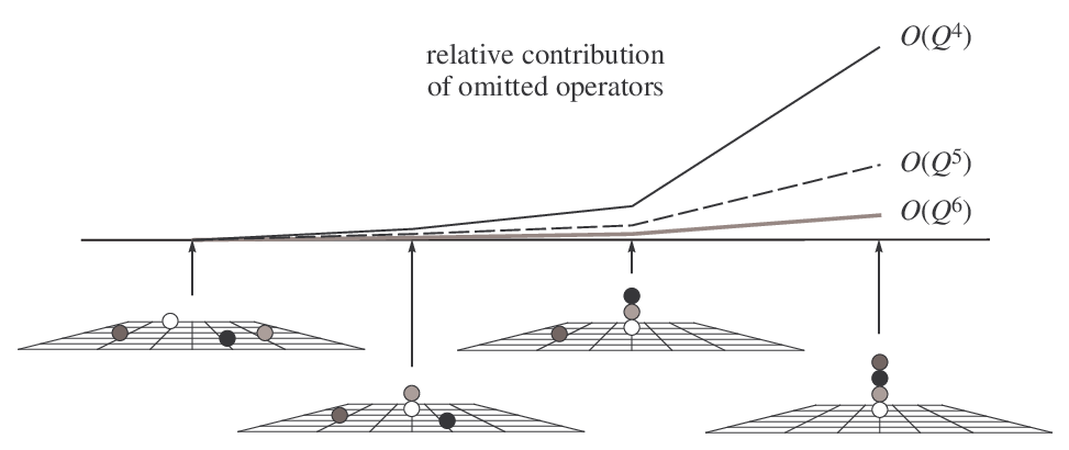
As the sketch suggests, the relative contribution is likely dominated by the last case where four nucleons are close together. If this hypothesis is correct then the contribution of higher-order operators to low-energy phenomena should be approximately universal. Different higher-order operators produce roughly the same effect on low-energy data. This situation is analogous to the difficulty one finds in resolving the value of $c_{D}$ from low-energy three-nucleon data. One useful consequence of this universality is that most of the residual error can be cancelled by adjusting the coefficient of an effective four-nucleon contact term,

V_{\text{effective}}^{(4N)}=\frac{1}{24}D_{\text{effective}}^{(4N)}:\sum_{\vec{n}}\left[\rho^{a^{\dagger},a}(\vec{n})\right]^{4}:\text{.}

(74)

This effective four-nucleon contact interaction should not be confused with the four-nucleon contact interaction that appears at $O(Q^{6})$ . We are not suggesting a rearrangement of power counting in chiral effective field theory. We are simply taking advantage of the expected universality of missing higher-order interactions. Later in our discussion we present results which test and appear to confirm this universality hypothesis.

The inclusion of $V_{\text{effective}}^{(4N)}$ provides an opportunity to resolve another related issue that was noted in earlier lattice calculations. Let $\left|4N_{\text{one-site}}\right\rangle$ be a configuration of four nucleons on a single lattice site,

\left|4N_{\text{one-site}}\right\rangle=a_{0,0}^{\dagger}(\vec{n})a_{1,0}^{\dagger}(\vec{n})a_{0,1}^{\dagger}(\vec{n})a_{1,1}^{\dagger}(\vec{n})\left|0\right\rangle.

(75)

The potential energy of this configuration is dependent upon the three-nucleon contact operator and the local part of the three-nucleon one-pion-exchange interaction,

\left\langle 4N_{\text{one-site}}\right|V_{\text{contact}}^{(3N)}\left|4N_{\text{one-site}}\right\rangle=4D_{\text{contact}}^{(3N)},

(76)

\left\langle 4N_{\text{one-site}}\right|V_{\text{OPE}}^{(3N)}\left|4N_{\text{one-site}}\right\rangle=12\frac{g_{A}\alpha_{t}}{f_{\pi}q_{\pi}}D_{\text{OPE}}^{(3N)}\sum\limits_{S}G_{SS}(\vec{0}).

(77)

If $D_{\text{contact}}^{(3N)}$ or $D_{\text{OPE}}^{(3N)}$ is sufficiently large and negative, a clustering instability can be produced in systems with four or more nucleons. This is a lattice artifact that appears on coarse lattices [49], and is similar to the clustering instability found with point-like two-nucleon contact interactions [9]. That problem was solved by using improved lattice actions with operator smearing. An analogous technique could be adopted for the three-nucleon interactions. In Ref. [10], however, a different approach was used. In that analysis the temporal lattice spacing was adjusted to ensure that the size of the cutoff-dependent three-nucleon operator coefficients were small.

In this study we use a simpler and more direct technique. Let us define

	$\displaystyle D_{\text{effective}}^{\prime(4N)}$	$\displaystyle=\left\langle 4N_{\text{one-site}}\right\|V_{\text{contact}}^{(3N)}+V_{\text{OPE}}^{(3N)}+V_{\text{effective}}^{(4N)}\left\|4N_{\text{one-site}}\right\rangle$
		$\displaystyle=4D_{\text{contact}}^{(3N)}+12D_{\text{OPE}}^{(3N)}\frac{g_{A}\alpha_{t}}{f_{\pi}q_{\pi}}\sum\limits_{S}G_{SS}(\vec{0})+D_{\text{effective}}^{(4N)}.$		(78)

The problem is that the local three-nucleon terms induce an effect much the same as a four-nucleon contact interaction, and quite possibly a strong four-nucleon interaction. To remedy this we treat $D_{\text{effective}}^{(4N)}$ as a bare counterterm that removes the dependence on $D_{\text{contact}}^{(3N)}$ and $D_{\text{OPE}}^{(3N)}$ . In the following we express all lattice results in terms of the renormalized coupling $D_{\text{effective}}^{\prime(4N)}.$

X Auxiliary fields and projection Monte Carlo

For systems with more than three nucleons, sparse-matrix calculations using the lattice transfer matrix are not practical at large volumes. Instead we use projection Monte Carlo with auxiliary fields. The auxiliary-field transfer matrix for the LO₃ action requires sixteen auxiliary fields. One auxiliary field is associated with the total nucleon density $N^{\dagger}N$ , three fields for the spin density $N^{\dagger}\vec{\sigma}N$ , three fields for the isospin density $N^{\dagger}\boldsymbol{\tau}N$ , and nine fields for the spin-isospin density $N^{\dagger}\vec{\sigma}\boldsymbol{\tau}N$ . Let us define $M^{(n_{t})}(\pi_{I}^{\prime},s,s_{S},s_{I},s_{S,I})$ as the leading-order auxiliary-field transfer matrix at time step $n_{t}$ ,

$\displaystyle M^{(n_{t})}(\pi_{I}^{\prime},s,s_{S},s_{I},s_{S,I})$	$\displaystyle=\colon\exp\left\{-H_{\text{free}}\alpha_{t}-\frac{g_{A}\alpha_{t}}{2f_{\pi}\sqrt{q_{\pi}}}{\displaystyle\sum_{\vec{n},S,I}}\Delta_{S}\pi_{I}^{\prime}(\vec{n},n_{t})\rho_{S,I}^{a^{{\dagger}},a}(\vec{n})\right.$
	$\displaystyle+\frac{1}{4}\sqrt{\left(-3C_{S=0,I=1}-3C_{S=1,I=0}\right)\alpha_{t}}\sum_{\vec{n}}s(\vec{n},n_{t})\rho^{a^{{\dagger}},a}(\vec{n})$
	$\displaystyle+\frac{i}{4}\sqrt{\left(-3C_{S=0,I=1}+C_{S=1,I=0}\right)\alpha_{t}}\sum_{\vec{n},S}s_{S}(\vec{n},n_{t})\rho_{S}^{a^{{\dagger}},a}(\vec{n})$
	$\displaystyle+\frac{i}{4}\sqrt{\left(C_{S=0,I=1}-3C_{S=1,I=0}\right)\alpha_{t}}\sum_{\vec{n},I}s_{I}(\vec{n},n_{t})\rho_{I}^{a^{{\dagger}},a}(\vec{n})$
	$\displaystyle\left.+\frac{i}{4}\sqrt{\left(-C_{S=0,I=1}-C_{S=1,I=0}\right)\alpha_{t}}\sum_{\vec{n},S,I}s_{S,I}(\vec{n},n_{t})\rho_{S,I}^{a^{{\dagger}},a}(\vec{n})\right\}\colon.$	(79)

We can write $M_{\text{LO}}$ as the normalized integral

M_{\text{LO}}=\frac{{\displaystyle\int}D\pi_{I}^{\prime}DsDs_{S}Ds_{I}Ds_{S,I}\;e^{-S_{\pi\pi}^{(n_{t})}-S_{ss}^{(n_{t})}}M^{(n_{t})}(\pi_{I}^{\prime},s,s_{S},s_{I},s_{S,I})}{{\displaystyle\int}D\pi_{I}^{\prime}DsDs_{S}Ds_{I}Ds_{S,I}\;e^{-S_{\pi\pi}^{(n_{t})}-S_{ss}^{(n_{t})}}},

(80)

where $S_{\pi\pi}^{(n_{t})}$ is the piece of the instantaneous pion action at time step $n_{t}$ ,

S_{\pi\pi}^{(n_{t})}(\pi_{I}^{\prime})=\frac{1}{2}\sum_{\vec{n},I}\pi_{I}^{\prime}(\vec{n},n_{t})\pi_{I}^{\prime}(\vec{n},n_{t})-\frac{\alpha_{t}}{q_{\pi}}\sum_{\vec{n},I,l}\pi_{I}^{\prime}(\vec{n},n_{t})\pi_{I}^{\prime}(\vec{n}+\hat{l},n_{t}),

(81)

and $S_{ss}^{(n_{t})}$ is the auxiliary-field action at time step $n_{t}$ ,

	$\displaystyle S_{ss}^{(n_{t})}$	$\displaystyle=\frac{1}{2}\sum_{\vec{n},\vec{n}^{\prime}}s(\vec{n},n_{t})f^{-1}(\vec{n}-\vec{n}^{\prime})s(\vec{n}^{\prime},n_{t})+\frac{1}{2}\sum_{\vec{n},\vec{n}^{\prime},S}s_{S}(\vec{n},n_{t})f^{-1}(\vec{n}-\vec{n}^{\prime})s_{S}(\vec{n}^{\prime},n_{t})$
		$\displaystyle+\frac{1}{2}\sum_{\vec{n},\vec{n}^{\prime},I}s_{I}(\vec{n},n_{t})f^{-1}(\vec{n}-\vec{n}^{\prime})s_{I}(\vec{n}^{\prime},n_{t})+\frac{1}{2}\sum_{\vec{n},\vec{n}^{\prime},S,I}s_{S,I}(\vec{n},n_{t})f^{-1}(\vec{n}-\vec{n}^{\prime})s_{S,I}(\vec{n}^{\prime},n_{t}),$		(82)

with

f^{-1}(\vec{n}-\vec{n}^{\prime})=\frac{1}{L^{3}}\sum_{\vec{q}}\frac{1}{f(\vec{q})}e^{-i\vec{q}\cdot(\vec{n}-\vec{n}^{\prime})}\text{.}

(83)

The contributions from NLO, NNLO, isospin-breaking, and Coulomb interactions are treated using perturbation theory. This is done by including external sources coupled to densities and current densities. Let us define

M_{\text{LO}}(\varepsilon)=\frac{{\displaystyle\int}D\pi_{I}^{\prime}DsDs_{S}Ds_{I}Ds_{S,I}\;e^{-S_{\pi\pi}^{(n_{t})}-S_{ss}^{(n_{t})}}M^{(n_{t})}(\pi_{I}^{\prime},s,s_{S},s_{I},s_{S,I},\varepsilon)}{{\displaystyle\int}D\pi_{I}^{\prime}DsDs_{S}Ds_{I}Ds_{S,I}\;e^{-S_{\pi\pi}^{(n_{t})}-S_{ss}^{(n_{t})}}},

(84)

where

		$\displaystyle M^{(n_{t})}(\pi_{I}^{\prime},s,s_{S},s_{I},s_{S,I},\varepsilon)$
		$\displaystyle=:M^{(n_{t})}(\pi_{I}^{\prime},s,s_{S},s_{I},s_{S,I})\exp\left[U^{(n_{t})}(\varepsilon)+U_{I^{2}}^{(n_{t})}(\varepsilon)\right]:.$		(85)

The isospin-independent couplings are

$\displaystyle U^{(n_{t})}(\varepsilon)$	$\displaystyle=\sum_{\vec{n}}\varepsilon_{\rho}(\vec{n},n_{t})\rho^{a^{\dagger},a}(\vec{n})+\sum_{\vec{n},S}\varepsilon_{\rho_{S}}(\vec{n},n_{t})\rho_{S}^{a^{\dagger},a}(\vec{n})+\sum_{\vec{n},S}\varepsilon_{\Delta_{S}\rho}(\vec{n},n_{t})\Delta_{S}\rho^{a^{\dagger},a}(\vec{n})$
	$\displaystyle+\sum_{\vec{n},S,S^{\prime}}\varepsilon_{\Delta_{S}\rho_{S^{\prime}}}(\vec{n},n_{t})\Delta_{S}\rho_{S^{\prime}}^{a^{\dagger},a}(\vec{n})+\sum_{\vec{n},l}\varepsilon_{\triangledown_{l}^{2}\rho}(\vec{n},n_{t})\triangledown_{l}^{2}\rho^{a^{\dagger},a}(\vec{n})$
	$\displaystyle+\sum_{\vec{n},l,S}\varepsilon_{\triangledown_{l}^{2}\rho_{S}}(\vec{n},n_{t})\triangledown_{l}^{2}\rho_{S}^{a^{\dagger},a}(\vec{n})+\sum_{\vec{n},l}\varepsilon_{\Pi_{l}}(\vec{n},n_{t})\Pi_{l}^{a^{\dagger},a}(\vec{n})+\sum_{\vec{n},l,S}\varepsilon_{\Pi_{l,S}}(\vec{n},n_{t})\Pi_{l,S}^{a^{\dagger},a}(\vec{n}),$	(86)

the isospin-dependent couplings are

$\displaystyle U_{I^{2}}^{(n_{t})}(\varepsilon)$	$\displaystyle=\sum_{\vec{n},I}\varepsilon_{\rho_{I}}(\vec{n},n_{t})\rho_{I}^{a^{\dagger},a}(\vec{n})+\sum_{\vec{n},S,I}\varepsilon_{\rho_{S,I}}(\vec{n},n_{t})\rho_{S,I}^{a^{\dagger},a}(\vec{n})+\sum_{\vec{n},S,I}\varepsilon_{\Delta_{S}\rho_{I}}(\vec{n},n_{t})\Delta_{S}\rho_{I}^{a^{\dagger},a}(\vec{n})$
	$\displaystyle+\sum_{\vec{n},S,S^{\prime},I}\varepsilon_{\Delta_{S}\rho_{S^{\prime},I}}(\vec{n},n_{t})\Delta_{S}\rho_{S^{\prime},I}^{a^{\dagger},a}(\vec{n})+\sum_{\vec{n},l,I}\varepsilon_{\triangledown_{l}^{2}\rho_{I}}(\vec{n},n_{t})\triangledown_{l}^{2}\rho_{I}^{a^{\dagger},a}(\vec{n})$
	$\displaystyle+\sum_{\vec{n},l,S,I}\varepsilon_{\triangledown_{l}^{2}\rho_{S,I}}(\vec{n},n_{t})\triangledown_{l}^{2}\rho_{S,I}^{a^{\dagger},a}(\vec{n})+\sum_{\vec{n},l,I}\varepsilon_{\Pi_{l,I}}(\vec{n},n_{t})\Pi_{l,I}^{a^{\dagger},a}(\vec{n})+\sum_{\vec{n},l,S,I}\varepsilon_{\Pi_{l,S,I}}(\vec{n},n_{t})\Pi_{l,S,I}^{a^{\dagger},a}(\vec{n}).$	(87)

All of the NLO, NNLO, isospin-breaking, and Coulomb interactions are generated by functional derivatives with respect to the external source fields.

We extract the properties of the ground state using Euclidean-time projection. Let $\left|\Psi^{\text{free}}\right\rangle$ be a Slater determinant of free-particle standing waves in a periodic cube for some chosen number of nucleons and quantum numbers. Let $M_{\text{SU(4)}\not\pi}^{(n_{t})}$ be an auxiliary-field transfer matrix at time step $n_{t}$ ,

M_{\text{SU(4)}\not\pi}^{(n_{t})}(s)=\colon\exp\left[-H_{\text{free}}\alpha_{t}+\sqrt{-C_{\text{SU(4)}\not\pi}\alpha_{t}}\sum_{\vec{n}}s(\vec{n},n_{t})\rho^{a^{{\dagger}},a}(\vec{n})\right]:.

(88)

We use the operator $M_{\text{SU(4)}\not\pi}^{(n_{t})}(s)$ to set up the initial state for the lattice calculation,

\left|\Psi(t^{\prime})\right\rangle=\left(M_{\text{SU(4)}\not\pi}\right)^{L_{t_{o}}}\left|\Psi^{\text{free}}\right\rangle,

(89)

where $t^{\prime}=L_{t_{o}}\alpha_{t}$ and $L_{t_{o}}$ is the number of “outer” time steps. As the notation suggests, the operator $M_{\text{SU(4)}\not\pi}^{(n_{t})}(s)$ is invariant under Wigner’s SU(4) symmetry [50]. The repeated multiplication by $M_{\text{SU(4)}\not\pi}^{(n_{t})}(s)$ acts as an approximate low-energy filter. This part of the Euclidean-time propagation is positive definite for any even number of nucleons invariant under the SU(4) symmetry [51, 52, 53].

The Euclidean-time amplitude $Z(t)$ is defined as

Z(t)=\left\langle\Psi(t^{\prime})\right|\left(M_{\text{LO}}\right)^{L_{t_{i}}}\left|\Psi(t^{\prime})\right\rangle,

(90)

where $t=L_{t_{i}}\alpha_{t}$ and $L_{t_{i}}$ is the number of “inner” time steps. The transient energy at time $t+\alpha_{t}/2$ is calculated by taking a numerical derivative of the logarithm of $Z(t)$ ,

e^{-E_{\text{LO}}(t+\alpha_{t}/2)\cdot\alpha_{t}}=\frac{Z(t+\alpha_{t})}{Z(t)}.

(91)

The ground state energy $E_{0,\text{LO}}$ equals the asymptotic limit of the transient energy,

E_{0,\text{LO}}=\lim_{t\rightarrow\infty}E_{\text{LO}}(t+\alpha_{t}/2).

(92)

We calculate Euclidean-time projection amplitudes using the auxiliary-field formalism. For a given configuration of auxiliary and pion fields, the contribution to the amplitude $Z(t)$ is proportional to the determinant of an $A\times A$ matrix of one-body amplitudes, where $A$ is the number of nucleons. Integrations over auxiliary and pion field configurations are computed using hybrid Monte Carlo. Details of the method can be found in Ref. [54, 55, 9, 11].

The perturbative contributions from NLO, NNLO, isospin-breaking, and Coulomb interactions are computed order-by-order in perturbation theory. For the first-order perturbative correction to the energy, it suffices to compute operator expectation values. For general operator $O$ we define the Euclidean-time amplitude,

Z_{O}(t)=\left\langle\Psi(t^{\prime})\right|\left(M_{\text{LO}}\right)^{L_{t_{i}}/2}O\,\left(M_{\text{LO}}\right)^{L_{t_{i}}/2}\left|\Psi(t^{\prime})\right\rangle.

(93)

The expectation value of $O$ for $\left|\Psi_{0}\right\rangle$ is extracted by taking the large $t$ limit of the ratio of $Z_{O}(t)$ and $Z(t)$ ,

\lim_{t\rightarrow\infty}\frac{Z_{O}(t)}{Z(t)}=\left\langle\Psi_{0}\right|O\left|\Psi_{0}\right\rangle.

(94)

In the appendix we show precise numerical tests of the equivalence of the auxiliary-field Monte Carlo formalism and the original transfer matrix formalism.

XI Results for helium-4

We compute the ground state energy for helium-4 in a periodic box of length $9.9$ fm. For $\left|\Psi^{\text{free}}\right\rangle$ we take the Slater determinant formed by standing waves,

\left\langle 0\right|a_{i,j}(\vec{n})\left|\psi_{1}\right\rangle\propto\delta_{i,0}\delta_{j,1},\qquad\left\langle 0\right|a_{i,j}(\vec{n})\left|\psi_{2}\right\rangle\propto\delta_{i,0}\delta_{j,0},

(95)

\left\langle 0\right|a_{i,j}(\vec{n})\left|\psi_{3}\right\rangle\propto\delta_{i,1}\delta_{j,1},\qquad\left\langle 0\right|a_{i,j}(\vec{n})\left|\psi_{4}\right\rangle\propto\delta_{i,1}\delta_{j,0}\text{.}

(96)

This produces a state with zero total momentum and the quantum numbers of the helium-4 ground state. For each value of the Euclidean time, $t$ , we use $2048$ processors to generate about $5\times 10^{6}$ hybrid Monte Carlo trajectories. Each processor runs independent trajectories, and averages and stochastic errors are calculated from the distribution of results from all processors.

For the numerical extrapolation in $t$ , we use a decaying exponential for the leading-order energy,

E_{\text{LO}}(t)\approx E_{0,\text{LO}}+A_{\text{LO}}e^{-\delta E\cdot t}.

(97)

For each of the perturbative energy corrections from NLO, isospin-breaking (IB), electromagnetic (EM), and NNLO interactions we use

\Delta E(t)\approx\Delta E_{0}+\Delta Ae^{-\delta E\cdot t/2}.

(98)

The unknown parameters $E_{0,\text{LO}}$ , $A_{\text{LO}}$ , $\Delta A$ , and $\delta E$ , are determined by least squares fitting. The $e^{-\delta E\cdot t}$ dependence in Eq. (97) gives the contribution of low-energy excitations with energy gap $\delta E$ above the ground state. The $e^{-\delta E\cdot t/2}$ dependence in Eq. (98) gives the contribution of matrix elements between the ground state and excitations at energy gap $\delta E$ .

Given the finite interval over which we measure the Euclidean-time dependence, we expect some exponential dependence from other energy excitations not at energy $\delta E$ above the ground state. In order to estimate the size of the induced systematic errors, we generate an ensemble of different exponential fits which include dropping the two first two data points and then dropping the last two data points. This gives some estimate of the spread in energies of contributing higher energy states. In the following we quote total extrapolation errors which include the uncertainty due to the stochastic errors and the effect of the distribution in $\delta E$ . In future studies we hope to improve this process further by considering different initial states in order to triangulate a common extrapolated value at infinite $t$ .

In Fig. 9 we show the energy versus Euclidean time projection for the helium-4 ground state with LO, NLO, IB, EM, and NNLO interactions. The plot on the left shows the leading-order results and the extrapolated $t\rightarrow\infty$ values for the higher-order contributions added cumulatively. These cumulative results are shown with error bars on the right edge of the plot. The plot on the right shows the higher-order corrections separately. For each case we show the best fit as well as the one standard-deviation bound. We estimate this bound by generating an ensemble of fits determined with added random Gaussian noise proportional to the error bars of each data point and also varying the number of fitted data points. These results are similar to those found in Ref. [10] using the LO₂ action. For $c_{D}=1$ we get $-30.5(4)$ MeV at LO, $-30.6(4)$ MeV at NLO, $-29.2(4)$ MeV at NLO with IB and EM corrections, and $-30.1(5)$ MeV at NNLO. When the bare interaction $D_{\text{effective}}^{(4N)}$ is held fixed, the helium-4 energy decreases $0.4(1)$ MeV for each unit increase in $c_{D}$ .

Apart from direct comparisons with experimental data, an independent estimate of systematic errors due to truncation of higher-order terms can be made by comparing the differences among the lattice results at each order, LO, NLO, and NNLO. One caveat here is that sometimes the differences can be unusually small, either by chance or due to underlying physics. For example there is only a very small difference between the LO and NLO energies for helium-4. This can be explained by the fact that the interactions for helium-4 are predominantly in the $S$ -channels, and the improved LO₃ action is already quite accurate for $S$ -wave scattering. For helium-4 we estimate a residual error of size about $1$ MeV for the omitted interactions. This appears consistent with the $1.8$ MeV deviation between the NNLO result and the physical binding energy for helium-4.

For nuclei beyond $A=4$ , we will test the universality hypothesis for higher-order interactions by tuning the effective four-nucleon contact interaction $D_{\text{effective}}^{\prime(4N)}$ to give the physical helium-4 energy of $-28.3$ MeV. The contribution of the effective four-nucleon contact interaction to the helium-4 energy is shown in Fig. 9.

XII Results for lithium-6

We compute the ground state energy for lithium-6 in a periodic box of length $9.9$ fm. For $\left|\Psi^{\text{free}}\right\rangle$ we choose standing waves,

\left\langle 0\right|a_{i,j}(\vec{n})\left|\psi_{1}\right\rangle\propto\delta_{i,1}\delta_{j,1},\qquad\left\langle 0\right|a_{i,j}(\vec{n})\left|\psi_{2}\right\rangle\propto\delta_{i,1}\delta_{j,0}\text{.}

(99)

\left\langle 0\right|a_{i,j}(\vec{n})\left|\psi_{3}\right\rangle\propto\delta_{i,0}\delta_{j,1}\cos\tfrac{2\pi n_{3}}{L},\qquad\left\langle 0\right|a_{i,j}(\vec{n})\left|\psi_{4}\right\rangle\propto\delta_{i,0}\delta_{j,0}\cos\tfrac{2\pi n_{3}}{L},

(100)

\left\langle 0\right|a_{i,j}(\vec{n})\left|\psi_{5}\right\rangle\propto\delta_{i,0}\delta_{j,1}\sin\tfrac{2\pi n_{3}}{L},\qquad\left\langle 0\right|a_{i,j}(\vec{n})\left|\psi_{6}\right\rangle\propto\delta_{i,0}\delta_{j,0}\sin\tfrac{2\pi n_{3}}{L}.

(101)

This combination produces a state with zero total momentum and the quantum numbers of the lithium-6 ground state. For each value of $t$ a total of about $5\times 10^{6}$ hybrid Monte Carlo trajectories are generated by $2048$ processors.

In Fig. 10 we show the energy versus Euclidean time projection for lithium-6. For the numerical extrapolation in $t$ we use the same decaying exponential functions in Eq. (97-98). We show the best fit as well as the one standard-deviation bound. For $c_{D}=1$ we get $-32.6(9)$ MeV at LO, $-34.6(9)$ MeV at NLO, $-32.4(9)$ MeV at NLO with IB and EM corrections, and $-34.5(9)$ MeV at NNLO. Our error estimate due to truncation at NNLO is about $2$ MeV. Adding the contribution of the effective four-nucleon interaction $D_{\text{effective}}^{\prime(4N)}$ to the NNLO result gives $-32.9(9)$ MeV. This lies within error bars of the physical value $-32.0$ MeV. However we expect some overbinding due to the finite periodic volume. The finite volume analysis in Ref. [10] found a finite volume dependence of less than $1$ MeV for the helium-4 ground state in a periodic box of length $9.9$ fm. However a larger effect is expected for lithium-6 due to the larger spatial distribution of the two $P$ -shell nucleons. Further calculations at varying volumes will be needed to determine this volume dependence.

Compared with helium-4, there is a much larger difference between the LO and NLO energies for lithium-6. This may indicate additional binding coming from the NLO corrections in $P$ -wave channels. The dependence of the energy on $c_{D}$ can be analyzed in several different ways. When the bare interaction $D_{\text{effective}}^{(4N)}$ is held fixed, the lithium-6 energy decreases $0.7(1)$ MeV for each unit increase in $c_{D}$ . When the effective four-nucleon interaction is adjusted according to the physical helium-4 energy, the lithium-6 energy decreases $0.35(5)$ MeV per unit increase in $c_{D}$ .

XIII Results for carbon-12

We compute the ground state energy of carbon-12 in a periodic box of length $13.8$ fm. For $\left|\Psi^{\text{free}}\right\rangle$ we take the Slater determinant formed by standing waves,

\left\langle 0\right|a_{i,j}(\vec{n})\left|\psi_{4k+1}\right\rangle\propto\delta_{i,0}\delta_{j,1}f_{k}(\vec{n}),\qquad\left\langle 0\right|a_{i,j}(\vec{n})\left|\psi_{4k+2}\right\rangle\propto\delta_{i,0}\delta_{j,0}f_{k}(\vec{n}),

(102)

\left\langle 0\right|a_{i,j}(\vec{n})\left|\psi_{4k+3}\right\rangle\propto\delta_{i,1}\delta_{j,1}f_{k}(\vec{n}),\qquad\left\langle 0\right|a_{i,j}(\vec{n})\left|\psi_{4k+4}\right\rangle\propto\delta_{i,1}\delta_{j,0}f_{k}(\vec{n})\text{,}

(103)

where

f_{0}(\vec{n})=1,\quad f_{1}(\vec{n})=\cos\tfrac{2\pi n_{3}}{L},\quad f_{2}(\vec{n})=\sin\tfrac{2\pi n_{3}}{L}.

(104)

This combination produces a state with zero total momentum and the quantum numbers of the carbon-12 ground state. For each value of $t$ a total of $2\times 10^{6}$ hybrid Monte Carlo trajectories are generated by $2048$ processors.

Fig. 11 shows the energy versus Euclidean time projection for carbon-12. For $c_{D}=1$ we get $-109(2)$ MeV at LO, $-115(2)$ MeV at NLO, $-108(2)$ MeV at NLO with IB and EM corrections, and $-106(2)$ MeV at NNLO. Our error estimate due to truncation at NNLO is about $5$ MeV. The small $2$ MeV difference between NLO and NNLO results is due to a cancellation of several larger contributions. Adding the contribution of the effective four-nucleon interaction $D_{\text{effective}}^{\prime(4N)}$ to the NNLO result gives $-99(2)$ MeV. This is an overbinding of $7\%$ compared to the physical value, $-92.2$ MeV. While this agreement as a final result would not be bad, an overbinding of $7\%$ is actually a reasonable estimate of the finite volume correction for carbon-12 in a periodic box of length $13.8$ fm. If so the error at infinite volume would in fact be much smaller than $7\%$ . Further calculations at varying volumes will be needed to measure the volume dependence.

When the bare interaction $D_{\text{effective}}^{(4N)}$ is held fixed, the carbon-12 energy decreases $1.7(3)$ MeV per unit increase in $c_{D}$ . When the effective four-nucleon interaction is adjusted according to the physical helium-4 energy, the carbon-12 energy decreases only $0.3(1)$ MeV per unit increase in $c_{D}$ . The much reduced dependence upon on $c_{D}$ is consistent with our universality hypothesis regarding systematic errors. In three-nucleon systems the value of $c_{D}$ is difficult to resolve due to similarities of the one-pion exchange three-nucleon interaction and the three-nucleon contact interaction at low energies. For systems with four or more nucleons, the difference between these three-nucleon interactions becomes significant. However our universality hypothesis suggests that this difference behaves like an effective four-nucleon contact interaction. This explains why the dependence on $c_{D}$ goes away when we include an effective four-nucleon contact interaction tuned to the physical helium-4 energy.

XIV Summary and comments

In this paper we have presented several new methods and results in lattice effective field theory. We described the first lattice results for lithium-6 and carbon-12 using chiral effective field theory. This represents a significant advance in the range of problems accessible using lattice effective field theory. We also detailed the first lattice calculations to include isospin-breaking and Coulomb interactions, and computed the energy splitting between helium-3 and the triton. The accuracy of the lattice calculations presented here are competitive with recent calculations obtained using other ab initio methods. Coupled cluster calculations without three-nucleon interactions are accurate to within $1$ MeV per nucleon for medium mass nuclei [56]. Constrained-path Green’s function Monte Carlo calculations generally have an accuracy of $1\%-2\%$ in energy for nuclei $A\leq 12$ . The most recent result for carbon-12 is $-93.2(6)$ MeV using AV18 and the IL7 three-nucleon force [57]. The most recent no-core shell model calculation for carbon-12 with the JISP16 $NN$ interaction considers two different extrapolation methods to obtain values $-93.9(1.1)$ MeV and $-95.1(2.7)$ MeV [58]. We also mention some recent lattice QCD simulations in the strong coupling limit. While quite different from physical nuclei, the strong coupling analog of nuclei have been simulated for up to twelve nucleons [59].

Future lattice studies should look at probing large volumes, decreasing the lattice spacing, and including higher-order interactions. The computational scaling with the number of nucleons suggests that larger nuclei are also possible. At fixed volume we find that the time required by one processor to generate one HMC trajectory scales with the number of nucleons as $A^{1.7}$ for $A\leq 16$ . For carbon-12 calculations the time required by one processor to generate one HMC trajectory scales with volume as $V^{1.5}$ . For nuclei with $S=0$ and $I=0$ the average sign $\left\langle e^{i\theta}\right\rangle$ scales as $e^{-0.11A}$ . From this scaling data we estimate that a simulation of oxygen-16 would require about $1.8$ TFlop-yr.

Lattice effective field theory should prove a useful tool for few-body calculations of nuclei as well as many-body calculations of neutron and nuclear matter. The method is also quite attractive theoretically as it uses only the general principles of effective field theory. All systematic errors are introduced up front when defining the truncated low-energy effective theory. This eliminates approximation errors tied with a specific calculational tool, physical system, or observable. The reduction of these errors is not necessarily easy. However they can be clearly identified as either missing operators in the lattice action, finite volume effects, or errors from finite Euclidean-time extrapolation. Future studies can then improve upon existing calculations in a straightforward manner.

Acknowledgements

Partial financial support from the Deutsche Forschungsgemeinschaft (SFB/TR 16), Helmholtz Association (contract number VH-NG-222 and VH-VI-231), BMBF (grant 06BN9006), and U.S. Department of Energy (DE-FG02-03ER41260) are acknowledged. This work was further supported by the EU HadronPhysics2 project “Study of strongly interacting matter”. The computational resources for this project were provided by the Jülich Supercomputing Centre at the Forschungszentrum Jülich.

Appendix A Lattice notation

The vector $\vec{n}$ represents integer-valued lattice vectors on a three-dimensional spatial lattice, and $\vec{p},$ $\vec{q},$ $\vec{k}$ represent integer-valued momentum lattice vectors. $\ \ \hat{l}=\hat{1}$ , $\hat{2}$ , $\hat{3}$ are unit lattice vectors in the spatial directions, $a$ is the spatial lattice spacing, and $L$ is the length of the cubic spatial lattice in each direction. The lattice time step is $a_{t}$ , and $n_{t}$ labels the number of time steps. We define $\alpha_{t}$ as the ratio between lattice spacings, $\alpha_{t}=a_{t}/a$ . Throughout our lattice discussion we use dimensionless parameters and operators, which correspond with physical values multiplied by the appropriate power of $a$ . Final results are presented in physical units with the corresponding unit stated explicitly.

We use $a$ and $a^{\dagger}$ to denote annihilation and creation operators. We make explicit all spin and isospin indices,

	$\displaystyle a_{0,0}$	$\displaystyle=a_{\uparrow,p},\text{ \ }a_{0,1}=a_{\uparrow,n},$		(105)
	$\displaystyle a_{1,0}$	$\displaystyle=a_{\downarrow,p},\text{ \ }a_{1,1}=a_{\downarrow,n}.$		(106)

The first subscript is for spin and the second subscript is for isospin. We use $\tau_{I}$ with $I=1,2,3$ to represent Pauli matrices acting in isospin space and $\sigma_{S}$ with $S=1,2,3$ to represent Pauli matrices acting in spin space. For the free nucleon we use the $O(a^{4})$ -improved lattice Hamiltonian,

$\displaystyle H_{\text{free}}$	$\displaystyle=\frac{49}{12m}\sum_{\vec{n}}\sum_{i,j=0,1}a_{i,j}^{\dagger}(\vec{n})a_{i,j}(\vec{n})$
	$\displaystyle-\frac{3}{4m}\sum_{\vec{n}}\sum_{i,j=0,1}\sum_{l=1,2,3}\left[a_{i,j}^{\dagger}(\vec{n})a_{i,j}(\vec{n}+\hat{l})+a_{i,j}^{\dagger}(\vec{n})a_{i,j}(\vec{n}-\hat{l})\right]$
	$\displaystyle+\frac{3}{40m}\sum_{\vec{n}}\sum_{i,j=0,1}\sum_{l=1,2,3}\left[a_{i,j}^{\dagger}(\vec{n})a_{i,j}(\vec{n}+2\hat{l})+a_{i,j}^{\dagger}(\vec{n})a_{i,j}(\vec{n}-2\hat{l})\right]$
	$\displaystyle-\frac{1}{180m}\sum_{\vec{n}}\sum_{i,j=0,1}\sum_{l=1,2,3}\left[a_{i,j}^{\dagger}(\vec{n})a_{i,j}(\vec{n}+3\hat{l})+a_{i,j}^{\dagger}(\vec{n})a_{i,j}(\vec{n}-3\hat{l})\right].$	(107)

The eight vertices of a unit cube on the lattice is used to define spatial derivatives. For each spatial direction $l=1,2,3$ and any lattice function $f(\vec{n})$ , let

\Delta_{l}f(\vec{n})=\frac{1}{4}\sum_{\begin{subarray}{c}\nu_{1},\nu_{2},\nu_{3}=0,1\end{subarray}}(-1)^{\nu_{l}+1}f(\vec{n}+\vec{\nu}),\qquad\vec{\nu}=\nu_{1}\hat{1}+\nu_{2}\hat{2}+\nu_{3}\hat{3}.

(108)

We also define the double spatial derivative along direction $l$ ,

\triangledown_{l}^{2}f(\vec{n})=f(\vec{n}+\hat{l})+f(\vec{n}-\hat{l})-2f(\vec{n}).

(109)

For the three-body NNLO interactions we also use the notation

\square f(\vec{n})=\frac{1}{8}\sum_{\begin{subarray}{c}\nu_{1},\nu_{2},\nu_{3}=0,1\end{subarray}}f(\vec{n}+\vec{\nu}),\qquad\vec{\nu}=\nu_{1}\hat{1}+\nu_{2}\hat{2}+\nu_{3}\hat{3}.

(110)

A.1 Local densities and currents

We define the local density,

\rho^{a^{\dagger},a}(\vec{n})=\sum_{i,j=0,1}a_{i,j}^{\dagger}(\vec{n})a_{i,j}(\vec{n}),

(111)

which is invariant under Wigner’s SU(4) symmetry [50]. Similarly we define the local spin density for $S=1,2,3,$

\rho_{S}^{a^{\dagger},a}(\vec{n})=\sum_{i,j,i^{\prime}=0,1}a_{i,j}^{\dagger}(\vec{n})\left[\sigma_{S}\right]_{ii^{\prime}}a_{i^{\prime},j}(\vec{n}),

(112)

isospin density for $I=1,2,3,$

\rho_{I}^{a^{\dagger},a}(\vec{n})=\sum_{i,j,j^{\prime}=0,1}a_{i,j}^{\dagger}(\vec{n})\left[\tau_{I}\right]_{jj^{\prime}}a_{i,j^{\prime}}(\vec{n}),

(113)

and spin-isospin density for $S,I=1,2,3,$

\rho_{S,I}^{a^{\dagger},a}(\vec{n})=\sum_{i,j,i^{\prime},j^{\prime}=0,1}a_{i,j}^{\dagger}(\vec{n})\left[\sigma_{S}\right]_{ii^{\prime}}\left[\tau_{I}\right]_{jj^{\prime}}a_{i^{\prime},j^{\prime}}(\vec{n}).

(114)

For each static density we also have an associated current density. Similar to the definition of the lattice derivative $\Delta_{l}$ in Eq. (108), we use the eight vertices of a unit cube,

\vec{\nu}=\nu_{1}\hat{1}+\nu_{2}\hat{2}+\nu_{3}\hat{3},

(115)

for $\nu_{1},\nu_{2},\nu_{3}=0,1$ . Let $\vec{\nu}(-l)$ for $l=1,2,3$ be the result of reflecting the $l^{\text{th}}$ -component of $\vec{\nu}$ about the center of the cube,

\vec{\nu}(-l)=\vec{\nu}+(1-2\nu_{l})\hat{l}.

(116)

Omitting factors of $i$ and $1/m$ , we can write the $l^{\text{th}}$ -component of the SU(4)-invariant current density as

\Pi_{l}^{a^{\dagger},a}(\vec{n})=\frac{1}{4}\sum_{\begin{subarray}{c}\nu_{1},\nu_{2},\nu_{3}=0,1\end{subarray}}\sum_{i,j=0,1}(-1)^{\nu_{l}+1}a_{i,j}^{\dagger}(\vec{n}+\vec{\nu}(-l))a_{i,j}(\vec{n}+\vec{\nu}).

(117)

Similarly the $l^{\text{th}}$ -component of spin current density is

\Pi_{l,S}^{a^{\dagger},a}(\vec{n})=\frac{1}{4}\sum_{\begin{subarray}{c}\nu_{1},\nu_{2},\nu_{3}=0,1\end{subarray}}\sum_{i,j,i^{\prime}=0,1}(-1)^{\nu_{l}+1}a_{i,j}^{\dagger}(\vec{n}+\vec{\nu}(-l))\left[\sigma_{S}\right]_{ii^{\prime}}a_{i^{\prime},j}(\vec{n}+\vec{\nu}),

(118)

$l^{\text{th}}$ -component of isospin current density is

\Pi_{l,I}^{a^{\dagger},a}(\vec{n})=\frac{1}{4}\sum_{\begin{subarray}{c}\nu_{1},\nu_{2},\nu_{3}=0,1\end{subarray}}\sum_{i,j,j^{\prime}=0,1}(-1)^{\nu_{l}+1}a_{i,j}^{\dagger}(\vec{n}+\vec{\nu}(-l))\left[\tau_{I}\right]_{jj^{\prime}}a_{i,j^{\prime}}(\vec{n}+\vec{\nu}),

(119)

and $l^{\text{th}}$ -component of spin-isospin current density is

\Pi_{l,S,I}^{a^{\dagger},a}(\vec{n})=\frac{1}{4}\sum_{\begin{subarray}{c}\nu_{1},\nu_{2},\nu_{3}=0,1\end{subarray}}\sum_{i,j,i^{\prime},j^{\prime}=0,1}(-1)^{\nu_{l}+1}a_{i,j}^{\dagger}(\vec{n}+\vec{\nu}(-l))\left[\sigma_{S}\right]_{ii^{\prime}}\left[\tau_{I}\right]_{jj^{\prime}}a_{i^{\prime},j^{\prime}}(\vec{n}+\vec{\nu}).

(120)

A.2 Instantaneous free pion action

The lattice action for free pions with purely instantaneous propagation is

S_{\pi\pi}(\pi_{I})=\alpha_{t}(\tfrac{m_{\pi}^{2}}{2}+3)\sum_{\vec{n},n_{t},I}\pi_{I}(\vec{n},n_{t})\pi_{I}(\vec{n},n_{t})-\alpha_{t}\sum_{\vec{n},n_{t},I,l}\pi_{I}(\vec{n},n_{t})\pi_{I}(\vec{n}+\hat{l},n_{t}),

(121)

where $\pi_{I}$ is the pion field labelled with isospin index $I$ , and $m_{\pi}=m_{\pi^{0}}$ . It is convenient to define a rescaled pion field, $\pi_{I}^{\prime}$ ,

\pi_{I}^{\prime}(\vec{n},n_{t})=\sqrt{q_{\pi}}\pi_{I}(\vec{n},n_{t}),

(122)

q_{\pi}=\alpha_{t}(m_{\pi}^{2}+6).

(123)

Then

S_{\pi\pi}(\pi_{I}^{\prime})=\frac{1}{2}\sum_{\vec{n},n_{t},I}\pi_{I}^{\prime}(\vec{n},n_{t})\pi_{I}^{\prime}(\vec{n},n_{t})-\frac{\alpha_{t}}{q_{\pi}}\sum_{\vec{n},n_{t},I,l}\pi_{I}^{\prime}(\vec{n},n_{t})\pi_{I}^{\prime}(\vec{n}+\hat{l},n_{t}).

(124)

In momentum space the action is

S_{\pi\pi}(\pi_{I}^{\prime})=\frac{1}{L^{3}}\sum_{I,\vec{k}}\pi_{I}^{\prime}(-\vec{k},n_{t})\pi_{I}^{\prime}(\vec{k},n_{t})\left[\frac{1}{2}-\frac{\alpha_{t}}{q_{\pi}}\sum_{l}\cos k_{l}\right].

(125)

The instantaneous pion correlation function at spatial separation $\vec{n}$ is

	$\displaystyle\left\langle\pi_{I}^{\prime}(\vec{n},n_{t})\pi_{I}^{\prime}(\vec{0},n_{t})\right\rangle$	$\displaystyle=\frac{\int D\pi_{I}^{\prime}\;\pi_{I}^{\prime}(\vec{n},n_{t})\pi_{I}^{\prime}(\vec{0},n_{t})\;\exp\left[-S_{\pi\pi}\right]}{\int D\pi_{I}^{\prime}\;\exp\left[-S_{\pi\pi}\right]}\text{ \ (no sum on }I\text{)}$
		$\displaystyle=\frac{1}{L^{3}}\sum_{\vec{k}}e^{-i\vec{k}\cdot\vec{n}}D_{\pi}(\vec{k}),$		(126)

where

D_{\pi}(\vec{k})=\frac{1}{1-\tfrac{2\alpha_{t}}{q_{\pi}}\sum_{l}\cos k_{l}}.

(127)

It is also useful to define the two-derivative pion correlator, $G_{S_{1}S_{2}}(\vec{n})$ ,

	$\displaystyle G_{S_{1}S_{2}}(\vec{n})$	$\displaystyle=\left\langle\Delta_{S_{1}}\pi_{I}^{\prime}(\vec{n},n_{t})\Delta_{S_{2}}\pi_{I}^{\prime}(\vec{0},n_{t})\right\rangle\text{ \ (no sum on }I\text{)}$
		$\displaystyle=\frac{1}{16}\sum_{\nu_{1},\nu_{2},\nu_{3}=0,1}\sum_{\nu_{1}^{\prime},\nu_{2}^{\prime},\nu_{3}^{\prime}=0,1}(-1)^{\nu_{S_{1}}}(-1)^{\nu_{S_{2}}^{\prime}}\left\langle\pi_{I}^{\prime}(\vec{n}+\vec{\nu}-\vec{\nu}^{\prime},n_{t})\pi_{I}^{\prime}(\vec{0},n_{t})\right\rangle.$		(128)

A.3 Pion mass differences

We outline the modifications that result from different masses for the charged pion and neutral pion. Let

q_{\pi}(m_{\pi^{\pm}})=\alpha_{t}(m_{\pi^{\pm}}^{2}+6),\qquad q_{\pi}(m_{\pi^{0}})=\alpha_{t}(m_{\pi^{0}}^{2}+6).

(129)

The rescaled pion fields are then

\pi_{1,2}^{\prime}(\vec{n},n_{t})=\sqrt{q_{\pi}(m_{\pi^{\pm}})}\pi_{1,2}(\vec{n},n_{t}),\qquad\pi_{3}^{\prime}(\vec{n},n_{t})=\sqrt{q_{\pi}(m_{\pi^{0}})}\pi_{3}(\vec{n},n_{t}).

(130)

The momentum-space correlators for the charged and neutral pions are

D_{\pi}(\vec{k},m_{\pi^{\pm}})=\frac{1}{1-\tfrac{2\alpha_{t}}{q_{\pi}(m_{\pi^{\pm}})}\sum_{l}\cos k_{l}},

(131)

D_{\pi}(\vec{k},m_{\pi^{0}})=\frac{1}{1-\tfrac{2\alpha_{t}}{q_{\pi}(m_{\pi^{0}})}\sum_{l}\cos k_{l}}.

(132)

We can now repeat the steps in Eq. (128) to define the two-derivative pion correlators $G_{S_{1}S_{2}}(\vec{n},m_{\pi^{\pm}})$ and $G_{S_{1}S_{2}}(\vec{n},m_{\pi^{0}})$ .

Appendix B Precision tests

We use the three-nucleon system as a precision test of the lattice formalism and computer codes. The same observables are calculated using both auxiliary-field Monte Carlo and the exact transfer matrix without auxiliary fields. We choose a small system so that stochastic errors are small enough to expose disagreement at the $0.1\%-1\%$ level. We choose the spatial length of the lattice to be $L=3$ lattice units and set the outer time steps $L_{t_{o}}=0$ and inner time steps $L_{t_{i}}=4$ . With $2048$ processors we generate a total of about $10^{7}$ hybrid Monte Carlo trajectories. Each processor runs completely independent trajectories, and we compute averages and stochastic errors by comparing the results of all processors.

We choose $\left|\Psi^{\text{free}}\right\rangle$ to be a Slater determinant of free-particle standing waves where

\left\langle 0\right|a_{i,j}(\vec{n})\left|\psi_{1}\right\rangle\propto\delta_{i,0}\delta_{j,0},\qquad\left\langle 0\right|a_{i,j}(\vec{n})\left|\psi_{2}\right\rangle\propto\delta_{i,1}\delta_{j,0},\qquad\left\langle 0\right|a_{i,j}(\vec{n})\left|\psi_{3}\right\rangle\propto\delta_{i,0}\delta_{j,1}\text{.}

(133)

The quantum numbers of this state correspond with helium-3 at zero momentum. At leading order we find an energy of $-49.72(6)$ MeV for the Monte Carlo calculation and $-49.7515$ MeV for the exact transfer matrix. In Table 1 we compare Monte Carlo results (MC) and exact transfer matrix calculations (Exact) for the derivative of the energy with respect to each NLO coefficient. Table 2 shows the energy shifts due to the proton-proton contact interaction and the Coulomb interaction, and Table 3 shows the derivative of the energy with respect to each NNLO coefficient. The numbers in parentheses are the estimated stochastic errors. In all cases the agreement between Monte Carlo results and exact transfer calculations is consistent with estimated stochastic errors.

Table 1: Monte Carlo results versus exact transfer matrix calculations for the derivative of the energy with respect to NLO coefficients.

NLO energy derivatives	MC	Exact
$\frac{\partial\left(\Delta E_{\text{NLO}}(t)\right)}{\partial\left(\Delta C\right)}$ [ $10^{4}$ MeV³]	$3.722(3)$	$3.72347$
$\frac{\partial\left(\Delta E_{\text{NLO}}(t)\right)}{\partial\left(\Delta C_{I^{2}}\right)}$ [ $10^{4}$ MeV³]	$-4.530(6)$	$-4.53590$
$\frac{\partial\left(\Delta E_{\text{NLO}}(t)\right)}{\partial\left(C_{q^{2}}\right)}$ [ $10^{9}$ MeV⁵]	$-2.055(2)$	$-2.05383$
$\frac{\partial\left(\Delta E_{\text{NLO}}(t)\right)}{\partial\left(C_{I^{2},q^{2}}\right)}$ [ $10^{9}$ MeV⁵]	$3.052(3)$	$3.05148$
$\frac{\partial\left(\Delta E_{\text{NLO}}(t)\right)}{\partial\left(C_{S^{2},q^{2}}\right)}$ [ $10^{9}$ MeV⁵]	$0.161(3)$	$0.16376$
$\frac{\partial\left(\Delta E_{\text{NLO}}(t)\right)}{\partial\left(C_{S^{2},I^{2},q^{2}}\right)}$ [ $10^{9}$ MeV⁵]	$5.240(5)$	$5.24260$
$\frac{\partial\left(\Delta E_{\text{NLO}_{3}}(t)\right)}{\partial\left(C_{(q\cdot S)^{2}}\right)}$ [ $10^{9}$ MeV⁵]	$-1.5873(9)$	$-1.58896$
$\frac{\partial\left(\Delta E_{\text{NLO}}(t)\right)}{\partial\left(C_{I^{2},(q\cdot S)^{2}}\right)}$ [ $10^{9}$ MeV⁵]	$6.833(3)$	$6.83234$
$\frac{\partial\left(\Delta E_{\text{NLO}}(t)\right)}{\partial\left(C_{(iq\times S)\cdot k}\right)}$ [ $10^{9}$ MeV⁵]	$0.3356(5)$	$0.33702$
$\frac{\partial\left(\Delta E_{\text{NLO}}(t)\right)}{\partial\left(C_{I^{2},(iq\times S)\cdot k}\right)}$ [ $10^{9}$ MeV⁵]	$-0.996(2)$	$-0.99656$

Table 2: Monte Carlo results versus exact transfer matrix calculations for the energy shifts due to the proton-proton contact interaction and the Coulomb interaction.

IB and EM energy shifts	MC	Exact
$\Delta E_{\text{pp}}(t)$ [ $10^{-2}$ MeV]	1.937(2)	1.94128
$\Delta E_{\text{EM}}(t)$ [ $10^{-1}$ MeV]	3.712(2)	3.71232

Table 3: Monte Carlo results versus exact transfer matrix calculations for the derivative of the energy with respect to NNLO coefficients.

NNLO energy derivatives	MC	Exact
$\frac{\partial\left(\Delta E_{\text{NNLO}}(t)\right)}{\partial\left(D_{\text{contact}}\right)}$ [ $10^{8}$ MeV⁶]	$0.999(7)$	$1.0029$
$\frac{\partial\left(\Delta E_{\text{NNLO}}(t)\right)}{\partial\left(D_{\text{OPE}}\right)}$ [ $10^{7}$ MeV⁵]	$-5.81(2)$	$-5.8070$
$\frac{\partial\left(\Delta E_{\text{NNLO}}(t)\right)}{\partial\left(D_{\text{TPE1}}\right)}$ [ $10^{5}$ MeV⁴]	$15.27(13)$	$15.319$
$\frac{\partial\left(\Delta E_{\text{NNLO}}(t)\right)}{\partial\left(D_{\text{TPE2}}\right)}$ [ $10^{5}$ MeV⁴]	$2.33(6)$	$2.2744$
$\frac{\partial\left(\Delta E_{\text{NNLO}}(t)\right)}{\partial\left(D_{\text{TPE3}}\right)}$ [ $10^{5}$ MeV⁴]	$-10.9(2)$	$-11.032$

References

[1] H. M. Müller, S. E. Koonin, R. Seki, and U. van Kolck, Phys. Rev. C61, 044320 (2000), eprint nucl-th/9910038.
[2] D. Lee and T. Schäfer, Phys. Rev. C72, 024006 (2005), eprint nucl-th/0412002.
[3] D. Lee, B. Borasoy, and T. Schäfer, Phys. Rev. C70, 014007 (2004), eprint nucl-th/0402072.
[4] T. Abe and R. Seki, Phys. Rev. C79, 054002 (2009), eprint arXiv:0708.2523 [nucl-th].
[5] B. Borasoy, E. Epelbaum, H. Krebs, D. Lee, and U.-G. Meißner, Eur. Phys. J. A35, 357 (2008), eprint arXiv:0712.2993 [nucl-th].
[6] E. Epelbaum, H. Krebs, D. Lee, and U.-G. Meißner, Eur. Phys. J. A40, 199 (2009a), eprint arXiv:0812.3653 [nucl-th].
[7] G. Wlazlowski and P. Magierski (2009), eprint 0912.0373.
[8] B. Borasoy, H. Krebs, D. Lee, and U.-G. Meißner, Nucl. Phys. A768, 179 (2006), eprint nucl-th/0510047.
[9] B. Borasoy, E. Epelbaum, H. Krebs, D. Lee, and U.-G. Meißner, Eur. Phys. J. A31, 105 (2007a), eprint nucl-th/0611087.
[10] E. Epelbaum, H. Krebs, D. Lee, and U. G. Meißner, Eur. Phys. J. A41, 125 (2009b), eprint 0903.1666.
[11] D. Lee, Prog. Part. Nucl. Phys. 63, 117 (2009), eprint arXiv:0804.3501 [nucl-th].
[12] U. van Kolck, Prog. Part. Nucl. Phys. 43, 337 (1999), eprint nucl-th/9902015.
[13] P. F. Bedaque and U. van Kolck, Ann. Rev. Nucl. Part. Sci. 52, 339 (2002), eprint nucl-th/0203055.
[14] E. Epelbaum, Prog. Part. Nucl. Phys. 57, 654 (2006), eprint nucl-th/0509032.
[15] E. Epelbaum, H.-W. Hammer, and U.-G. Meißner, Rev. Mod. Phys. 81, 1773 (2009c), eprint arXiv:0811.1338 [nucl-th].
[16] E. Epelbaum, H. Krebs, D. Lee, and U.-G. Meißner, Phys. Rev. Lett. 104, 142501 (2010), eprint 0912.4195.
[17] S. Weinberg, Phys. Lett. B251, 288 (1990).
[18] S. Weinberg, Nucl. Phys. B363, 3 (1991).
[19] C. Ordonez and U. van Kolck, Phys. Lett. B291, 459 (1992).
[20] C. Ordonez, L. Ray, and U. van Kolck, Phys. Rev. Lett. 72, 1982 (1994).
[21] C. Ordonez, L. Ray, and U. van Kolck, Phys. Rev. C53, 2086 (1996), eprint hep-ph/9511380.
[22] E. Epelbaum, W. Glockle, and U.-G. Meißner, Nucl. Phys. A637, 107 (1998), eprint nucl-th/9801064.
[23] E. Epelbaum, W. Gloeckle, and U.-G. Meißner, Nucl. Phys. A671, 295 (2000), eprint nucl-th/9910064.
[24] J. L. Friar and S. A. Coon, Phys. Rev. C49, 1272 (1994).
[25] N. Kaiser, R. Brockmann, and W. Weise, Nucl. Phys. A625, 758 (1997), eprint nucl-th/9706045.
[26] U. van Kolck, Phys. Rev. C49, 2932 (1994).
[27] J. L. Friar, D. Huber, and U. van Kolck, Phys. Rev. C59, 53 (1999), eprint nucl-th/9809065.
[28] E. Epelbaum, A. Nogga, W. Glöckle, H. Kamada, U.-G. Meißner, and H. Witala, Phys. Rev. C66, 064001 (2002), eprint nucl-th/0208023.
[29] V. Bernard, N. Kaiser, and U.-G. Meißner, Int. J. Mod. Phys. E4, 193 (1995), eprint hep-ph/9501384.
[30] P. Büttiker and U.-G. Meißner, Nucl. Phys. A668, 97 (2000), eprint hep-ph/9908247.
[31] P. F. Bedaque, H.-W. Hammer, and U. van Kolck, Nucl. Phys. A676, 357 (2000), eprint nucl-th/9906032.
[32] U. van Kolck, J. L. Friar, and J. T. Goldman, Phys. Lett. B371, 169 (1996), eprint nucl-th/9601009.
[33] U. van Kolck, M. C. M. Rentmeester, J. L. Friar, J. T. Goldman, and J. J. de Swart, Phys. Rev. Lett. 80, 4386 (1998), eprint nucl-th/9710067.
[34] E. Epelbaum and U.-G. Meißner, Phys. Lett. B461, 287 (1999), eprint nucl-th/9902042.
[35] J. L. Friar and U. van Kolck, Phys. Rev. C60, 034006 (1999), eprint nucl-th/9906048.
[36] M. Walzl, U. G. Meißner, and E. Epelbaum, Nucl. Phys. A693, 663 (2001), eprint nucl-th/0010019.
[37] J. L. Friar, U. van Kolck, G. L. Payne, and S. A. Coon, Phys. Rev. C68, 024003 (2003), eprint nucl-th/0303058.
[38] E. Epelbaum, U.-G. Meißner, and J. E. Palomar, Phys. Rev. C71, 024001 (2005), eprint nucl-th/0407037.
[39] E. Epelbaum and U.-G. Meißner, Phys. Rev. C72, 044001 (2005), eprint nucl-th/0502052.
[40] B. Borasoy, E. Epelbaum, H. Krebs, D. Lee, and U.-G. Meißner, Eur. Phys. J. A34, 185 (2007b), eprint arXiv:0708.1780 [nucl-th].
[41] V. G. J. Stoks, R. A. M. Kompl, M. C. M. Rentmeester, and J. J. de Swart, Phys. Rev. C48, 792 (1993).
[42] D. E. Gonzalez Trotter et al., Phys. Rev. Lett. 83, 3788 (1999), eprint nucl-ex/9904011.
[43] V. Huhn, L. Wätzold, C. Weber, A. Siepe, W. von Witsch, H. Witała, and W. Glöckle, Phys. Rev. Lett. 85, 1190 (2000).
[44] D. E. Gonzalez Trotter, F. S. Meneses, W. Tornow, C. R. Howell, Q. Chen, A. S. Crowell, C. D. Roper, R. L. Walter, D. Schmidt, H. Witała, et al., Phys. Rev. C 73, 034001 (2006).
[45] Q. Chen, C. R. Howell, T. S. Carman, W. R. Gibbs, B. F. Gibson, A. Hussein, M. R. Kiser, G. Mertens, C. F. Moore, C. Morris, et al., Phys. Rev. C 77, 054002 (2008).
[46] H. P. Stapp, T. J. Ypsilantis, and N. Metropolis, Phys. Rev. 105, 302 (1957).
[47] M. Lüscher, Commun. Math. Phys. 104, 177 (1986).
[48] D. Gazit, S. Quaglioni, and P. Navratil, Phys. Rev. Lett. 103, 102502 (2009), eprint 0812.4444.
[49] D. Lee, Phys. Rev. A73, 063204 (2006a), eprint physics/0512085.
[50] E. Wigner, Phys. Rev. 51, 106 (1937).
[51] D. Lee, Phys. Rev. C71, 044001 (2005), eprint nucl-th/0407101.
[52] J.-W. Chen, D. Lee, and T. Schäfer, Phys. Rev. Lett. 93, 242302 (2004), eprint nucl-th/0408043.
[53] D. Lee, Phys. Rev. Lett. 98, 182501 (2007a), eprint nucl-th/0701041.
[54] D. Lee, Phys. Rev. B73, 115112 (2006b), eprint cond-mat/0511332.
[55] D. Lee, Phys. Rev. B75, 134502 (2007b), eprint cond-mat/0606706.
[56] G. Hagen, D. J. Dean, M. Hjorth-Jensen, T. Papenbrock, and A. Schwenk, Phys. Rev. C76, 044305 (2007), eprint 0707.1516.
[57] S. C. Pieper, B. Am. Phys. Soc. 54, 70 (2009).
[58] P. Maris, J. P. Vary, and A. M. Shirokov, Phys. Rev. C79, 014308 (2009), eprint 0808.3420.
[59] P. de Forcrand and M. Fromm, Phys. Rev. Lett. 104, 112005 (2010), eprint 0907.1915.

Lattice calculations for A=3,4,6,12A=3,4,6,12 nuclei using chiral effective field theory

Abstract

pacs

I Introduction

II Leading order

III Next-to-leading order

IV Next-to-next-to-leading order

V Isospin breaking and the Coulomb interaction

VI Lattice artifacts

VII Results for nucleon-nucleon scattering

VIII Energy splitting between triton and helium-3

IX Higher-order interactions

X Auxiliary fields and projection Monte Carlo

XI Results for helium-4

XII Results for lithium-6

XIII Results for carbon-12

XIV Summary and comments

Acknowledgements

Appendix A Lattice notation

A.1 Local densities and currents

A.2 Instantaneous free pion action

A.3 Pion mass differences

Appendix B Precision tests

References

Lattice calculations for $A=3,4,6,12$ nuclei
using chiral effective field theory