Minimization of Constrained Quadratic forms in Hilbert Spaces
Abstract
A common optimization problem is the minimization of a symmetric positive definite quadratic form under linear constrains. The solution to this problem may be given using the Moore-Penrose inverse matrix. In this work we extend this result to infinite dimensional complex Hilbert spaces, making use of the generalized inverse of an operator. A generalization is given for positive diagonizable and arbitrary positive operators, not necessarily invertible, considering as constraint a singular operator. In particular, when is positive semidefinite, the minimization is considered for all vectors belonging to .
Keywords: Quadratic form, Constrained Optimization, Moore-Penrose inverse,
Positive operator
2010 Mathematics Subject Classification: 47A05, 47N10, 15A09.
1 Introduction
Quadratic forms have played a central role in the history of
mathematics, in both the finite and the infinite dimensional case.
Many authors have studied problems on minimizing (or maximizing)
quadratic forms under various constrains, such as vectors
constrained to lie within the unit simplex (Broom [5]). A
similar result is the minimization of a more general case of a
quadratic form defined in a finite-dimensional real Euclidean space
under linear constraints (see e.g. La Cruz [13], Manherz and
Hakimi [15]), with many applications in network analysis and
control theory. In a classical book of Optimization Theory by
Luenberger [14], various similar optimization problems are
presented, for both finite and infinite dimensions.
In the field of
applied mathematics, a strong interest is shown in applications of
the generalized inverse of matrices or operators. Various types of
generalized inverses are used whenever a matrix/ operator is
singular, in many fields of both computational and also theoretical
aspects. An application of the Moore-Penrose inverse in the finite
dimensional case, is the minimization of a symmetric positive
definite quadratic form under linear constrains. This application
can be used in many optimization problems, such as electrical
networks
( Ben- Israel [2]), finance (Markowitz [16, 17] ) etc. A similar result for positive semidefinite quadratic
forms with many applications in Signal Processing is presented by Stoica et al
[18], Gorkhov and Stoica [10].
In this work we
extend the result of Ben- Israel [2] for positive
operators acting on infinite dimensional complex Hilbert spaces. We
will consider the quadratic form as a diagonizable, diagonal or a
positive operator in general, not necessarily invertible. In the
case of a positive semidefinite quadratic form, another approach
proposed for this problem is the constrained minimization to take
place only for the vectors perpendicular to its kernel. This can be
achieved using an appropriate decomposition of the Hilbert space.
Another possible candidate for this work would be the class of compact self
adjoint operators, making use of the spectral theorem.
Unfortunately, compact operators do not have closed range, therefore
their generalized inverse is not a bounded operator.
2 Preliminaries and notation
The notion of the
generalized inverse of a (square or rectangular) matrix was first
introduced by H. Moore in 1920, and again by R. Penrose in 1955.
These two definitions are equivalent, and the generalized inverse of
an operator or matrix is also called the Moore- Penrose inverse. It
is known that when is singular, then its unique generalized
inverse (known as the Moore- Penrose inverse) is
defined. In the case when is a real matrix, Penrose
showed that there is a unique matrix satisfying the four Penrose
equations, called the generalized inverse of , noted by
.
In what follows, we consider a separable
infinite dimensional Hilbert space and all operators mentioned are
supposed to have closed range.
The generalized inverse, known as
Moore-Penrose inverse, of an operator with closed range, is the unique operator
satisfying the following four conditions:
| (1) |
where denotes the adjoint operator of .
It is easy to see that is the orthogonal
projection of onto , denoted by
, and that is the orthogonal projection of
onto noted by . It is well
known that , and that
.
It is also known
that is bounded if and only if has a closed
range.
If has a closed range and commutes with ,
then is called an EP operator. EP operators constitute a wide
class of operators which includes the self adjoint operators, the
normal operators and the invertible operators.
Let us consider the equation , where is singular. If , then
the equation has no solution. Therefore, instead of trying to solve
the equation , we may look for a vector that
minimizes the norm . Note that the vector is unique.
In this case we consider the equation , where
is the orthogonal projection on .
The following two propositions can be found in Groetsch [9] and hold for operators and matrices:
Proposition 2.1
Let and . Then, for , the following are equivalent:
- (i)
- (ii)
- (iii)
Let . This set of solutions is closed and convex, therefore, it has a unique vector with minimal norm. In the literature, Groetsch[9], is known as the set of the generalized solutions.
Proposition 2.2
Let , and the equation . Then, if is the generalized inverse of , we have that , where is the minimal norm solution defined above.
This property has an application in the problem of minimizing a
symmetric positive definite quadratic form
subject to linear constraints, assumed consistent (see Theorem
2.3).
We will denote by
the set of all
closed subspaces of the underlying Hilbert space
invariant under .
A self adjoint operator
is positive when for all . Let be an invertible positive operator which
is diagonizable. Then, where is unitary and
is diagonal, of the form
where is a bounded sequence of real numbers, and its terms are the eigenvalues of , assumed positive.
Its inverse is also a diagonal operator, with
corresponding sequence .
When is
singular, at least one of the ’s is equal to zero. Then, its
Moore-Penrose inverse has a corresponding sequence of diagonal
elements defined as follows:
Since all the diagonal elements are nonnegative, in both cases
has a unique square root , which is also a diagonal operator
with corresponding sequence . Similar results
concerning diagonizable and diagonal operators can be found in
Conway [7].
As mentioned before, EP operators include
normal and self adjoint operators, therefore the operator in the
quadratic form studied in this work is EP. An operator with
closed range is called EP if . It
is easy to see that
| (3) |
We take advantage of the fact that EP operators have a simple canonical form according to the decomposition . Indeed an EP operator has the following simple matrix form:
where the operator is invertible, and its generalized inverse has the form
(see Campbell and Meyer [6], Drivaliaris et al [8]).
Another result used in our work, wherever a square root of a positive operator is used, is the fact that EP operators have index equal to 1 and so, (see Ben Israel [1], pages 156- 157)
As mentioned above,
a necessary condition for the existance of a bounded generalized
inverse is that the operator has closed range. Nevertheless, the
range of the product of two operators with closed range is not
always closed.
In Bouldin [4] an equivalent condition is
given:
Theorem 2.3
Let and be operators with closed range, and let
The angle between and is positive if and only if has closed range.
A similar result can be found in Izumino [11], this time using orthogonal projections :
Proposition 2.4
Let and be operators with closed range. Then, has closed range if and only if has closed range.
We will use the above two results to prove the existence
of the Moore- Penrose inverse of appropriate operators which will be
used in our work.
Another tool used in this work, is
the reverse order law for the Moore-Penrose inverses. In general,
the reverse order law does not hold. Conditions under which the reverse order law holds, are described in the following proposition which is a restatement of a part of R. Bouldin’s
theorem [3] that holds for operators and matrices.
Proposition 2.5
Let be bounded operators on with closed range. Then if and only if the following three conditions hold:
i) The range of is closed,
ii) commutes with ,
iii) commutes with .
A corollary of the above theorem is the following proposition that can be found in Karanasios- Pappas [12] and we will use it in our case.
Proposition 2.6
Let be two operators such that is invertible and has closed range. Then
3 The Generalized inverse and minimization of Quadratic forms
Let be a symmetric positive definite symmetric matrix. Then,
can be
written as , where is unitary and is diagonal.
Let denote the positive solution of , and
let denote , which exists
since is positive definite.
The following theorem can be found
in Ben Israel [2].
Theorem 3.1
Consider the equation .
If the set is not empty, the the
problem :
has the unique solution
3.1 Positive Diagonizable Quadratic Forms
A generalization of the above theorem in infinite dimensional
Hilbert spaces, is by replacing with an invertible positive
operator which is diagonizable. The operator must be
singular, otherwise this problem is trivial. Since is
diagonizable, we have that .
We need first the
following Lemma. Note that in the infinite dimensional case the
Moore-Penrose inverse of an operator is bounded if and only if the
operator has closed range.
Lemma 3.2
Let be an invertible positive
operator with closed range
which is diagonizable and
singular with closed range.
Then, the range of is
closed , where is the unique solution of the equation .
We are now in condition to prove Theorem 3.3.
Theorem 3.3
Consider the equation , with
singular with closed range and .
If the set is not empty, then the problem :
with an invertible positive diagonizable operator with closed range has the unique solution
where is the unique solution of the equation .
Proof. The idea of the proof is similar to Ben Israel [2], but the existence of a bounded Moore- Penrose inverse is not trivial like in the finite dimensional case.
It is easy to see that since
is positive, is also positive. Then,
So, the problem of minimizing is equivalent
of minimizing where . We also have that .
From proposition 2.2 we
know that the minimal norm solution of the equation is the
vector , so by substitution, and the minimal norm vector is equal to , since is a singular
operator.
Therefore,
We can verify that the solution satisfies the constraint :
We have that
, where and we can see that since and are
invertible. Therefore, and since .
We can also compute the value of the minimum
:
3.2 Positive Definite Quadratic Forms
In this section we extend the results presented above, in the
general case when is a positive operator following the same
point of view.
Let be a positive operator, having a unique
square root .
Theorem 3.4
Consider the equation , with singular with closed range and . If the set is not empty, then the problem :
with an invertible positive operator with closed range has the unique solution
Proof. We have that . So,
It is easy
to verify that the range of the operator is closed, as in
lemma 3.2.
We can see by easy computations, that the minimum is then equal to
A natural question to ask, is what happens if the reverse order law for generalized inverses holds. In this case, the solution given by Theorem 3.4, using Proposition 2.4 will be as follows:
Corollary 3.5
Considering all the assumptions of Theorem 3.4, let . Then, .
The proof is obvious, since in this case, , and
We can also see that in this case, the minimum value of is equal to
We will present an
example for Theorem 3.4 and corollary 3.5.
Example 3.6
Let which is a bounded diagonal linear
operator.
Let , the well known left shift operator which is
singular and . It is also well
known that , the right shift operator. Since is
positive and invertible, the problem of minimizing , following Corollary 3.5 has the
unique solution .
Indeed, since
which is invariant under ,
we have that and so
Using this vector, we have that the problem of minimizing has a minimum value as shown in what follows:
This value is equal to as presented in the above corollary, since in this case and
and this verifies Corollary 3.5.
We can
see that the minimizing vector found by Theorem 3.4 has the
minimum norm among all possible solutions, of the form
, as expected.
3.3 Positive Semidefinite Quadratic Forms
We can also consider the case when the positive operator is singular, that is, is positive semidefinite. In this case, since , we have that for all and so, the problem :
has many solutions when .
In Stoika et al [18]
a method is presented for the minimization of a positive
semidefinite quadratic form under linear constraints, with many
applications in the finite dimensional case. In fact, since this
problem has an entire set of solutions, the minimum norm solution is
given explicitly.
A different approach to this problem in both the finite and
infinite dimensional case would be to look among the vectors for a
minimizing vector for . In other words, we
will look for the minimum of under the
constraints
Using the fact that
is an operator, we will make use of the first two conditions in
the following proposition that can be found in Drivaliaris et al
[8]:
Proposition 3.7
Let with closed range.
Then the following are equivalent:
i) is EP.
ii) There exist
Hilbert spaces and ,
unitary and isomorphism such that
iii) There exist Hilbert spaces and , isomorphism and isomorphism such that
iv) There exist Hilbert spaces and , injective and isomorphism such that
We present a sketch of the proof for (1)(2):
Proof. Let , , with
for all and , and Since is EP, and thus is unitary. Moreover it is easy to see that for all . It is obvious that is an isomorphism. A simple calculation shows that
It is easy to see that when and is
positive, so is , since .
In what follows,
will denote a singular positive operator with a canonical form
, is the unique solution of the
equation and
As in the previous cases, since the two
operators and are arbitrary, one does not expect that the
range of their product will always be closed.
Using Proposition
3.7, we have the following theorem:
Theorem 3.8
Let be an singular positive operator, and the equation , with singular with closed range and . If the set is not empty, then the problem :
has the unique solution
assuming that has closed range.
Proof. We have that
We have that and
Therefore , where ,
with .
The problem of minimizing is equivalent of
minimizing where .
As before, the minimal norm solution is equal to
.
Therefore, , with .
As
in Theorem 3.3 ,
we still have to prove that has closed range.
Using Theorem 2.3, the range of is closed
since
and so
the angle between and is
equal to .
From Proposition 2.4 the operator
must have closed range because
making use of Proposition 2.6 and the fact that .
Corollary 3.9
Under all the assumptions of Theorem 3.8 we have that the minimum value of is equal to
Proof. We have that
Since we have that
since
and , therefore
In the sequel, we present an example which clarifies Theorem 3.8 and Corollary 3.9. In addition, the difference between the proposed minimization () and the minimization for all is clearly indicated.
Example 3.10
Let , and the positive semidefinite matrix
We are looking for the minimum of under the constraint
Then, all vectors have the
form . The matrices are
Using theorem 3.8 we see that the minimizing vector of under , where and b = 10, is
The minimum value of is then equal to 5442.9
We
can verify that it is equal to the minimum value found in Corollary
3.9.
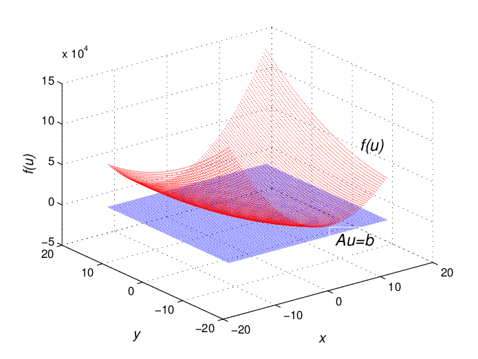
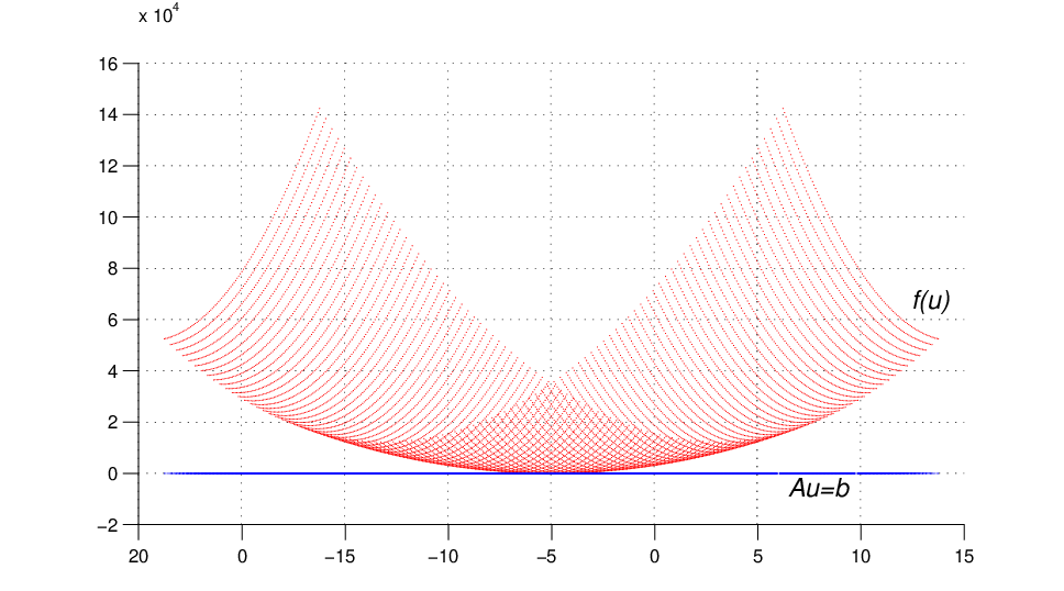
This example can be represented graphically as follows, clearly showing the constrained minimization and the uniqueness of the solution:
In the case of the minimization of , then the set
is
nonempty.
The vector belongs to
and therefore, . The same answer would be given using the
algorithm proposed by Stoika et al [18].
4 Conclusions
In this work we extend a minimization result concerning non singular quadratic forms using the Moore-Penrose inverse, to infinite dimensional Hilbert spaces. In addition, in the case of a singular quadratic form the minimization takes place for all its non zero values. This proposed Constrained minimization method has the advantage of a unique solution and is easy to implement. Practical importance of this result can be in numerous applications such as filter design, spectral analysis, direction finding etc. In many of these cases the quadratic form may be very close to, or even exactly singular, and therefore the knowledge of the non zero part of the solution may be of importance.
References
- [1] A. Ben-Israel and T. N. E. Grenville (2002). Generalized Inverses: Theory and Applications, Springer- Verlag, Berlin.
- [2] A. Ben-Israel, A. Charnes (1963). Generalized Inverses and the Bott-Duffin Network Analysis, J. Math. Analysis and Appl., (7), pp. 428- 435.
- [3] R. Bouldin ( 1973). The pseudo-inverse of a product, SIAM J. Appl. Math. 24 (4) pp. 489-495.
- [4] R. Bouldin ( 1973). The product of operators with closed range, Tohoku Math. J. 25 (4) pp. 359-363, .
- [5] M. Broom (1993). On the number of local maxima of a constrained quadratic form, Proc. Roy. Soc. London Ser. A 443 , no 1919, pp. 573- 584.
- [6] S. L. Campbell and C. D. Meyer (1979). Generalized inverses of Linear Transformations, Dover Publ. New York.
- [7] J. Conway (1985). A course in functional analysis, Springer Verlag New York.
- [8] D. Drivaliaris, S. Karanasios, D. Pappas (2008). Factorizations of EP operators, Linear Algebra Appl. 429 pp. 1555-1567.
- [9] C. W. Groetsch (1977). Generalized inverses of linear operators, Marcel Dekker Inc. New York.
- [10] A. Gorokhov, P. Stoica (1998). Generalized quadratic minimization and signal processing applications, EUSIPCO ’98, 9th European Sign. Proc. Conference, Rhodes, Greece .
- [11] S. Izumino(1982). The product of operators with closed range and an extension of the reverse order law, Tohoku Math. J. 34, 43–52.
- [12] S. Karanasios , D. Pappas (2006). Generalized inverses and special type operator Algebras, Facta Univ. Ser. Math. Inform., (21), pp. 41–48.
- [13] W. La Cruz (2009). Extension of the Barzilai- Borwein method for quadratic forms in finite Euclidean spaces. Numer. Funct. Anal. Optim. 30 (3- 4) pp. 306-321, .
- [14] D. Luenberger (1969). Optimization by Vector Space Methods, Wiley Publ. New York.
- [15] R. Manherz, S. Hakimi (1969). The Generalized Inverse in Network Analysis and Quadratic- Error Minimization Problems, IEEE Trans. Circuit Theory, vol. 16 (4), pp. 559- 562.
- [16] H. Markowitz (Mar. 1952). Portfolio Selection. J. Finance, 7, No.1. , pp. 77-91.
- [17] H. Markowitz (1959). Portfolio Selection. Cowles Foundation Monograph N.16. New York John Wiley and Sons Inc.
- [18] P. Stoika, A. Jakobsson, J. Li (1996). Matrix Optimization Result with DSP Applications. Dig. Signal Proc., A review Journal, 6 , pp. 195- 201.