A message passing approach for general epidemic models
Abstract
In most models of the spread of disease over contact networks it is assumed that the probabilities per unit time of disease transmission and recovery from disease are constant, implying exponential distributions of the time intervals for transmission and recovery. Time intervals for real diseases, however, have distributions that in most cases are far from exponential, which leads to disagreements, both qualitative and quantitative, with the models. In this paper, we study a generalized version of the SIR (susceptible-infected-recovered) model of epidemic disease that allows for arbitrary distributions of transmission and recovery times. Standard differential equation approaches cannot be used for this generalized model, but we show that the problem can be reformulated as a time-dependent message passing calculation on the appropriate contact network. The calculation is exact on trees (i.e., loopless networks) or locally tree-like networks (such as random graphs) in the large system size limit. On non-tree-like networks we show that the calculation gives a rigorous bound on the size of disease outbreaks. We demonstrate the method with applications to two specific models and the results compare favorably with numerical simulations.
I Introduction
The mathematical modeling of infectious disease outbreaks in human populations has a long history, stretching back to the pioneering work of Lowell Reed, Anderson McKendrick, and others in the early twentieth century [1]. The standard analytic approach involves dividing the modeled population into classes or compartments according to their status with respect to the disease of interest—uninfected but susceptible, infected, recovered, and so forth—and then writing differential equations to describe the mass flow of individuals between compartments according to the dynamics of the infection process [1, 2].
Such compartmental models have proven flexible, tractable, and highly informative as a general guide to the population-level behavior of diseases, but they also suffer from a number of serious deficiencies, of which two are particularly significant. The first, which has attracted a lot of recent attention in the literature, is the assumption of random mixing. In order to write differential equations for flows between compartments, we must make a fully mixed or mass-action approximation whereby we assume that the probability of disease-causing contact with any member of a particular compartment is the same. In real life this is far from true—most people have high probability of contact with only that small fraction of the population they rub shoulders with regularly, and a very small chance of contact with everyone else. The incorporation of more realistic mixing patterns into epidemiological modeling has given rise to the field of network epidemiology, in which contacts are modeled as a network, either static [3, 4, 5, 6, 7, 8, 9] or dynamic [10, 11, 12], and the structure of the network can have a profound impact on the spread of the disease [13, 14, 15, 16].
In this paper, however, we focus on a different shortcoming of compartmental models, one that has by comparison received little attention, but which is at least as important as the mass-action approximation. In order to write down the differential equations of a compartmental disease model, one must make the assumption that movement between compartments takes place at a stochastically constant rate. In modeling a disease from which most victims recover, for instance, one typically assumes that an infected individual has a constant probability per unit time of recovery. While being a useful assumption from a mathematical point of view, however, this behavior is very far from that of most real diseases. The assumption of constant probability of recovery implies an exponential distribution of times for which individuals remain infected, so that the most probable duration of infection is zero, and probability decreases uniformly with time. In reality, most diseases show a roughly constant duration of infection—a week, say, or a month—with relatively small fluctuations from person to person, so that the distribution of durations has a sharp peak about the average value and is highly nonexponential. Such nonexponential distributions are known to have a substantial effect, both qualitative and quantitative, on the shape of epidemics [17, 18, 19, 20, 21].
If one is willing to make the mass-action approximation, then nonexponential behavior can be incorporated into epidemic models by reformulating the theory in terms of integro-differential equations [22, 23]. If, however, one wishes also to retain the advances of network epidemiology in representing nonrandom contact patterns, then even this approach does not work and a new method of solution is necessary. In this paper we demonstrate that in the latter case the calculations can be reformulated in the language of message passing algorithms of the kind known as belief propagation or sum-product methods. In addition to providing exact solutions for the dynamics of quite general epidemic models on large classes of networks, the message passing formulation also leads to a number of other results concerning network epidemiology, including a rigorous upper bound on the size of disease outbreaks, results for late-time behavior, and results for the average behavior of epidemics in random network ensembles.
II A message passing formulation of epidemics
We begin by defining the problem. We consider the simplest nontrivial model of epidemic disease, the SIR model, in which an individual can be in one of three disease states, susceptible, infected, or recovered. We will assume an initial condition for the epidemic in which each vertex is susceptible with independent probability and infected otherwise.
We assume that disease transmission is taking place on a given contact network, meaning that disease can only be transmitted between individuals who are directly connected by an edge in that network. We also generalize the model to allow for nonexponential distributions of the times at which transitions between these states occur, i.e., the times at which infection and recovery occur. To be completely general, let us define to be the probability that an individual infected with the disease of interest first makes contact sufficient to transmit the disease to a particular network neighbor at a time between and after their infection. Similarly let us define to be the probability that an individual infected with the disease recovers from it at a time between and after infection.
An infected individual can only transmit the disease to a susceptible neighbor if they are still infected at the time of contact, and hence the probability that transmission actually occurs between and after infection is equal to the probability times the probability that the individual has not yet recovered. Let us denote this overall probability of transmission by :
| (1) |
Note that this function, unlike and does not integrate to unity. Rather, it integrates to the total probability that a vertex transmits the disease to its neighbor before it recovers, a probability referred to elsewhere variously as the transmissibility or infectivity of the disease.
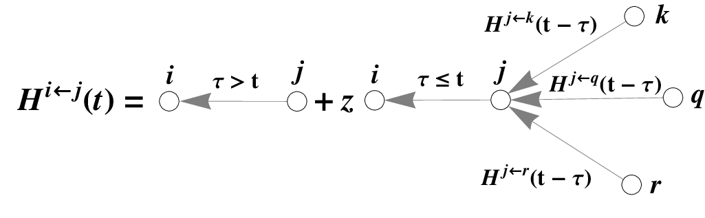
The fundamental quantity appearing in our message passing formulation of disease transmission—the “message” that is passed among network vertices in the calculation—is the probability, which we denote , that a vertex has not passed the disease to neighboring vertex by absolute time . (Without loss of generality, we will assume the epidemic to begin at absolute time .) An especially simple case of our approach arises when the network of interest takes the form of a tree, i.e., a network having no loops. In this case, the failure of vertex to pass the disease to vertex before time can occur in either of two ways, as illustrated in Fig. 1. First, it may be that, if and when vertex contracts the disease, it fails to transmit it to within an interval from infection, in which case clearly does not contract the disease before absolute time . The probability of this occurrence is .
The second possibility is that is scheduled to transmit the disease within time of contracting it, but that itself got the disease (from one of its other neighbors) too late for that transmission to occur before absolute time , or indeed never got the disease at all. If transmits the disease at time after contracting it, but fails to contract the disease before time then does not receive the disease before time . The probability that does not contract the disease before is , where the leading factor of represents the probability that was not one of those vertices initially infected with the disease at . The notation denotes the set of neighbors of vertex , excluding vertex . Now integrating over , we find the total probability that fails to transmit the disease before to be .
Putting the two contributions to together and writing we arrive at the message passing equation
| (2) |
For the special case of a network taking the form of a tree, this equation gives us, at least in principle, a complete solution for the probabilities for all and arbitrary .
Normally, however, is not the quantity of epidemiological interest. More commonly one wants to know things such as the fraction of the population that will be in the various disease states at different times, or more generally the probability that a particular individual will be in each disease state. Let us define to be 1 if individual is susceptible at time and 0 otherwise, and similarly define and for the infected and recovered states. Then denotes the probability that vertex is susceptible at time . For the sake of economy we will also write this probability more briefly simply as . For to be susceptible at time we require (a) that is not one of the vertices initially infected at , which happens with probability , and (b) that not receive the infection from any of its neighbors before time . Thus can be expressed quite simply as
| (3) |
Once we have , however, one can also immediately calculate and . Note that the rate at which increases is equal to the rate at which decreases—since all individuals moving out of the susceptible state must move into the infected state—minus the rate at which recovers. The recovery rate has two contributions: the probability that was infected at time times the rate of recovery a time later, and the probability that was infected at some later time (which is simply ) times the rate of recovery a time later. This allows us to write a rate equation for thus:
| (4) |
By integrating this equation we can calculate for any , and then we can calculate from the knowledge that the probabilities of the three states must sum to one:
| (5) |
Between them, Eqs. (2) to (5) now give us a complete solution for the three probabilities, for arbitrary (including nonexponential) distributions of infection and recovery times.
III Message passing on non-tree networks
The developments of the previous section give us a solution for the SIR model in the case where the network of interest has no loops, but almost all real-world networks have loops, and usually many of them. It is known that message passing methods, while not exact on non-tree networks can still give good approximate answers in some cases. In the present case, however, we can go further than such qualitative statements and show that our message passing calculation provides a rigorous upper bound to the number of infected individuals on networks that contain loops. To prove this result, consider the following alternative formulation of the epidemic process.
In the generalized SIR model discussed here, evolution of the disease involves infected individuals spreading infection to their susceptible neighbors at times after infection drawn from the distribution and recovering at times after infection drawn from . There is, however, no requirement that we draw these times at the moment of infection. We can if we wish draw them ahead of time, before executing the steps of the model. That is, we can for each vertex in the network draw a time from the distribution and associate it with that vertex. When vertex becomes infected, we look up the value of which tells us the interval of time before recovers. For the edges the situation is only a little more complicated. We replace each undirected edge in the network with two directed edges pointing in opposite directions, to represent the act of disease transmission in either direction between the two relevant vertices. Then for each directed edge we draw a time from the distribution to represent the time after infection of at which contact is made with . If this time falls before the recovery of , i.e., if , then transmission will take place if is ever infected, and will occur an interval after infection. If, however, recovers first, i.e., if , then no transmission takes place, which we can, if we wish, represent mathematically by setting .
The end result is a directed “transmission network” in which the edges represent possible transmission events and the values on the edges represent the time delay between arrival of the infection at (if that ever happens) and arrival of the infection at .
In terms of this network it is now quite simple to write down the probability that vertex is susceptible at time . In order to be susceptible we require (a) that was not infected at time , which happens with probability , and (b) that there exists no path from any vertex to vertex such that vertex was infected at time and the sum of the time delays along the path is less than .
An alternative way of thinking about this second condition is to consider the neighborhood of radius about vertex , meaning the set of vertices a distance or less from , where distance is measured in terms of the sum of the values along the path—the shortest weighted distance in the language of graph theory. If any of the vertices in this neighborhood is infected at time zero then vertex will not be susceptible at time . Let us suppose that there are vertices in the neighborhood, excluding vertex itself. Then the probability that is susceptible—for this particular choice of the and —is . We are interested, however, in the probability averaged over all values of the and , which is
| (6) |
where the angle brackets denote the average over the ensemble of values of and .
This equation is correct and exact in all cases. To relate it to our previous message passing approach and understand how the calculation proceeds on networks with loops, consider the alternative set of vertex counts , which are the numbers of vertices whose distance to is or less, but now with the restriction that the penultimate vertex along the path to must be vertex . For reasons that will shortly become clear, we also forbid paths that pass through vertex more than once. That is, there may be a path of length or less that first passes through to reach and then returns to , but such paths are disallowed. In practice, a simple way to enforce this constraint is to remove from the network all directed edges outgoing from vertex . In this case, vertex is said to be a cavity vertex or in the cavity state.

We now observe that, as illustrated in Fig. 2, the sum of over all neighbors is always at least as great as :
| (7) |
where the inequality becomes an exact equality if the network is a tree. (It is in order to ensure this equality that we exclude paths that pass through twice.) Then and
| (8) |
We now apply a version of the Chebyshev integral inequality, proved in the appendix, that for any set of non-negative functions that are monotone increasing or decreasing in every argument, says
| (9) |
where the average is over any distribution of independent variables . Applied to Eq. (8), this inequality tells us that
| (10) |
where we have defined
| (11) |
This quantity is the average probability that at time the infection has not been passed to vertex via neighbor (again excluding cases where the infection passes through twice). It plays the same role as the corresponding quantity in Eq. (3) for the case of a tree, and we can evaluate it in an analogous way. As before we split into two parts. The first is the probability that, even if is infected, it does not transmit the disease to within time of infection. This probability, as before, is , where is defined by Eq. (1).
The second part is the probability that is scheduled to transmit the disease within time of contracting it, but that itself gets the disease too late for the transmission to occur before absolute time (or never gets the disease at all). For transmission before time vertex needs to contract the disease before and the probability that this does not happen is , where it is now important that is in the cavity state, so as to disallow paths for infection that pass through itself. Then the probability that fails to transmit the disease before time is .
The probability we can calculate from the appropriate analog of Eq. (10) but with both and in the cavity state, i.e., with their outgoing edges deleted. But consider now adding back in all the edges leading from except the one to . In doing so we only add paths to the network and hence potentially increase the size of the neighborhood of vertex but never decrease it. This implies that we only decrease , so that
| (12) |
where we have used Eq. (10). Combining our two contributions to and writing , we now find that
| (13) |
This result is very similar to the message passing equality of Eq. (2), but it is an inequality, and hence cannot be directly employed to calculate properties of the epidemic. Let us, however, define a different function by the equation
| (14) |
which is an equality and so can be used to calculate , for instance by iteration starting from a suitable initial value . Suppose we choose as our initial value for all and , so that, from Eq. (13), we have
| (15) |
(Of course we don’t know the value of , but suppose for the moment that we do.) Then, performing one step of the iteration, we arrive at a new value thus:
| (16) |
where we have used Eq. (15). But note that, since for all , Eq. (16) also implies that
| (17) |
and hence from Eq. (16)
| (18) |
which is the equivalent of Eq. (15) for . Now we can repeat the same argument to show that for a general step of the iteration we must have
| (19) |
In the limit , the iteration must converge, since is bounded below by , and hence in this limit we get a solution to Eq. (14) that satisfies
| (20) |
for all and .
Now, making use of Eq. (10), we have
| (21) |
Thus Eq. (14) allows us to calculate a rigorous lower bound on the probability that any vertex is in the susceptible state. Notice that Eq. (14) is the same as the equation for in the tree case, Eq. (2), but is perfectly well defined for any network, tree or otherwise.
Our lower bound on also gives us upper bounds on and , both of which are trivially less than , as well as an upper bound on the sum , which is the total probability that has ever caught the disease. Hence our message passing calculation can in this case give us an upper bound on the number of individuals infected by an epidemic, a result of possible value—a guarantee that infection will not rise above a certain level could be used as a quality function to quantify the efficacy of proposed vaccination campaigns or other public health interventions.
Employing Eqs. (14) and (21) in a message passing algorithm would involve propagating messages that take the form of functions of time. On a tree, one would start with the leaves of the tree, for which Eq. (14) is trivial, and work inwards through the network until the functions on all edges have been evaluated. On a non-tree network, the calculation is more complicated because one does not in general know any of the to begin with, so one would have to make an initial guess and then iterate Eq. (14) repeatedly to reach convergence. for all and is a suitable starting condition, but the iteration itself can in practice be time-consuming and the calculation may not be tractable. Even if it is tractable, it almost certainly demands more effort than simply simulating the spread of an epidemic on the network of interest. There are some choices of the distributions for which the equations simplify and are more tractable—we examine two in Section V. Alternatively, one may be able to make useful approximations in some cases. For instance, if is sharply peaked close to , as it is for many real diseases, then it may be reasonable to approximate in Eq. (14) by its value at . Then (14) becomes
| (22) |
where . Hence the values of at different times decouple and the equations can be solved by a simple scalar iteration—no integrals need be performed. Although efficient, however, this approximation is usually only a good one in regions where is relatively constant over the timescales typical of the disease progression represented by , which means early and late times, but not in the crucial intermediate interval where most of the interesting behavior falls.
Even in cases where the message passing equations are not a practical calculational tool, however, they can still be useful. In particular, they can tell us about the late-time limit of epidemics, including important quantities such as the total number of people infected by the disease, and they allow us to calculate epidemic outcomes averaged over ensembles of networks such as the widely-studied configuration model. We look at these two applications now in turn.
IV Late-time behavior
Taking the limit in Eq. (14), we get
| (23) |
where we have assumed that is suitably small for large values of its argument. Writing for short and defining , which is the total probability of transmission occurring between two vertices connected by an edge, we then find that
| (24) |
This again takes the form of a message passing calculation, but now the messages passed are simple numbers, and hence the calculation can be performed quickly, even on networks that are not trees. Then the probability that a vertex is susceptible in the limit of late times satisfies
| (25) |
In the limit of late times there are no infected individuals—all have either recovered or never got sick in the first place—so . Thus this calculation gives us an upper bound on the probability that any given individual ever contracts the disease or, if we sum over all vertices, an upper bound on the size of the disease outbreak.
As has been discussed previously [24, 25, 26, 27], the late-time limit of the SIR model is related to a correlated bond percolation process on the corresponding directed transmission network, the correlations arising because of variation in the time an individual takes to recover: if an individual recovers quickly then the probability of transmission of the disease to any of its neighbors is small; if it takes a long time to recover the probability is correspondingly larger. Equations (24) and (25) can be considered to define a message passing algorithm for solving precisely this bond percolation problem on a general network. In this context, is a generating function in for the number of vertices in the percolation cluster of vertex that are reachable via vertex , and is a generating function for the overall sizes of the clusters. In recent unpublished work, Shiraki and Kabashima [28] have given a message passing method for calculating percolation cluster sizes on trees and locally-tree-like networks, which is equivalent to the method reported here for the special case of a tree.
V Epidemics on configuration model networks
Our method can also be used to calculate average probabilities of infection for ensemble models of networks. It is common in the study of processes on networks to look at not the behavior on a single network, but the average behavior in an ensemble model defined as a probability distribution over possible networks. The message passing formalism developed here allows one to calculate such average behaviors easily. We demonstrate this type of calculation using the configuration model, which is probably the most widely studied ensemble model of a network [29, 30].
In the configuration model one fixes the degree distribution of the network—meaning the fractions of vertices with each possible degree —but in other respects connects vertices at random. Thus in calculating the behavior of an epidemic on the configuration model there are two sources of randomness to average over. The first is the randomness in the dynamics of the disease, which is already built into our message passing formalism. The second is the randomness of the graph ensemble.
Consider the average over the graph ensemble and consider an edge attached to vertex . In different networks of the ensemble this edge will be attached to different vertices at its other end and hence a different message will be transmitted down the edge. The ensemble average probability that vertex has not yet been infected along the edge by time is equal to the average of these messages over the set of networks. But, since every edge plays an identical role in the configuration model ensemble, the average message is the same for all edges and hence we need calculate only one message to solve for the average behavior of the model. Let us denote this average message by .
To calculate the average message, we need to average Eq. (2) (or its equivalent, Eq. (14) for non-tree networks), which requires us to average the product on the right-hand side of the equation. The average of such a product is not in general equal to the product of the average message, which potentially makes the calculation more complicated. However, in the limit of large network size, configuration model networks have the crucial property of being locally tree-like, with the shortest cycles in the network being of length and hence diverging as . This means that the messages a vertex receives along each of its incident edges are independent in the large- limit—in essence, we assume that correlations along a cycle of diverging length are irrelevant in the large size limit. In this case, the average of the product of messages received by a vertex is equal to the product of the average.
Averaging Eq. (2) over the ensemble and allowing for the fact that all messages are the same, the product in the equation now becomes simply a power , where is the so-called excess degree of , i.e., its degree minus the edge between and , which has been removed because is in the cavity state. The excess degree is distributed according to the excess degree distribution [30] and, averaging over this distribution, we find
| (26) |
where is the probability generating function for the excess degree distribution.
Similarly, from Eq. (3), the probability that a vertex of (ordinary) degree is susceptible at time is and the average probability of being susceptible is
| (27) |
where is the generating function for the ordinary degree distribution .
Again we can study the late-time behavior by letting and writing to give
| (28) |
and
| (29) |
where . These two equations are precisely the standard equations for bond percolation on the configuration model [31] and highlight again the connection between the SIR model and percolation theory. The message can be regarded as a generating function in for the distribution of numbers of vertices reachable along an edge in bond percolation and is a generating function for the sizes of clusters.

VI Examples
As a first example of the application of our formalism, consider what happens when the distributions and take the standard exponential form, corresponding to stochastically constant probabilities of infection with and recovery from disease. Specifically, we assume that and , where and are the rates of infection and recovery. Then and, making the substitution , Eq. (26) becomes
| (30) |
Differentiating with respect to , we then find that satisfies
| (31) |
with the initial condition . This differential equation has the solution
| (32) |
And once we have we can use Eq. (27) to calculate and subsequently and . In Fig. 3 (top two frames) we show the form of the resulting solution for the particular choice of a Poisson degree distribution, along with the results of numerical simulations of epidemics spreading on the same networks. As the figure shows, the analytic and numerical approaches agree well, and take the familiar form of an SIR outbreak with a brief peak in the number of infected individuals followed by a sharp decline and corresponding rise in the number of recovered individuals.
But now consider a second choice that is quite different but perhaps more realistic. In this case we assume that individuals once infected do not become infectious immediately, passing through a latent period before developing a transmissible infection, and also that infected individuals do not start recovering from disease immediately upon infection as in the exponential model, but remain infected for a certain length of time then recover. A simple choice displaying these two behaviors is the “top hat” function
| (33) |
with , where is the Heaviside step function. In this expression is the time at which the infected individual becomes infectious, is the time at which they recover, and , as before, is the total probability of transmission.
Inserting this form into Eq. (26) and again differentiating gives
| (34) |
where again . The lower two panels of Fig. 3 show the solution of this equation for the same Poisson degree distribution as previously, and , , and chosen so as to give the same mean time of transmission and total transmission probability as in the exponential case. Fixing the total transmission probability to be the same also fixes the long-time behavior to be the same, as can be seen in the figure.
The two calculations—exponential and “top hat” versions of —nonetheless give quite different results. The epidemic peaks around the same time in each (about in the plots), but more individuals are infected at any time in the exponential case and the epidemic lasts longer. Furthermore, the top hat case shows distinctive waves of infection, of period roughly equal to , separated by intervals of comparatively lower disease activity. These waves are caused by the appearance of distinct “generations” in the spread of the disease as the first round of disease carriers passes infection to the second, who some time later pass it to the third, and so on. Such waves of infection are observed in many real-world diseases but are absent from models using a conventional exponential distribution of infection times (although they can be represented in a crude fashion by introducing additional disease states, as in the so-called SEIR model).
For other choices of degree distribution, including power-law, uniform, and exponential distributions, the predictions are qualitatively similar by and large, and agree similarly well with simulation results. The shapes of the curves are, however, significantly altered by different choices of the parameters and in the top hat case: as the values of and become better separated the waves of infection become blurred and ultimately impossible to distinguish. Conversely, the waves become more pronounced if and are chosen closer to one another.
VII Conclusions
In this paper, we have studied the SIR model of epidemic disease on a contact network, in a generalized form that allows for non-constant probabilities of infection and recovery, by contrast with conventional SIR calculations. Abandoning constant probabilities obliges us also to abandon the traditional differential equation approach to solving the model, but we have shown that the problem can be reformulated instead in the language of message passing. We have given a message passing calculation that is exact on networks that take the form of trees (or are locally tree-like, as in random graphs) and provides a rigorous bound on the probabilities of disease states on non-tree-like networks.
We have demonstrated the application of our approach to the calculation of the late-time behavior of the generalized SIR model and to the calculation of average properties of the model within the random graph ensemble known as the configuration model. One could in principle extend the calculations to other random graph ensembles, such as random graphs with degree correlations [32] or random graphs with clustering [33], or to calculations on single networks (i.e., not ensembles).
The approach taken here can be applied to other dynamical models on networks, such as the SI or SEIR models, again yielding exact results on trees or tree-like networks and rigorous bounds in the non-tree case, and it is possible the approach could also be applied to threshold models [34]. At the moment, it’s unclear whether models such as the SIS model in which vertices can return to past states can be tackled in the message passing framework. The developments for the SIR model relied on our having an exact message passing solution on a tree. We have not yet been able to find a similar solution for the SIS model and so the development of a message passing method for this model remains an open problem.
Acknowledgements.
The authors thank Lenka Zdeborova for useful conversations. This work was funded in part by the National Science Foundation under grant DMS–0804778 and by the James S. McDonnell Foundation.*
Appendix A Chebyshev Integral Inequality
Let be a set of non-negative functions that are monotone decreasing or increasing in each of their real-valued arguments for fixed values of the other arguments. (They can be increasing in one argument and decreasing in another.) Then it can be proved that
| (35) |
where the average is over any distribution of the independent variables . The proof is as follows.
Let denote the partial average
| (36) |
which is a function of the remaining arguments to . Then consider the following product for arbitrary and
| (37) |
Because the functions are non-negative and monotonic in their first argument, the factors in brackets are either both positive or both negative and hence the entire expression is non-negative for any and . Now let and be independent random variables, both with the same distribution as and let us average (37) over and . After rearranging we find that
| (38) |
The same argument can now be applied to the remaining functions in turn, to demonstrate that
| (39) |
and the equivalent result naturally holds for averages over any of the variables:
| (40) |
The remainder of the proof proceeds by induction. Assume that
| (41) |
for . Averaging both sides over one additional variable gives
| (42) |
But is itself a set of monotone non-negative functions of the variables . Applying Eq. (40) to this set, we then find that
| (43) |
Applying induction and using Eq. (39) as the base case, the result is now established.
References
- [1] R. M. Anderson and R. M. May, Infectious Diseases of Humans (Oxford University Press, Oxford, 1991).
- [2] H. W. Hethcote, SIAM Review 42, 599 (2000).
- [3] R. Pastor-Satorras and A. Vespignani, Phys. Rev. Lett. 86, 3200 (2001a).
- [4] R. Pastor-Satorras and A. Vespignani, Phys. Rev. E 63, 066117 (2001b).
- [5] Y. Moreno, R. Pastor-Satorras, and A. Vespignani, Eur. Phys. J. B 26, 521 (2002).
- [6] M. J. Keeling, D. Rand, and A. Morris, Proc. Biol. Sci. 264, 1149 (1997).
- [7] K. T. Eames and M. J. Keeling, Proc. Natl. Acad. Sci. USA 99, 13330 (2002).
- [8] K. J. Sharkey, Journal of Mathematical Biology 57, 311 (2008).
- [9] E. Volz, Journal of Mathematical Biology 56, 293 (2008).
- [10] E. Volz and L. A. Meyers, Proc. Biol. Sci. 274, 2925 (2007).
- [11] T. Gross, C. J. D. D’Lima, and B. Blasius, Phys. Rev. Lett. 96, 208701 (2006).
- [12] J. M. Read, K. T. Eames, and W. J. Edmunds, Journal of The Royal Society Interface 5, 1001 (2008).
- [13] M. J. Keeling and K. T. Eames, J. R. Soc. Interface 2, 295 (2005).
- [14] M. Barthélemy, A. Barrat, R. Pastor-Satorras, and A. Vespignani, Journal of Theoretical Biology 235, 275 (2005).
- [15] P. Trapman, Theoretical Population Biology 71, 160 (2007).
- [16] S. Bansal, B. T. Grenfell, and L. A. Meyers, J. R. Soc. Interface 4, 879 (2007).
- [17] A. L. Lloyd, Theoretical Population Biology 60, 59 (2001a).
- [18] A. L. Lloyd, Proceedings of the Royal Society of London. Series B: Biological Sciences 268, 985 (2001b).
- [19] H. J. Wearing, P. Rohani, and M. J. Keeling, PLoS Med 2, e174 (2005).
- [20] A. Vazquez, B. Rácz, A. Lukács, and A.-L. Barabási, Physical Review Letters 98, 158702 (2007).
- [21] J. L. Iribarren and E. Moro, Phys. Rev. Lett. 103, 038702 (2009).
- [22] H. W. Hethcote and D. W. Tudor, J. Math. Biol. 9, 37 (1980).
- [23] M. J. Keeling and B. T. Grenfell, Science 275, 65 (1997).
- [24] M. E. J. Newman, Phys. Rev. E 66, 016128 (2002a).
- [25] J. C. Miller, Phys. Rev. E 76, 010101 (2007).
- [26] E. Kenah and J. M. Robins, Phys. Rev. E 76, 036113 (2007).
- [27] J. C. Miller, J. Appl. Prob. 45, 498 (2008).
- [28] Y. Shiraki and Y. Kabashima, Preprint arXiv:1002.4938v1 (2010).
- [29] M. Molloy and B. Reed, Random Structures and Algorithms 6, 161 (1995).
- [30] M. E. J. Newman, S. H. Strogatz, and D. J. Watts, Phys. Rev. E 64, 026118 (2001).
- [31] D. S. Callaway, M. E. J. Newman, S. H. Strogatz, and D. J. Watts, Phys. Rev. Lett. 85, 5468 (2000).
- [32] M. E. J. Newman, Phys. Rev. Lett. 89, 208701 (2002b).
- [33] M. E. J. Newman, Phys. Rev. Lett. 103, 058701 (2009).
- [34] P. S. Dodds and D. J. Watts, Phys. Rev. Lett. 92, 218701 (2004).