The momentum analyticity of two point correlators from perturbation theory and AdS/CFT

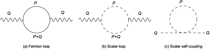
To the zeroth order of the Yang-Mills coupling, this correlator is given by the one-loop diagram of Fig.1. We have

where $F_{f}(q)$ accounts for the contribution of each Weyl fermion of unit charge and $F_{b}(q)$ accounts for the contribution of each complex scalar of unit charge. It follows from the Feynman rule at nonzero temperature that

with $P=(\nu_{n},\vec{p})$ and

where Matsubara frequencies $\nu_{n}=2\pi T(n+\frac{1}{2})$ and $\omega_{n}=2\pi Tn$. The dimensional regularization is applied with $D\to 4^{-}$ and $\mu$ an energy scale to compensate the dimensionality. Following the standard procedure in textbooks, we obtain that

and

with $\gamma_{E}=0.5772...$ the Euler constant. To explore the analyticity for a complex $q$, it is more convenient to perform the integrations (4) and (5) differently. Upon Feynman parametrization of the integrand according to

we find that

and

It follows that $F_{f}(q)$ and $F_{b}(q)$ are analytic on the complex $q$-plane cut along the imaginary axis. The discontinuities acrossing the cut are given by

and

where $N_{f}\geq 0$ and $N_{b}\geq 0$ are the maximum integers such that $\kappa^{2}\geq 4\nu_{N_{f}}^{2}$ and $\kappa^{2}\geq 4\omega_{N_{b}}^{2}$. The same analyticity including the discontinuities can be extracted from (6) and (7) with a careful treatment of the logarithm of the integrands. See appendix A for details. We notice that ${\rm Im}F_{f,b}(i\kappa+0^{+})>0(<0)$ for $\kappa>0(<0)$, consistent with the identity

for an analytic function that is real for real $q$. Substituting (6) and (7) into (3) we obtain that

where we have introduced a UV cutoff length $l$ via

The discontinuity across the cut along the imaginary axis is given by

The above analyticity on the momentum plane is generic to a Feynman diagram of a two point Green’s function consisting of an arbitrary finite number of loops. For a self-energy diagram of $I$ internal lines and $L$ loops, we have

where $K_{i}=(\omega_{i},\vec{k}_{i})$ is the four momentum of the i-th internal line and $N(P,Q)$ is a polynomial of loop momenta $P_{l}=(\nu_{l},\vec{p}_{l})$’s and $Q=(q_{0},0,0,q)$. Introducing Feynman parameters, we find that

where

with $M_{ll^{\prime}}$, $u_{l}$ and $v$ functions of the Feynman parameters $x$’s. $M_{ll^{\prime}}$ forms a $L\times L$ symmetric and positive matrix. Upon an orthogonal transformation and a translation,

with all $\lambda_{l}$’s positive. Regarding the self-energy part as a DC circuit with the i-th internal line carrying a resistance of $x_{i}$, the function ${\cal R}$ equals to the total resistance between the two terminals of the external lines. We obtain that

which is analytic throughout the complex $q$-plane except a cut along the imaginary axis. Note that we did not assume the static limit in the analysis and the result is not restricted to the Coulomb component of the photon self energy. While the discontinuity acrossing the cut may be subject to the UV divergence in general, it should be finite for $N=4$ SYM. On the other hand, the infrared divergence cannot be removed perturbatively beyond certain orders, leaving rooms for nonperturbative modifications of the analyticity.

The location of the singularity is actually dictated by a general principle. The path integral of a relativistic thermal field theory at zero chemical potential reads

where $\Phi$ is the collection of the field variables and ${\cal L}_{E}$ is the Lagrangian density with a Euclidean time, which is of $O(4)$ invariance (For a gauge theory, manifest invariance can be implemented in the covariant gauge). The field theory at nonzero temperature $T=1/\beta$ is formulated on $R^{3}$. Switching the role of the Euclidean time $\tau$ and the spatial coordinate $x_{3}$, the same path integral describes a Euclidean field theory at zero temperature formulated on $S^{1}\times R^{2}$ with the same Lagrangian density, described by the partition function

The original complex momentum plane associated to the partition function $Z$ becomes the complex energy plane associated to the partition function ${\cal Z}$ with the positive imaginary axis of the former corresponding to the positive real axis of the latter. To see this mapping clearly, we notice that the spatial coordinate $x_{3}$ in $Z$ goes to the Euclidean time $\tau$ of ${\cal Z}$, which is related to the Minkowski time via $\tau=it$. Accordingly, the spatial momentum $q$ associated to $Z$ becomes the negative Euclidean energy $\omega$ associated to ${\cal Z}$ so that $e^{iqx_{3}}\to e^{-i\omega\tau}$ and $\omega$ is related to the Minkowski energy via $\omega=-iE$. It follows then that the spatial momentum $q$ of $Z$ maps to the Minkowski energy $E$ of ${\cal Z}$ according to $q\to iE$. The unitarity of the field theory specified by ${\cal Z}$ dictates singularities along the real axis of the energy plane only, which corresponds to the imaginary axis of the momentum plane of the original thermal field theory. The spectral representation of the self energy function implies that its imaginary part is negative when approaching the cut along the positive real axis from below and the residues of its poles are all positive along the positive real axis. The signs of RHS of (11) and (12) as well as the residues of the asymptotic poles discussed in the next section confirm the above statement.

It follows from the recipe just stated that the Coulomb component of the $R$-photon self energy is given by[16]

where $A_{0}(u|q)$ solves the equation

with $\hat{q}=q/(2\pi T)$. The indexes of this equation at the canonical singularity $u=1$ are 0 and 1, which give rise to two linearly independent behaviors as $u\to 0$,

or

The second solution, eq.(35) will make the action $S_{\rm sugr}$ diverge and should be discarded and the eq.(34) generates a power series power series solution

where the coefficients $a_{n}(q)$ satisfy the recursion relation

with $a_{0}(q)=1$. Notice that the coefficients are all polynomials in $q^{2}$ and is therefore analytic everywhere on the complex $q$-plane. The indexes at $u=0$ are also 0 and 1 so the series (36) converges for $0\leq 1-u\leq 1$ uniformly with respect to $q$. It follows from the Weierstrass theorem [18], that the sum $f(q)\equiv A_{0}(0|q)$ is an analytic function throughout the complex $q$-plane and is therefore an entire function.

Next, we consider the derivative $A_{0}^{\prime}(u|q)$. The indexes at $u=0$ implies two linearly independent behaviors there,

and

The solution (36) is a superposition of $A_{0}^{(1)}$ and $A_{0}^{(2)}$ and is dominated by $A_{0}^{(2)}$ as $u\to 0$, i.e.

and its derivative becomes logarithmically divergent at $u=0$. This is also consistent with the asymptotic behavior of the coefficients of (36) at large $n$,

where the overall factor ${\hat{q}}^{2}f(q)$ follows from (40). We find then

where

Each coefficient term of the infinite series above is analytic function of $q$ and the series converges unformily with respect to $q$. The same Weierstrass theorem applied to the infinite series of $A_{0}(0|q)$ implies that $g(q)$ is also an entire function of $q$. Substituting (42) and $A_{0}(\varepsilon|q)=f(q)+O(\varepsilon\ln\varepsilon)$ into (32) and dropping the terms that vanish in the limit $\varepsilon\to 0$, we obtain that

which is a meromorphic function of $q$.

The poles of $F(q)$ are determined by the zeros of $f(q)$, i.e.

It is easy to rule out the zeros off real and imaginary axes, where, ${\rm Im}q^{2}\neq 0$. Indeed, taking the imaginary part of the product of $A_{0}^{*}(u|q)$ and the equation (33) and integrating $u$ from 0 to 1 yield

If there were a complex $q^{2}$ satisfying (45), we would have

which requires that $A_{0}(u|q)\equiv 0$. It follows that there cannot be a nontrivial solution satisfying (45) with ${\rm Im}q^{2}\neq 0$. Turning to a real $q$, the equation (33) implies that the solution $A_{0}(u|q)$ is a convex(concave) function of $u$ if $A_{0}(u|q)>0(<0)$. Therefore starting with a nonzero $A_{0}(u|q)$ at $u\neq 0$ there is no way the solution cannot bent towards zero at $u=0$ and therefore there is no nontrivial solution satisfying (45) in this case either. The only location for the roots of $A_{0}(0|q)$ is the imaginary $q$-axis.

For large and imaginary $q$, i.e. $q=i\kappa$ with $\kappa>>T$, the WKB approximation of the appendix B yields

where

with $\hat{\kappa}\equiv\frac{\kappa}{2\pi T}$. Therefore the asymptotic locations of the poles are given by

and the number of them is infinite.

If follows from the AdS/CFT principle, the self-energy of the transverse $R$-photon is given by the coefficient of the term quadratic in $\vec{A}$ of the supergravity action (30). We have[16]

with $\varepsilon\to 0$, where ${\cal A}(u|q)$ solves the differential equation

Both indexes of (52) at $u=1$ are zero. Only the power series solution leaves the UV regularized action finite, which reads

where the coefficients are given recursively by

with $b_{0}=1$. The radius of convergence equal to one since none of the indexes, 0 and 1, at $u=0$ gives rise to divergent behavior there. It follows from the Weierstrauss theorem of the previous subsection that $G(q)$ is a meromorphic function of $q$.

Upon a transformation ${\cal A}=\frac{\psi}{\sqrt{1-u^{2}}}$, the eq.(52) becomes a one-dimensional Schroedinger equation

where the potential

and $\psi(u|q)=0$ is required to vanish faster than $\sqrt{1-u}$ as $u\to 1$. The same argument that rules out the poles of $F(q)$ with a nonzero ${\rm Im}q^{2}$ can be applied to the present case but the argument ruling out the poles on the real $q$ axis need to be modified because of the negative term of the potential. The attractiveness of the potential is maximized at $q=0$. If there were a nontrivial solution such that $\psi(0|q)=0$ ( i.e. ${\cal A}(0|q)=0)$ for a nonzero real $q$, the zero of ${\cal A}(u|q)$ at $u=0$ would shift towards $u=1$ when $q^{2}$ is reduced towards zero. Consequently, there would be a nontrivial solution at $q=0$, that vanishes at least once within the domain $u\in(0,1)$. This is, however, not the case. The exact solution of (52) for a finite action is ${\cal A}=1$. For a large and imaginary $q$, $q=i\kappa$, the WKB approximation yields

Therefore, the self-energy of a transverse $R$-photon is a meromorphic function of the momentum $q$ with infinite number of poles along the imaginary axis.

The shear component of the stress tensor correlator is extracted from the coefficients of the quadratic term in $h_{1}{}^{2}$, ${\cal C}_{1}{}^{2}{}_{1}{}^{2}(Q)$ of (30). It follows from the rotational symmetry about $x_{3}$-axis that $h_{1}{}^{2}=h_{2}{}^{1}$ does not couple with other components of the metric fluctuations and the quadratic action in $h_{1}{}^{2}$ is identical to that of a scalar field [16]. We have

where $\phi(u|q)$ solves the ordinary differential equation

which is the Fourier transform of the scalar Laplace equation the background metric (31). Between the two linearly independent solutions, only the power series solution

leaves the action (24) finite upon UV regularization, where the coefficients are given by the recursion relation

and are polynomials in $q^{2}$ again. The power series (60) is convergent at $u=0$. Making the transformation $\phi=\sqrt{\frac{u}{1-u^{2}}}\psi$, the equation (59) can be converted into an one-dimensional Schroedinger equation of zero energy in the potential

which is the least repulsive at $q=0$. The exact solutions of (59) at $q=0$ is $\phi(u|q)=1$. For $q=i\kappa$ with $\kappa>>T$, we find that

Therefore the arguments applied in the last subsection for the transverse $R$ photon self-energy implies that $\Pi(q)$ is a meromorphic function with an infinite number of poles along the imaginary axis of the $q$-plane, like the other two cases.

References

- [1] See e.g. C. Itzykson and J.-B. Zuber , Quantum Field Theory, Section 5.3, Dover Publications 2006
- [2] V. P. Silin, Zh. Eksp. Teor. Fiz. 38, 1577 (1960) [Sov. Phys. JETP 11, 1136 (1960)]; V. N. Tsytovich, Zh. Eksp. Teor. Fiz. 40, 1775 (1961) [Sov. Phys. JETP 13, 1249 (1961)]; O. K. Kalashnikov and V. V. Klimov, Yad. Fiz. 31, 1357 (1980).
- [3] H. A. Weldon, Phys. Rev. D 26, 1394 (1982).
- [4] R. Pisarski, Physica A 158, 246 (1989); Phys. Rev. Lett. 63, 1129 (1989)
- [5] J. Kapusta and T. Toimela Friedel oscillations in relativistic QED and QCD, Phys.Rev. D 37, 3731 (1988).
- [6] A. D. Linde, Phys. Lett. B 96, 289 (1980).
- [7] J. M. Maldacena, The large limit of superconformal field theories and supergravity, Adv. Theor. Math. Phys. 2, 231 (1998) [Int. J. Theor. Phys. 38, 1113 (1999)] [hep-th/9711200].
- [8] E. Witten, Anti-de Sitter space and holography, Adv. Theor. Math. Phys. 2, 253 (1998) [hep-th/9802150].
- [9] O. Aharony, S. S. Gubser, J. Maldacena, H. Ooguri and Y. Oz, Large N field theories, string theory and gravity Phys. Rept. 323, 183 (2000) [hep-th/9905111].
- [10] D. T. Son and A. O. Starinets, Viscosity, black holes and quantum field theory, Ann. Rev. Nucl. Part. Sci., 57, 95 (2007) [arXiv:0704.0240].
- [11] A. Núñez and A. O. Starinets AdS/CFT correspondence, quasinormal modes, and thermal correlators in N = 4 SYM, Phys.Rev. D 67,124013 (2003) [hep-th/030202].
- [12] Pavel K. Kovtun and A. O. Starinets Quasinormal modes and holography, [Phys.Rev. D 72, 086009 (2005)] [hep-th/0506184].
- [13] S. C. Huot, P. Kovtun, G. D. Moore, A. Starinets and L. G. Yaffe Photon and dilepton production in supersymmetric Yang-Mills plasma, JHEP 0612, 015 (2006) [hep-th/0607237].
- [14] M. Le Bellac, Thermal Field Theory(Cambridge Univ. Press, Cambridge, 1996)
- [15] D. Z. Freedman, S. D. Mathur, A. Matusis and L. Rastelli Correlation functions in the CFTd/AdSd+1 correspondence, Nucl.Phys. B 546, 96 (1999) [hep-th/9804058].
- [16] G. Policastro, D. T. Son and A. O. Starinets From AdS/CFT correspondence to hydrodynamics, JHEP 0209, 043 (2002) [hep-th/0205052].
- [17] The UV cutoff can also be implemented via a dimensional regulariztion, which amounts to write with .
- [18] E. C. Titchmarsh, The Theory of Functions(Oxford Univ. Press, 1939), Section 2.8.
- [19] H. Liu, D. Hou and J. R. Li Oscillatory Behavior of In-medium Interparticle Potential in Hot Gauge System with Scalar Bound States, Commun. Theo. Phys. 51, 1107(2009)[hep-ph/0703305]
- [20] Chengfu Mu and Pengfei Zhuang, Eur. Phys. J. C 58, 271 (2008) [arXiv:0803.0581].
- [21] J. Diaz Alonso, A. Pérez and H. Sivak,Linear response and Friedel oscillations of the pion field in relativistic nuclear matter Nucl. Phys. A505, 695 (1989)
- [22] J. Diaz Alonso, A. Pérez and H. Sivak Screening effects in Relativistic Models of Dense Matter at Finite Temperature Prog.Theor.Phys. 105, 961 (2001) [hep-ph/9803344]
- [23] J. Erlich, E. Katz, D. T. Son and M. A. Stephanov, QCD and a Holographic Model of Hadrons, Phys. Rev. Lett 95, 261602 (2005) [hep-ph/0501128]
- [24] V. P. Nair, Yang-Mills theory in (2+1) dimensions: a short review, Nucl. Phys. Proc. Suppl., 108, 195 (2002) [hep-th/0204063] and the references therein.
- [25] We thank V. P. Nair for pointing out that a glueball does not decay at large .