A model of fasciculation and sorting in mixed populations of axons

In our model, each growing axon is represented by a directed random walk in two spatial dimensions (Fig. 2$(a)$). The random walkers (representing the growth cones) are initiated at the epithelium ($y=0$, random even $x$) with a birth rate $\alpha$, and move towards the bulb (large $y$) with constant velocity $v_{y}=1$. In the case of multi-type systems, a type is assigned to each newly initiated random walker (specifically in the simulations of Sec. VIII, the type is decided randomly with equal probability for each of the two types). The trail generated by a random walker (growth cone) is regarded as an axon shaft. A forward moving directed random walker (growth cone) interacts with trails (axon shafts) of other walkers. In the numerical implementation on a tilted square lattice, at each time step the growth cone at ($x,y$) can move to ($x-1,y+1$) (left) or ($x+1,y+1$) (right). The probability $p_{\{L,R\}}$ to move left/right is evaluated based on the axon occupancies at the ($x\pm 1,y+1$) sites and their nearest neighbors ($x\pm 3,y+1$) (see Fig. 2$(a)$). At a given $y$, two axons are considered to be part of the same fascicle if they are not separated by any unoccupied sites (i.e., they are not separated by more than two lattice spacings).

We assume a short-range attractive interaction between each growth cone and the close-by axon shafts. The range of interaction (two lattice spacings in our model) corresponds biologically to the range of extension of sensory filopodia from the growth cone (of the order of $10\mu{\rm m}$). The attractive interaction is mediated by cell adhesion between the growth cone and the axon shafts. We assume that the interactions are additive and type-specific. For a given growth cone, the model assumes a weak nearest neighbor attraction $E_{o}<0$ if the neighboring axon shaft is of a different type and a stronger attraction $E_{h}\,(<E_{o})$ if the neighboring axon shaft is of the same type. In each time step, a growth cone at $(x,y)$ attempts a Monte Carlo move to the left $(x-1,y+1)$ and to the right $(x+1,y+1)$ with probabilities $1/2$. The moves are accepted with probabilities

(or $p_{R}=\mbox{min}[1,\exp(-\delta E_{r})]$) where

($\delta E_{r}=-\delta E_{l}$) and the occupancy number $n_{h}$ denotes the number of axons belonging to the same type as the growth cone, while $n_{o}$ is the number of axons of other types. Notice that in calculating the difference in energy, the occupancy of the positions $(x\pm 1,y+1)$ does not appear, as their contributions to the energy cost mutually cancel. Periodic boundary conditions are used in the $x$-direction. In this kinetic MC scheme, we used parallel updates of all random walkers in each MC step.

We now clarify the relation of the general model described above to the model studied by us in Ref. [11]. In this simple version of the model, all axons belonged to the same type and the interaction between them was governed by the “always attach, never detach” rule, which is the “zero temperature” version of the above-mentioned general MC scheme, i.e., the dynamics was a pure energy minimization process: $p_{L}=1$ ($p_{R}=1$) when $\delta E_{l}<0$ ($\delta E_{r}<0$); $p_{L}=p_{R}=1/2$ in all other cases. This is in contrast to the “finite temperature” dynamics of the general model, in which there is a non-zero rate for the detachment of growth cones from fascicles. Ref. [11] used sequential updates, in contrast to parallel updates used in this paper. An additional difference is that in Ref. [11], the interaction was not assumed to be additive, i.e., the strength of interaction of a growth cone with a fascicle did not depend on the number of axons in the fascicle.

Note that two fasciculated axons run parallel to each other with their separation in $x$-direction restricted within two lattice spacings, the interaction range. Thus the typical width of a fascicle containing multiple axons remains 2-3 lattice spacings in our model. We do not implement any on-site repulsion, i.e., axons are free to grow on top of each other.

In our model, we do not consider any relaxation dynamics of axon shafts. This corresponds to the assumption of strong adhesion of axons to the substrate, so that the line tension on axons can not straighten out the local curvatures.

To capture the effect of neuronal turnover, each random walker is assigned a finite lifetime $\theta$ from an exponential distribution of lifetimes $\Pi(\theta)d\theta=\frac{1}{T}\exp(-\theta/T)d\theta$ with mean $\langle\theta\rangle=\int_{0}^{\infty}\theta\,\Pi(\theta)d\theta=T$. When the lifetime expires, the random walker and its entire trail (i.e., the whole axon) is removed from the system. The mean number of axons in the system reaches the steady-state value $N(y)=N_{0}\exp(-\beta y)$, where $\beta=1/T$ is the mean death rate per axon and the steady-state occupancy at $y=0$ is $N_{0}=\alpha/\beta$. In the simulations, we use $T=10^{5}$ time steps, and restrict ourselves to $y\leq T/10$. The birth rate $\alpha$ is chosen so as to obtain the desired number of axons $N_{0}$, or equivalently, the desired axon density $\rho=N_{0}/L$ ($\rho=1/2$ implies an average occupancy of one axon per site), where $L$ is the system size in $x$-direction. As we will show in detail, the time scales needed to achieve the steady state of fascicle size distribution can be very long compared to the time scale $T$ needed to achieve the steady state value of the total number of axons. A typical late-time configuration for a system of axons involving two distinct axonal types with type-specific interactions is shown in Fig.2$(b)$.

In this section we briefly discuss the biological meaning and physical values of the parameters in our simulations. In our model the interaction range in $x$- direction is chosen to be 2 lattice units. Since we assume only contact interactions, this range of 2 lattice units corresponds to the length of a filopodium which typically is 10 $\mu$m. Thus the lattice spacing in $x$-direction $\Delta x=5\,\mu$m.

The time step $\Delta t$ in our model needs to be large enough to allow the growth cone to integrate a signal and react to it. Ref. [23] suggests this time scale to be of the order of tens of seconds; we choose $\Delta t=60\,$s. This corresponds to a diffusion constant (in $x$-direction) $(\Delta x)^{2}/2\Delta t=12.5\,\mu{\rm m}^{2}/$minute which compares well with in vitro observation for short time scales up to tens of minutes [22]. Note that with this choice of $\Delta t$ the mean lifetime of an axon $T=10^{5}\,\Delta t$ used in our simulations corresponds to 69.4 days, quite typical of axons of mouse olfactory sensory neurons [35].

The lattice unit in $y$-direction is now chosen to give a reasonable growth velocity $v_{y}$. Choosing $\Delta y=1\,\mu$m, we have $v_{y}=60\,\mu$m/hour, which is a typical value for growing axons of sensory neurons [21].

Note that with the above mentioned choices, Fig. 2(b) corresponds to a system size of $800\,\Delta x=4\,$mm in $x$- direction and $10^{4}\,\Delta y=10\,$mm in the $y$- direction. These dimensions are comparable to the size of the olfactory bulb in mice [36].

The effective interaction energies $E_{h}$ and $E_{o}$ should be chosen to match the observed rates with which axons detach from fascicles. We introduce the quantity $\pi_{d}=\exp(E)/\Delta y$ that expresses the rate of detachment of one axon per unit length of a two-axon fascicle given that the two axons interact via $E=E_{h}$ or $E_{o}$. Thus a growth cone interacting with a fascicle of $n$ axons will follow the fascicle over the mean distance $L_{y}=\pi_{d}^{-n}$ before it detaches. It is not straigthforward to use published experimental images to deduce $E$ as usually, the size of the fascicle is not known, and the location at which a growth cone first attached to the fascicle is not recorded. The observed typical distance $L_{y}$ varies widely depending on the specific neural system, ranging from tens of $\mu$m to centimeters. In our simulations, we use the range of homotypic interaction strength $E_{h}=-4$ to -1, which corresponds to detachment rates $\pi_{d}=0.02$ to 0.37 $\mu{\rm m}^{-1}$. In Table 1 we list the meaning and values of the parameters used in our model.

A typical late-time configuration for a system with $L=800$ and $N_{0}=100$ (density $\rho=N_{0}/L=1/8$ at $y=0$) is shown in Fig. 2$(c)$. With increasing $y$, the axons aggregate into a decreasing number of fascicles. The number of axons in a fascicle is referred to as the fascicle size $n$. At steady state, the mean fascicle size $\bar{n}$ at level $y$ may be estimated as $\bar{n}\simeq 2\rho y^{1/2}\exp(-\beta y)$ up to $y\simeq(L/2)^{2}$, where complete fasciculation $\bar{n}=N(y)$ is expected [11].

The measured mean fascicle size, obtained by averaging over all the existing fascicles at a given $y$ (Fig. 3), grows with time as $\bar{n}=n_{\infty}-p\exp(-\beta t)-q\exp(-t/\tau_{ap})$, where $\tau_{ap}(y)$ defines the time scale of approach to the steady state value $n_{\infty}(y)$. The same behavior was observed earlier in simulations reported in Ref. [11]. The semi-log plot in the inset of Fig. 3 shows clearly the slow exponential approach to the steady state mean fascicle size. Using the above-mentioned double-exponential fitting we extract the time scale $\tau_{ap}$ and the steady-state mean fascicle size $n_{\infty}$ at all the $y$-levels.

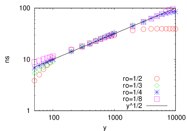
The approach-to-steady-state time scale $\tau_{ap}$ increases with $y$. $\tau_{ap}$ can exceed the mean axon lifetime $T$ by orders of magnitude (Fig. 3 and 4). Note that $\tau_{ap}$ is longer in a system with larger density of axons $\rho$ (Fig. 4). Ref.[11] discussed this point in detail. Further, asymptotically in $y$, we find $n_{\infty}=c+2\rho y^{b}\exp(-\beta y)$, with $b\approx 1/2$ (Fig. 5) – in good agreement with the mean-field prediction (Sec. IV).

Impact of interaction range: To test the impact of the range of inter-axon interaction, we have simulated a similar system with purely “contact” interaction, i.e., the interaction range is taken to be zero. With this reduction in the range of interaction, we find that the emerging time scales decrease. For instance, for a system of $L=800$ and $N_{0}=100$ the approach-to-steady-state time becomes $\tau_{ap}\lesssim 10T$. Thus an increase in the range of interaction increases the emerging time scales. The steady state distribution of fascicle sizes shows the same scaling behavior as in the case of nearest-neighbor interaction discussed in the following.

The steady state is characterized by the stationary distribution of fascicle sizes $P_{s}(n,y)$, defined as the number of fascicles of size $n$ at level $y$.

In this subsection, we review our analytical results from Ref. [11]. The following subsection presents new results for the time scales arising from the interaction of two neighboring fascicles.

The concept of effective single-fascicle dynamics has been introduced in Ref.[11]. The dynamics of a mean fascicle at level $y$ with $n(t)$ axons can be viewed as a stochastic process with gain rates $u_{+}(n)$ (for transitions $n\to n+1$) and loss rates $u_{-}(n)$ (for transitions $n\to n-1$). A fascicle loses axons only by the death of individuals, therefore, $u_{-}(n)=\beta n$ [11].

In absence of detachment events, any axon introduced within the basin (size $D$) of a fascicle (see Fig. 2(c)) can not escape the fascicle. Moreover, some of the axons born in the neighboring inter-basin gaps (size $E$) eventually join the fascicle under consideration. These two processes contribute to $u_{+}(n)$. As was shown in Ref. [11], the time series of $D(t)$ and $n(t)$ tend to co-vary. Thus treating the dynamics of $D$ as slave to $n$, we get a form $u_{+}=a+bn$ [11]. Note that the basin size $D$ can not exceed $2y$ or $L$, and $D>2y^{1/2}$ occurs with low probability. Therefore a saturation of $u_{+}(n)$ is expected for large values of $n$. The measured average gain and loss rates $u_{\pm}(n)$ obtained from our current simulations agree with the functional forms $u_{+}(n)=a_{+}+b_{+}n-c_{+}n^{2}$ and $u_{-}(n)=\beta n$ (data not shown). The quadratic correction to linear growth captures the saturation of $u_{+}(n)$ at large $n$.

The master equation of the growth-decay process for the effective single fascicle of size $n$ at level $y$ may be written as

for $n>1$. For the boundary state ($n=1$)

where $J_{+}(y)$ represents the rate with which new single axons appear between existing fascicles at $y$.

The solution of the master equation at steady state was derived in Ref. [11] and has the form,

where $\gamma=a_{+}/\beta-1$ and $\ell=1-b_{+}/\beta$ and $\kappa=c_{+}/2\beta$.

From the master equation one can estimate the approach-to-steady-state time $\tau_{ap}$ and the correlation time at steady state $\tau_{c}$ [11]. The correlation time $\tau_{c}$ for the fascicle size $n$, near the macroscopic stationary point $n_{s}$ [$u_{+}(n_{s})=u_{-}(n_{s})$] can be expressed [47] as $\tau_{c}=1/(u^{\prime}_{-}(n_{s})-u^{\prime}_{+}(n_{s}))=1/(\beta-b_{+}+2c_{+}n_{s})$. Under the linear approximation of $u_{+}(n)=a_{+}+b_{+}n$ the approach-to-steady-state time scale for the average fascicle size $\langle n\rangle$ can be written as $\tau_{ap}=1/(\beta-b_{+})$ [47].

Further, the mean lifetime of fascicles can be defined as $\tau_{f}=[\int_{1}^{\infty}P_{s}(n,y)dn]/J_{+}(y)$ and is evaluated to obtain [11]

Notice that the above derivations of the time scales already involved the numerical observation $u_{+}(n)=a_{+}+b_{+}n-c_{+}n^{2}$. Using the $y$-dependence of $b_{+}$ and $c_{+}$ obtained from numerical simulations, we found power law growth of the time scales, $\tau_{c}\sim y^{b}$, $\tau_{ap}\sim y^{b}$ and $\tau_{f}\sim y^{2b}$ with $b\approx 1/2$ [11].

In the following subsection, using a purely analytical, deterministic treatment of the dynamics of two neighboring fascicles, we show that a time scale growing as $y^{2b}$ emerges due to an exchange of basin size between the fascicles.

In this section we analytically explore the effective dynamics of two neighboring fascicles. Under the “always attach, never detach” rule the basins of neighboring fascicles do not overlap. Three dynamical variables characterize the dynamics of the fascicles: (i) the number of axons $n_{i}$ present in the fascicle, (ii) the basin size $D_{i}$ and (iii) the separation $E_{i}$ between the $i$-th and $(i+1)$-th basin (Fig. 2$(c)$). We explore the dynamics at a fixed $y$. We consider the thermodynamic limit of large $N_{0}$ and $L$ (with a fixed density $\rho=N_{0}/L$), and express all the length scales in units of $L$ and number of axons in units of $N_{0}$. Thus the reduced variables are $\eta_{i}=n_{i}/N_{0},~\lambda_{i}=D_{i}/L$, $\epsilon_{i}=E_{i}/L$, and the reciprocal system size $\tilde{a}=1/L$ has the meaning of a lower cut-off size in the continuum description. The effective equations of motion are

where $\delta=1/N_{0}$. First we describe the gain and loss terms in the dynamics of $\eta_{i}$. Axons born inside the basin of a fascicle contribute to the increase in $\eta_{i}$, hence the term $\beta\lambda_{i}$ (we used $N_{0}=\alpha/\beta$ to express axon birth rate $\alpha$ in terms of $\beta$). A fascicle can lose axons only by individual axon deaths, thus the loss term $\beta\eta_{i}$. Any axon which is born in the inter-fascicle empty spaces $\epsilon_{i-1}$ and $\epsilon_{i}$ ends up in either of the two neighboring fascicles with probability $1/2$, hence the gain term $(1/2)\beta(\epsilon_{i-1}+\epsilon_{i})$ ¹¹ 1 Notice that the fact that an axon born in a gap may end up as a single axon has been ignored as the corresponding rate becomes negligible at high $y$..

Next we consider the dynamics of basin size $\lambda_{i}$. A new axon can be born in the gap $\epsilon_{i}$ with a rate $\alpha(\epsilon_{i}-\tilde{a})$ and attach to the $i$-th fascicle with probability $1/2$. If it attaches it contributes half the gap size $\epsilon_{i}/2$ towards the basin size $\lambda_{i}$. Hence the gain term $(\alpha/4)\epsilon_{i}(\epsilon_{i}-\tilde{a})$. A similar contribution to the gain in the basin size comes from the other neighboring gap $\epsilon_{i-1}$. The death of a boundary axon reduces the basin size by an amount $\delta\lambda_{i}/(\eta_{i}-\delta)$ (assuming no double occupancy at a lattice point in the $y=0$ level). The contributions of this loss coming from two boundaries add up in the total loss term $2\times\beta\delta\lambda_{i}/(\eta_{i}-\delta)$.

Finally, we consider the dynamics of the inter-basin gaps $\epsilon_{i}$. The death of boundary axons of neighboring fascicles $i$ and $i+1$ that border the $i$-th gap $\epsilon_{i}$ contributes to the gain in the gap size. Thus the gain terms $\beta\delta\lambda_{i}/(\eta_{i}-\delta)$ and $\beta\delta\lambda_{i+1}/(\eta_{i+1}-\delta)$. Birth of an axon in the gap reduces the gap size under consideration. The rate of such an axon birth is $\alpha(\epsilon_{i}-\tilde{a})$ and on average this event reduces the gap size by an amount $\epsilon_{i}/2$. Thus the loss term $(\alpha/2)\epsilon_{i}(\epsilon_{i}-\tilde{a})$.

We use a periodic boundary condition, such that the last fascicle is a nearest neighbor of the first fascicle. These equations obey the constraint of overall constant size $\sum_{i}(\lambda_{i}+\epsilon_{i})=1$. It is important to note that the cut-off $\tilde{a}$ can be taken to zero meaningfully only after solving the differential equations.

For the simplest non-trivial case involving two fascicles, the steady state that follows from these equations is characterized by $\eta_{1}=\eta_{2}=1/2$, $\lambda_{1}=\lambda_{2}=1/2-\tilde{a}/2-2\delta-\tilde{a}\rho/16$ and $\epsilon_{1}=\epsilon_{2}=\tilde{a}/2+2\delta+\tilde{a}\rho/16$. We perform a normal mode analysis for small deviations from this steady state. The constraint $\sum_{i=1,2}(\lambda_{i}+\epsilon_{i})=1$ implies that there are only five independent deviations, $\delta\lambda_{1}$, $\delta\epsilon_{1}$, $\delta\epsilon_{2}$, $\delta\eta_{1}$ and $\delta\eta_{2}$. The linear stability analysis about the steady state shows that all the five possible modes are stable. Among them, four modes are short-lived. For them the deviations decay extremely fast with rates $\sim\beta$. However, the fifth mode which in the large-size limit can be written as

takes a long time to decay (see Fig. 8). It involves the loss of a boundary axon of one fascicle, which shrinks its basin size by $\delta D_{1}\approx-1/\rho$, and simultaneously a gain of a boundary axon for the other fascicle, increasing its basin size by the equal and opposite amount $\delta D_{2}\approx 1/\rho$. This operation leaves the inter-basin gap unchanged ($\delta E_{1}=0$) and can be viewed as an exchange of basin space (Fig. 8). The deviations from steady state in this mode decay over a very long time scale $\tau\approx{\bar{n}}^{2}/3\beta$ where $\bar{n}$ is the steady state value of the fascicle size ($n_{1}=n_{2}\equiv\bar{n}$).

Using the approximate growth of mean fascicle size $\bar{n}\sim y^{b}$ with $b=1/2$, we find a power law growth of this time scale $\tau\sim y^{2b}$. Notice that the measured time scales $\tau_{ap}$ and $\tau_{c}$ obtained from MC simulations show an increase with $y$ which approximately obeys the power law $y^{2b}$ with $b=1/2$ (see Fig.4). At lower densities, the simulated data agrees better with the $y^{2b}$ power law. In the analytic calculation above, we assumed single occupancy of the boundary sites of a fascicle basin (removal of a boundary axon was assumed to reduce the basin size). At higher densities this assumption dose not hold, the boundary of a basin does get multiply occupied by axons and thus we see a departure from the $y^{2b}$ power law.

The approach-to-steady-state time scale $\tau_{ap}$ decays with increasing detachment rates (decreasing inter-axon attraction $|E_{h}|$). We perform the approach to steady state data analysis in the same manner as we did for the purely energy-minimizing dynamics discussed in the previous section. This analysis gives an estimate of the time-asymptotic mean fascicle size $n_{\infty}$ as well as the approach-to-steady-state time scale $\tau_{ap}$ as a function of $y$. We perform this analysis for a system of $N_{0}=100$ and $L=200$ at various strengths of inter-axon interaction $E_{h}$. Strictly speaking, the presence of detachment invalidates our earlier mean field argument for the growth of fascicle size with $y$. While the concept of the basin of a fascicle is still meaningful, the basin can “leak”, i.e., newly growing axons can escape from it through the detachment process. Despite this, for most interaction strengths our numerical results obey $n_{\infty}=c+2\rho_{\rm{eff}}y^{1/2}\exp(-\beta y)$ with the fitting parameter $\rho_{\rm{eff}}$ taking the place of $\rho$ [Fig. 9($a$)]. The value of $\rho_{\rm{eff}}$ is the smallest for the weakest attractive interaction plotted in Fig. 9$(a)$. For extremely weak attraction (e.g., $E_{h}=-0.1$) almost no fasciculation can occur ($\rho_{\rm{eff}}\simeq 0$) and therefore $n_{\infty}$ remains independent of $y$ (data not shown).

As shown in Fig. 9($b$), the time scale $\tau_{ap}$ for the approach to steady state decays with reduced inter-axon attraction (i.e., with increased detachment rate). When $E_{h}\leq-2$, the growth of $\tau_{ap}$ with $y$ is similar to the one we observed for the “zero-temperature” dynamics. At $E_{h}=-1$, however, we find that $\tau_{ap}$ becomes comparable to the mean axonal lifetime $T$, even though at this value of $E_{h}$ the power-law growth of the mean fascicle size with $y$ is still maintained.

The reduction of $\tau_{ap}$ with increased detachment rate may be understood as a result of enhanced interaction between neighboring fascicles. As we noted before, the slowest time scale for the case of purely energy-minimizing dynamics is due to the very slow process of exchange of basin size between neighboring fascicles. In presence of finite detachment rates, axons from one fascicle can detach and connect to a neighboring fascicle, thereby opening up a new and faster mode of interaction between neighboring fascicles.

In this subsection we show that even in presence of an appreciable detachment rate ($E_{h}\leq-1$), the scaling of fascicle size distribution persists and the scaling function retains its overall functional form. However, with increasing detachment rates (decreasing $|E_{h}|$), the small $n$ portion of the fascicle size distribution gains at the cost of bigger fascicles and deviates from the scaling form.

Fig. 10 shows the steady-state fascicle size distributions for a system of $L=800$ and $N_{0}=100$. As the attraction is decreased from $E_{h}=-4$ to $E_{h}=-1$, we observe an overall increase in the small $n$ portion of the distribution. Except for the lowest values of $n$, we obtain data collapse implying the scaling form

where $r=2.1$ for $E_{h}=-4,\,-2$, and $r=2$ for $E_{h}=-1$. Similarly to the case of strictly energy-minimizing dynamics, this scaling is observed only in the intermediate range of $y$ values, $10^{3}<y<10^{4}$, and the scaling function is of the form $\phi(u)={\cal N}u\exp(-\nu u-\lambda u^{2})$ with $u=n/\langle n\rangle$.

The small-$n$ part of the distribution does not scale. $P_{s}(n,y)$ is large at $n=1$, and drops to lower values with increasing $n$, before it increases again to follow the scaling function. The functional form of the initial decay of $P_{s}(n,y)$ with $n$ depends on $y$ and also $E_{h}$, as we show in detail in Fig. 10$(d)$.

The discussion in this section shows that there are parameter regimes, e.g., the $E_{h}=-1$ case discussed above, where the emergent time scales are comparable to the mean lifetime $T$ of single axons, and at the same time the steady state statistics (the mean fascicle size and the fascicle size distribution) obey the overall features demonstrated by the energy-minimizing dynamics. This parameter regime might be utilized to attain a fasciculation pattern of this type in a relatively short time.

In this subsection we discuss the relation of our basic model, in which axons cannot detach from fascicles, to irreversible aggregation and coalescence processes.

Interpreting the fasciculation of axons with increasing $y$ (in a steady state configuration) as 1d irreversible aggregation of particles ($mA+nA\to(m+n)A$) [17, 46], we find a prediction $u\exp(-\lambda u^{2})$ (see equation 8.4.24 in  [17]) for the fascicle-size distribution, which is similar to the true distribution $u\exp(-\nu u-\lambda u^{2})$ (Sec. V.2) [11]. Note that the distribution obtained from the mapping to irreversible aggregation lacks the exponential part $\exp(-\nu u)$. As we explained in Ref. [11], having $\nu=0$ in our model would require $\tau_{\rm ap}=\infty$. The absence of the exponential part is therefore consistent with the absence of turnover-based dynamics in the 1d analogy.

The merging of fascicles with growing $y$ may alternatively be interpreted as an irreversible coalescence process $A+A\to A$ [16], viewing each fascicle as a particle $A$. The pattern formation in 1d irreversible coalescence had been quantified by the inter-particle distribution function (IPDF) [16], the distribution of distance between neighboring particles. The steady state of this process is trivial, a completely empty space. The IPDF is obtained at finite time $t$ before this steady state arrives, and has the form $(x/4{\cal D}t)\exp(-x^{2}/8{\cal D}t)$ where $\cal D$ denotes the particle diffusion constant [16]. The change in the inter-fascicle separation distribution with increasing $y$ in our model may be viewed as equivalent to the time evolution of IPDF in irreversible coalescence. This leads us to a prediction of the distribution of inter-fascicle separation $H(\Delta x,y)\approx(\Delta x/y)\,\exp(-\mu\,\Delta x^{2}/y)$. Using the same stochastic simulation that we used to obtain Fig. 6, we calculated the histogram of spatial separations $\Delta x$ between fascicles identified at various $y$-levels. Note that the separation between two neighboring fascicles $\Delta x$ is measured at the same $y$-level at which the fascicles are identified, and is different from the gap between fascicle basins $E$ (shown in Fig. 2). A rescaling of $H(\Delta x)$ by a factor $A(y)$ and $\Delta x$ by $B(y)$ leads to a data collapse (Fig. 11(a)), and approximate power law dependences $A\sim y^{p}$ and $B\sim y^{-q}$ with $p=0.96$ and $q=0.47$ (Fig. 11(b)). This result is in reasonable agreement with the above-mentioned form of $H(\Delta x,y)$ that predicts a scaling function ${\cal P}\Delta x\exp(-{\cal Q}\Delta x^{2})$ (Fig. 11(a)), and scaling exponents $p=1$ and $q=1/2$.

In this subsection we discuss analogies of our model of axon fasciculation in presence of detachment to reversible aggregation and coalescence processes in 1d. Due to specific features of our model, only qualitative analogies to models from the 1d literature can be made.

Detachment events are partially captured when the axon fasciculation with increasing $y$ in a fixed-time configuration is formally viewed as a 1d diffusion with reversible aggregation, the chipping model: $mA+nA\rightarrow(m+n)A$ and $mA\rightarrow(m-1)A+A$ [18], denoting each axon by a particle $A$. (Note, however, that steady state configurations of our model show splitting of fascicles with increasing $y$ (e.g., see Fig. 2(b)) into two fascicles containing multiple axons. The chipping model does not include the analog of such a process). The chipping model posseses a non-trivial steady state ($t\rightarrow\infty$, corresponding to $y\rightarrow\infty$ within our model). It shows a dynamic phase transition associated with particle density $\rho$ [18, 19]. The steady state distribution of clusters of size $n$ is predicted to be $P_{s}(n)\sim\exp(-n/n^{\ast})$ at $\rho<\rho_{c}=\sqrt{1+w}-1$, where $w$ denotes a constant single particle chipping rate. At the critical density $\rho=\rho_{c}$, the distribution changes its shape to $P_{s}(n)\sim n^{-5/2}$. At density above $\rho_{c}$ this power-law distribution remains unaltered, and in addition to the power law distributed clusters one gets a single cluster of diverging size [18]. Fig. 10 shows fascicle size distributions obtained from our model at various interaction strengths $E_{h}$. Note that, in contrast to the chipping model, in our model the rate $w=1/[1+\exp(-nE_{h})]$, with which a single axon detaches from a fascicle, depends on the fascicle size $n$. Only for the weakest interaction $E_{h}=-0.1$ (inset of Fig. 10(d)), the detachment rate from a two-axon fascicle $w=0.45$ corresponds to a critical density $\rho_{c}=0.2$ which is greater than the axon density $\rho=1/8$. The corresponding fascicle size distribution shows a form consistent with $\sim\exp(-n/n^{\ast})$ (inset of Fig. 10(d)). For $E_{h}=-1$ the detachment rate from a two-axon fascicle $w=0.12$ corresponds to a critical density $\rho_{c}=0.06<\rho$ ($=1/8$). The fascicle size distribution in the region of small $n$, for $E_{h}=-1$, shows rough agreement with the power law $\sim n^{-5/2}$ (Fig. 10(d)). This change in shape of the fascicle size distribution from an exponential decay to a power-law decay at small $n$, thus, is consistent with the dynamical phase transition predicted by the chipping model. Since in our model the detachment rate of axons exponentially decays with fascicle size $n$, for larger fascicles the detachment rate $w$ gets so small that the analogy with the reversible chipping model breaks down, and the behavior of the system becomes analogous to irreversible aggregation. The fascicle size distribution in the region of larger $n$ (Fig. 10) becomes indistinguishable from axon fasciculation in absence of detachment.

We note that, for our model in presence of detachment, the change in the distribution of inter-fascicle spatial separation with increasing $y$ can not be easily understood in terms of reversible coalescence $A+A\rightleftharpoons A$ [16, 48] (denoting each fascicle as a particle $A$). The main reasons are: (i) the reverse reaction $A\to A+A$ allows for splitting of a single axon into two, a mechanism not allowed in our model; (ii) in contrast to reversible coalescence, the probability of splitting of a fascicle in our model decays rapidly with increasing fascicle size. Thus the $y$-independent distribution of inter-fascicle separation $c_{s}\exp(-c_{s}\Delta x)$, expected from IPDF of reversible coalescence [16], is never reached. At large $y$, we find a distribution of inter-fascicle separation that conforms more to ${\cal P}\Delta x\,\exp(-{\cal Q}\,\Delta x^{2})$ (data not shown), consistent with irreversible coalescence (see previous subsection).

We note again that time-dependent quantities in our model have no analog in the mapping to the 1d models we discussed above. The emergence of density-dependent long time scales in reversible coalescence [16, 48, 49] therefore has no relation to the long time scales in our model, which are due to a very slow reorganization of fascicle basins (Sec. V.4) — a consequence of axon turnover.

Let us consider a system containing two types of axons named $r$ and $b$. Assume that a fascicle contains $n^{r}$ of $r$-axons and $n^{b}$ of $b$-axons. If the $i$-th axon in the fascicle is of type $r$, the purity of environment that this axon encounters within the fascicle is $s_{i}=(n^{r}-n^{b})/(n^{r}+n^{b})$, while if the axon is of type $b$, the purity of environment is $s_{i}=(n^{b}-n^{r})/(n^{r}+n^{b})$. Then the mean purity of environment obtained by averaging over all $N(y)$ axons is $S=(\sum_{i=1}^{N(y)}s_{i})/N(y)$. The partial sum within a fascicle gives $n^{r}(n^{r}-n^{b})/(n^{r}+n^{b})+n^{b}(n^{b}-n^{r})/(n^{r}+n^{b})=(n^{r}-n^{b})^{2}/(n^{r}+n^{b})$. Thus, the degree of sorting can be quantified as the mean purity of axon environment

Notice that $0\leq S\leq 1$; $S=1$ corresponds to completely pure fascicles containing only one type of axons, whereas $S=0$ describes fascicles containing an equal mixture of the two axon types.

We consider a system of size $L=800$ having $N^{r}_{0}=50$ axons of type $r$ and $N^{b}_{0}=50$ axons of type $b$ at the $y=0$ level ($\rho=(N^{r}_{0}+N^{b}_{0})/L=1/8$). We use the homotypic interaction energy (interaction between $r$-$r$ or $b$-$b$) $E_{h}=-4$ and the heterotypic interaction energy (between the two different types $r$-$b$) $E_{o}=-0.1$. We monitor the time evolution of the mean purity of environment $S$ and the mean fascicle size $\bar{n}$. A typical configuration is shown in Fig. 2$(b)$. The mean fascicle size reaches the steady state value at each $y$-level with two characteristic time scales, similarly to the case of a system containing only one type of axons (Fig. 3). The shorter time scale is intrinsic, the mean lifetime of a single axon $T$, and the other one is the emergent approach-to-steady-state time scale $\tau_{n}$ (equivalent to $\tau_{ap}$ defined in the caption of Fig. 3). As in the case of a system containing only one type of axons, this time scale $\tau_{n}$ can be orders of magnitude larger than $T$ (Fig. 12$(d)$).

The intrinsic time scale $T$ does not appear in the dynamics of $S$, however. $S$ approaches its steady state value $S_{\infty}$ with a single time scale $\tau_{s}$. The measured mean purity $S$ fits to the form $S=S_{\infty}+r\exp(-t/\tau_{s})$ (Fig. 12($a$)). The steady-state mean purity $S_{\infty}$ initially grows with $y$, reaching a maximum beyond which $S_{\infty}$ decreases (Fig. 12($b$)). This non-monotonic behavior is seen both for low ($\rho=1/8$) and high ($\rho=1/2$) density systems (Fig. 12($b$)). Thus for the combination of strong homotypic and weak heterotypic attractive interaction, the fascicles achieve the highest purity at a particular distance from their starting point, beyond which the typical fascicle keeps on losing purity. From energetic considerations, one may understand this behavior as follows. The high strength of the homotypic attraction compared to the heterotypic one leads to sorting and thus the initial growth in purity at lower $y$-levels. Once one obtains highly pure and sufficiently large fascicles, however, the heterotypic interaction will merge the $r$-dominated and $b$-dominated fascicles to form larger mixed fascicles, and thereby lead to a loss in mean purity. The effect of the weak heterotypic interaction becomes significant only at higher $y$-levels, where large fascicles are formed (recall that in our model, the interactions are additive).

Similar to the case of a system containing only a single axon type in presence of detachment, we find that the steady state mean fascicle size grows as $n_{\infty}=c+2\rho_{\rm{eff}}y^{1/2}\exp(-\beta y)$. Fig. 12($c$) shows that the subtracted mean fascicle size $n_{s}=(n_{\infty}-c)\exp(\beta y)/2\rho_{\rm{eff}}$ follows the power law $y^{b}$ with $b=1/2$. The effective density $\rho_{\rm{eff}}$ and offset fascicle size $c$ are treated as fitting parameters.

The time scales for approach to steady state $\tau_{n}$ and $\tau_{s}$ grow with $y$ following an approximate power law $y^{2b}$ with $b=1/2$ [Fig. 12($d$)]. This behavior is seen to be independent of density $\rho$, in contrast to the single-type case, where we found reliable $y^{2b}$ growth of the emergent time-scales only at lower densities. Recall that, reduced inter-axon interaction strengths lead to lower effective densities $\rho_{\rm{eff}}$ (Fig. 9$(a)$). In the present case of mixed population of axons of two types, the heterotypic interaction is very weak and may have lead to the effectively low-density ($y^{2b}$) power-law growth. We note that $\tau_{n}$ and $\tau_{s}$ turn out to be approximately equal to each other at all $y$-levels.

In this section we briefly discuss the distribution of fascicle composition $P(n^{r},n^{b})$, measured as the number of fascicles with $n^{r}$ $r$-axons and $n^{b}$ $b$-axons at a specified $y$-level and time $t$. In Fig. 13 we show this distribution obtained by collecting data within the time interval $10T\leq t\leq 15T$ at various $y$-levels for a system of $N^{r}_{0}=N^{b}_{0}=50$ and $L=200$ ($\rho=1/2$). From the approach-to-steady-state data (Fig. 12) it is clear that at $t=10T$, steady state is reached only up to $y\approx 100$. Thus the distributions obtained at $y=10^{3},\,10^{4}$ in Fig. 13 are far from steady state ³³ 3 To obtain sufficiently good statistics for $P(n^{r},n^{b})$, it was necessary to average over a large number of configurations. Consequently we were restricted to a lower range of $t$ as compared to the data for mean fascicle size $n$ and purity $S$ shown in Fig. 12.. All the plots in Fig. 13 show a pronounced maximum for evenly mixed fascicles, meaning that most of the fascicles we obtain are mixed by type. However, a careful look at the plots reveals off-peak features of the distribution with reasonable weight that reflect the presence of fascicles with highly asymmetrical composition (e.g., along the $n^{b}=1$ line for the plot at $y=100$ in Fig. 13, the maximum of the distribution is at $n^{r}=5$).