Rational Terms in Theories with Matter

Preprint: HRI/ST/1005

Shailesh Lal Affiliation: Harish-Chandra Research Institute Suvrat Raju Affiliation: Chatnag Marg, Jhunsi, Allahabad 211019.

Abstract:

We study rational remainders associated with gluon amplitudes in gauge theories coupled to matter in arbitrary representations. We find that these terms depend on only a small number of invariants of the matter-representation called indices. In particular, rational remainders can depend on the second and fourth order indices only. Using this, we find an infinite class of non-supersymmetric theories in which rational remainders vanish for gluon amplitudes. This class includes all the “next-to-simplest” quantum field theories of arXiv:0910.0930. This provides new examples of amplitudes in which rational remainders vanish even though naive power counting would suggest their presence.

Keywords:

S-matrix, non-Abelian gauge theories, rational terms, indices

1 Introduction

Scattering amplitudes in four dimensional gauge theories have been the subject of several recent studies [1]–[11]. Much of this work has focussed on amplitudes in ${{\mathcal{N}}=4}$ super-Yang-Mills (SYM) or in pure Yang-Mills and has involved the development of new techniques to study S-matrix elements in these theories. However, these techniques apply far more generally. Furthermore, they are capable of shedding fresh light even on familiar and well-studied systems. In this spirit, in a previous paper, we considered gluon scattering amplitudes in gauge theories coupled to matter in arbitrary representations [12].

Using Forde’s technique for extracting one-loop integral coefficients [13, 8] we showed that triangle and bubble coefficients in such theories were proportional only to a small number of invariants of the matter representation. These invariants are called indices.¹¹ 1 The second order index $I_{2}(R)={{\rm Tr}_{R}\left(T^{a}T^{b}\right)\over 2{\rm Tr}_{F}\left(T^{a}T^{b}\right)}$ is probably familiar to the reader. As we review later, the trace of a product of any number of generators can be expanded in terms of the invariant tensors of the algebra multiplied by coefficients called indices. The higher indices are closely related to the higher Casimir invariants. Using this information, we were able to find new examples of theories in which gluon scattering amplitudes were free of triangles and/or bubbles.

In this paper, we extend this argument to show that rational terms associated with gluon amplitudes in theories with matter are also proportional to the first few indices (up to the fourth order indices) of the matter representation.²² 2 We should clarify that boxes, triangles and bubbles come with associated rational terms. In this paper, we use the phrase “rational terms” to refer to the rational remainders that are not associated with these integral functions. This surprising result follows from the newly developed method of extracting rational terms by considering the large-mass limit of massive particles propagating in the loop [14].

Rational terms are notoriously difficult to extract since they are missed by four dimensional unitarity cuts. One has to resort either to $d$ -dimensional unitarity [15, 16, 17, 18, 19, 20] or to other techniques like on-shell recursion at one-loop [21, 22, 23]. However, for our purposes the most useful approach is the one developed by Badger [14]. Here, a massless d-dimensional particle propagating in the loop is traded for a massive 4-dimensional particle and rational terms are extracted by examining the behaviour of unitarity cuts at large mass.

This approach reveals the remarkably simple structure of rational terms in gluon amplitudes referred to above. The fact that the rational contribution of matter to gluon amplitudes can be written in terms of the first few indices of the matter representation implies that the condition that rational terms vanish can now be expressed in terms of linear Diophantine equations involving these indices. We solve these equations to find an infinite class of non-supersymmetric theories in which rational terms vanish for gluon amplitudes. This set includes, but is not limited to, the set of next-to-simplest quantum field theories of [12].

This is interesting because these theories are not naively cut-constructible. Supersymmetric theories are cut-constructible because the expansion of an amplitude in terms of Feynman diagrams can be organized to show that two powers of the momentum cancel between fermions and bosons [24, 25]. In our examples, naively counting the powers of momentum that appear in Feynman diagrams would lead one to suspect that rational terms should be present. In this sense the unexpected simplifications that are present in our theories are similar to those seen in ${{\mathcal{N}}=8}$ supergravity [26] and QED [27].

An overview of this paper is as follows. In section 2, we review the results of our previous paper. In section 3, we show that rational terms associated with gluon amplitudes are proportional to the second and fourth order indices of the matter representation. In section 4, we write down the condition for gluon amplitudes to be free of rational terms and find new examples of theories in which these are cut-constructible. We conclude in section 5. The appendix contains some group-theoretic details.

2 Review

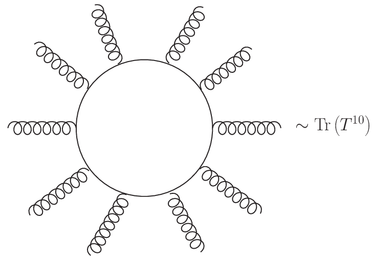
Let us briefly review how triangle and bubble coefficients for gluon amplitudes in gauge-theories coupled to matter turned out to be proportional to only a few indices of the matter representation. Naively, we would not expect this at all. For example, consider the following Feynman diagram (Fig. 1) for a 10-point gluon amplitude with a massless fermion in the loop.

This Feynman diagram is proportional to ${\rm Tr}(T^{a_{1}}T^{a_{2}}\ldots T^{a_{10}})$ where $a_{1},\ldots a_{10}$ are colors associated with the gluon lines. So, naively one would certainly not expect that one-loop integral coefficients for a scattering amplitude of an arbitrary number of gluons would be sensitive only to the trace of a small number of generators.

Refer to caption — Figure 1: A Matter-Loop

Of course, we also know that the one-loop $\beta$ function for the gauge-coupling simplifies and is proportional to the quadratic index only. It turns out the coefficients of triangles and bubbles also simplify similarly. They are not as simple as the one-loop $\beta$ function and depend on the higher-indices also. Triangles can depend on the sixth order indices (these are what appear when we expand the trace of six generators in terms of the invariant tensors of the algebra), while bubbles can depend on the fourth order indices. More precisely, the contribution of a scalar or a fermion in representation $R_{s/f}$ to a triangle coefficient — $B$ — and a bubble coefficient — $C$ — associated with a gluon amplitude can be written as (in the notation of [12])

\begin{split}B_{s/f}&=\sum_{n=2,4,5,6}\omega^{B}_{a_{1}\ldots a_{n}}{\rm Tr}_{R_{s}/R_{f}}(T^{(a_{1}}\ldots T^{a_{n})}),\\ C_{s/f}&=\sum_{n=2,4}\omega^{C}_{a_{1}\ldots a_{n}}{\rm Tr}_{R_{s}/R_{f}}(T^{(a_{1}}\ldots T^{a_{n})}),\quad\text{in non-supersymmetric~theories.}\end{split}

(1)

We emphasize that this result holds for an arbitrary number of external gluons.

For supersymmetric theories, these results simplify. For a chiral multiplet in representation $R_{\chi}$ , triangle coefficients can depend on the higher indices up to the fifth order indices while bubble coefficients only depend on the quadratic index i.e.

\begin{split}B_{\chi}&=\sum_{n=2,4,5}\omega^{B}_{a_{1}\ldots a_{n}}{\rm Tr}_{R_{\chi}}(T^{(a_{1}}\ldots T^{a_{n})}),\\ C_{\chi}&=\omega^{C}_{a_{1}a_{2}}I_{2}(R_{\chi})\kappa^{a_{1}a_{2}},\quad\text{in supersymmetric~theories,}\end{split}

(2)

where $\kappa$ is the Killing form.

This leads to an interesting possibility. Since triangles and bubbles are sensitive only to a small number of invariants of the representation and not to the full-character, we can replace the adjoint matter of the ${{\mathcal{N}}=4}$ SYM theory with matter in a different representation that has the same first few indices. In this way, one can mimic the adjoint representation as far as the triangle and bubble coefficients are concerned.

In fact, demanding that the theory be free of triangles and bubbles leads to linear Diophantine equations involving these higher-order indices. This is because any representation can be decomposed in terms of irreducible representations

R=\bigoplus n_{i}R_{i}.

(3)

Since the indices are linear, mimicking the first few indices of the adjoint leads to linear equations in the $n_{i}$ (which are, of course, constrained to be natural numbers). More precisely, the conditions for supersymmetric and non-supersymmetric theories to be free of triangles and/or bubbles can be written as in Table 1.

Condition (C): ${\rm Tr}_{\rm R}(\Pi_{i=1}^{n}T^{a_{i}})=m\,{\rm Tr}_{\rm adj}(\Pi_{i=1}^{n}T^{a_{i}}),~n\leq p$
Non-susy theories have	only boxes	no bubbles
if $R_{f}$ satisfies C with	p=6, m=4	p=4,m=4
and $R_{s}$ satisfies C with	p=6, m=6	p=4,m=6.
Susy theories have	only boxes	no bubbles
if $R_{\chi}$ satisfies C with	p=5, m=3	p=2,m=3.

Table 1: Conditions for the S-matrix to simplify

In our previous paper, we solved these equations. In the planar limit, there are several theories including the ${\mathcal{N}}=2,SU(N)$ theory with $2N$ fundamental hypermultiplets, in which gluon amplitudes are free of triangles and bubbles. We found two examples where these properties persisted even for the non-planar sector. One of these — the ${{\mathcal{N}}=2}$ SYM theory with a symmetric and an anti-symmetric tensor hypermultiplet — is an orientifold of the ${{\mathcal{N}}=4}$ theory but the fact that its amplitudes at all $N$ are as simple as those of the ${{\mathcal{N}}=4}$ theory goes beyond planar equivalence.

We also found several example of non-supersymmetric theories that were free of bubbles but had triangles. These theories will make another appearance below where we show that they are all also free of rational terms.

3 Rational Terms in Theories with Matter

We now turn to a study of rational terms associated with gluon amplitudes in theories coupled to matter in arbitrary representations. As we review below, gluon amplitudes in supersymmetric theories are cut-constructible [24]. This means that the contribution of fermions, in any representation, to rational terms is the same (up to a minus sign) as that of scalars. Hence, it is sufficient to consider the contribution of scalars to rational terms. This is what we do below.

As we mentioned above, our tool will be the method of extracting rational terms by trading a d-dimensional massless scalars for a 4 dimensional massive scalar. Rational terms come from the large-mass limit of massive unitarity cuts. We will find that the behaviour of tree-amplitudes simplifies in this limit. This means that integral coefficients and the rational terms that they imply also simplify.

3.1 Review

We now quickly review the argument that rational terms vanish in supersymmetric theories [24, 25]. We focus on gluon amplitudes. One-loop gluon amplitudes can be obtained from the 1PI effective action. The 1PI effective action for the gauge field, in the presence of scalars and fermions can be calculated in background field gauge and written as

\begin{split}i\Gamma[A]&={-i\over 4g^{2}}(F_{\mu\nu}^{a})^{2}+i{\mathcal{L}}_{\text{c.t.}}-{1\over 2}\ln\text{det}_{[1]}\Delta_{\text{adj},1}+\ln\text{det}_{[0]}\Delta_{\text{adj},0}\\ &+{n_{f}\over 2}\ln\text{det}_{[1/2]}\Delta_{R_{f},{1\over 2}}-{n_{s}\over 2}\ln\text{det}_{[0]}\Delta_{R_{s},0},\end{split}

(4)

where the first two determinants come from the gauge field and ghosts and the next two come from the fermions and scalars respectively. (See [28] for a derivation of this result.) For us, it is only important that the generalized d’Alembertians $\Delta_{r,j}$ have the form

\Delta_{r,j}=-\partial^{2}+i\left[\partial^{\mu}A_{\mu}^{a}T^{a}_{r}+A_{\mu}^{a}T^{a}_{r}\partial^{\mu}\right]+A^{a\mu}T^{a}_{r}A_{\mu}^{b}T^{b}_{r}+F^{b}_{\rho\sigma}J_{j}^{\rho\sigma}T^{b}_{r}.

(5)

where $J_{j}$ is the generator of Lorentz transformations for spin $j$ and the $T^{a}$ are the generators of gauge transformations for representation $r$ .

Now, all one-loop amplitudes can be obtained by attaching tree-graphs to the one-loop vertices obtained by expanding these determinants. Consider the one-loop integrals that result from expanding (4) in powers of $A$ . Those integrals that have the same number of momenta in the numerator as propagators in the denominator can have no insertion of the last term in (5) involving $F\cdot J$ ; hence, they cancel in supersymmetric theories. Furthermore, since ${\rm Tr}(J_{1})={\rm Tr}(J_{1\over 2})=0$ , we must have at least two insertions of $F\cdot J$ . A loop-integral with two insertions of this term must have at least two powers of momentum less in the numerator than in the denominator. This is enough to ensure that rational terms vanish in supersymmetric theories.

Hence, the contribution of scalars, in a certain representation, to rational terms is the same as the contribution of fermions in the same representation. So, we can obtain all the information we want just by considering scalars.

Note, that the formula (4) itself does not tell us much about the contribution of scalars to rational terms. In fact, naively expanding the determinants using (5) would lead us to believe that we obtain traces of an arbitrary number of generators. As we see below, this is not correct.

The contribution of scalars to rational-terms can be conveniently obtained using the methods of [14]. We take the scalar propagating in the loop to be massive, with mass $\mu$ , and then pick out specific coefficients of $\mu$ in the box, triangle and bubble coefficients.

3.2 Boxes

The box coefficient is calculated through a product of four tree-amplitudes. When we consider the contribution of scalars to the box coefficient, each of these tree-amplitudes has two scalars apart from an arbitrary number of external gluons. According to [14], we need to assign mass $\mu$ to these intermediate scalars and then extract the coefficient of $\mu^{4}$ in the box-coefficient.

So, consider the coefficient for the box with momenta $q_{1}\ldots q_{4}$ at the vertices. This coefficient is calculated by making a 4-cut. The cut-momenta are calculated explicitly in [14]. For us, it is only important that for large internal mass $\mu$ , the momentum behaves like:

p=p_{0}(\mu)+\left|\mu\right|\chi,

(6)

where $\chi^{2}=1$ and $\underset{\mu\rightarrow\infty}{\lim}{p_{0}\over\mu}=\underset{\mu\rightarrow\infty}{\lim}{p_{0}\cdot\chi}=0$ .

We are concerned with the product of 4 tree-amplitudes, each with two scalars and an arbitrary number of gluons. The first of these has scalar momenta $p,p+q_{1}$ . To analyze this tree-amplitude we go to a gauge where the gauge field satisfies

\chi\cdot A(q)=0.

(7)

Now, every propagator comes with a factor of ${1\over\mu}$ as for example in the figures in the second and third line (Figs. 3 – 6) of Table 2.

[Uncaptioned image] — Table 2: Dominant diagrams at large $z$

1.	2.
3.	4.
5.	6.

The only time we get a factor of $\mu$ in the numerator is when $q=q_{1}$ . This is because $\chi\cdot q_{1}=0$ and so the gauge choice (7) is not possible. This interaction is shown in the first line (Fig. 1) of Table 2. This tells us that the tree-amplitude has the form

{\mathcal{A}}(p,p+q_{1})=|\mu|c_{a}T^{a}+{c_{ab}\over 2}\{T^{a},T^{b}\}+\ldots

(8)

where $T^{a}$ are the generators of the scalar-representation $R$ .

In fact we can repeat the analysis of [12] to show that, for large $\mu$ , the $n$ -pt tree-amplitude goes like

{\mathcal{A}}(p,p+q_{1})=\sum_{k=1}^{n}{c_{a_{1}\ldots a_{k}}T^{(a_{1}}\ldots T^{a_{k})}\over|\mu|^{k-2}},

(9)

where $c\underset{\mu\rightarrow\infty}{\longrightarrow}{\rm O}\left({1}\right)$ .

In particular, if we want the $\mu^{4}$ term in the product of four tree-amplitues, we have to take the leading term in the expansion (9) for each tree-amplitude. Moreover, we need to sum over all scalar colors to get the box coefficient; this leads to a trace. So, we find that

\sum{\mathcal{A}}_{1}{\mathcal{A}}_{2}{\mathcal{A}}_{3}{\mathcal{A}}_{4}=\mu^{4}c^{1}_{a_{1}}c^{2}_{a_{2}}c^{3}_{a_{3}}c^{4}_{a_{4}}{\rm Tr}_{R}\left(T^{a_{1}}T^{a_{2}}T^{a_{3}}T^{a_{4}}\right)+{\rm O}\left({|\mu|^{3}}\right).

(10)

The box coefficient is given by further summing this over the two choices of cut momenta. This implies that the rational contributions from the box-terms can depend on, at most, the fourth indices of the matter representation. More precisely, the rational contribution from the box-coefficient, $R_{A}$ can be written as

R_{A}=\omega^{A}_{i_{1}i_{2}}{\rm Tr}_{R}\left(T^{i_{1}}T^{i_{2}}\right)+\omega^{A}_{i_{1}i_{2}i_{3}i_{4}}{\rm Tr}_{R}\left(T^{(i_{1}}T^{i_{2}}T^{i_{3}}T^{i_{4})}\right).

(11)

Here, we follow the conventions of [12] so that a complex scalar in representation $r$ has $R=r+\overline{r}$ . The advantage of this notation is that it makes manifest the fact that symmetrized traces of an odd number of generators never appear in the scalar contribution. (Another way to see this cancellation is to recall that we need to sum over the two possible orientations of the scalar line in the loop.)

3.3 Triangles

Rational terms also come from the ${\rm O}\left({\mu^{2}}\right)$ term in triangle-coefficients. To extract triangle coefficients, we make a 3-cut. The 3-cut leaves us with one free parameter $z$ . There are several equivalent ways of fixing this parameter and extracting the triangle coefficient [13, 8, 29]. We stick to the conventions of [13]. As the reader can verify using the detailed formulas in [14] (we use $z$ instead of $t$ ), the cut-momentum behaves like

p=\chi_{0}+z\chi_{1}+{\mu^{2}\over z}\chi_{2}.

(12)

What is important for us is that

\chi_{1}^{2}=\chi_{2}^{2}=0;\quad\chi_{1}\cdot\chi_{2}=1;\quad\chi_{1}\cdot\chi_{0}={\rm O}\left({1\over z}\right);\quad\chi_{2}\cdot\chi_{0}=0.

(13)

The three-cut momenta are $p,p+q_{1},p-q_{3}$ . We now wish to take the product of three-amplitudes with two scalars each and several gluons. The rational term depends on the coefficient of $z^{0}\mu^{2}$ in this product

R_{B}={1\over 2}\sum\left.{\mathcal{A}}_{1}{\mathcal{A}}_{2}{\mathcal{A}}_{3}\right|_{z^{0}\mu^{2}},

(14)

where the sum is over the intermediate scalar colors and the two solutions for the loop momentum and the coefficient is extracted by series expanding first with respect to $z$ around $z=\infty$ and then with respect to $\mu$ around $\mu=\infty$ .

An amplitude with scalar momenta $p,p+q_{1}$ is dominated by a few diagrams in the gauge

\chi_{1}\cdot A(q)=0.

(15)

The leading-diagram involves a single scalar-gluon interaction as in Fig. 1 of Table 2. Other than this, we also need to consider Figs. 2 and 3 of that table. Finally, there are the two diagrams shown in Figs. 4 and 5. Note that each of these would seem to give a contribution to the symmetrized product of 3-generators that goes like ${\mu^{2}\over z^{2}}$ . This combines a ${\mu^{2}\over z}$ from the 3-pt vertex with a ${1\over z}$ from the propagator. However, notice that this term exactly cancels between the two diagrams. The diagram in Fig. 6 contributes to a 3-generator term (the symmetrized 4-generator term cancels with a ‘flipped’ diagram) without a $\mu^{2}$ . Adding all these contributions, we find that the behaviour at large $z$ and large $\mu$ of a tree-amplitude is

A=(a_{i}z+b_{i}{\mu^{2}\over z})T^{i}+(a_{i_{1}i_{2}}+b_{i_{1}i_{2}}{\mu^{2}\over z^{2}})T^{(i_{1}}T^{i_{2})}+({a_{i_{1}i_{2}i_{3}}\over z}+{b_{i_{1}i_{2}i_{3}}\mu^{2}\over z^{3}})T^{(i_{2}}T^{i_{2}}T^{i_{3})}+{\rm O}\left({1\over\mu}\right).

(16)

From here it directly follows that the rational contribution from triangles which comes from the $z^{0}\mu^{2}$ term in the product of three-amplitudes must go like

R_{B}=\omega^{B}_{i_{1}i_{2}}{\rm Tr}_{R}\left(T^{i_{1}}T^{i_{2}}\right)+\omega^{B}_{i_{1}i_{2}i_{3}i_{4}}{\rm Tr}_{R}\left(T^{(i_{1}}T^{i_{2}}T^{i_{3}}T^{i_{4})}\right),

(17)

and so, can depend, at most on the fourth index.

3.4 Bubbles

The contribution of bubble coefficients to the rational remainder is again obtained by extracting the ${\rm O}\left({\mu^{2}}\right)$ piece of the bubble coefficient at large $\mu$ . The bubble coefficient is extracted from the two-cut which now leaves two parameters free. An analysis very similar to the analysis above shows that the rational contribution from bubbles can only depend on the quadratic Index.

R_{C}=\omega^{C}_{i_{1}i_{2}}{\rm Tr}_{R}\left(T^{i_{1}}T^{i_{2}}\right)=\omega^{C}_{i_{1}i_{2}}I_{2}(R)\kappa^{i_{1}i_{2}}.

(18)

This may be seen by parameterizing the two-cut in the form given in [14, 13] but perhaps the easiest way to see this result is to use the method of [29]. Here, the two-cut is parameterized by putting additional restrictions on a momentum of the form (12). There are two contributions to the bubble-coefficient; one depends on the $\mu^{2}z^{2}$ term in the product of three-amplitudes and another depends on the $\mu^{2}z^{i},i=0\ldots 2$ term in the product of two tree-amplitudes. Given the behaviour of the tree-amplitude (16), we can see that these terms can depend on, at most, the quadratic index.

4 Cut-Constructible Theories

From here, we see that it is quite easy to find new cut constructible theories. This is because, we just need to satisfy the equation

{\rm Tr}_{R_{f}}\left(T^{(a_{1}}\ldots T^{a_{n})}\right)-{1\over 2}{\rm Tr}_{R_{s}}\left(T^{(a_{1}}\ldots T^{a_{n})}\right)={\rm Tr}_{\rm adj}\left(T^{(a_{1}}\ldots T^{a_{n})}\right),n=2,4.

(19)

Recall that in (19), we follow the conventions of [12], which are explained below (11), and count in terms of real scalars and Weyl-fermions. Note that for $n=3$ , the fermionic trace must vanish for anomaly cancellation.

The reader might worry that (19) leads to a very large number of independent equations. For example, for $SU(N)$ , one might be led to believe that (19) consists of ${\rm O}\left({N^{8}}\right)$ independent equations corresponding to distinct choices of generators.

In fact, (19) is very simple and leads to just three independent equations.³³ 3 For the group $SO(8)$ , there are four independent equations. This is because there are two independent invariant tensors of rank $4$ . Equation (20) must also be suitably modified. This is because the symmetrized trace of two and four generators can be expanded as

\begin{split}&{1\over 2}{\rm Tr}_{R}\{T^{a_{1}},T^{a_{2}}\}=I_{2}(R)\kappa^{a_{1}a_{2}},\\ &{\rm Tr}_{R}\left[T^{(a_{1}}T^{a_{2}}T^{a_{3}}T^{a_{4})}\right]=I_{4}(R)d^{a_{1}a_{2}a_{3}a_{4}}+I_{2,2}\kappa^{(a_{1},a_{2}}\kappa^{a_{3}a_{4})}.\end{split}

(20)

The symmetrized trace of 3-generators never appears. For complex scalars and Dirac fermions this trace cancels when the different contributions to a cut are summed over. For real or pseudoreal representations this trace is zero while for Weyl fermions in complex representations, this trace must vanish by anomaly cancellation.

Now, expanding the scalar and fermionic representations in terms of irreducible representations as

R_{f}=\oplus n_{i}^{f}R_{i}^{f},\quad R_{f}=\oplus n_{i}^{s}R_{i}^{s},

(21)

we find (19) can be written as the three-equations

\begin{split}\sum_{i}\left(n_{i}^{f}I_{2}(R_{i}^{f})-{n_{i}^{s}\over 2}I_{2}(R_{i}^{s})\right)&=I_{2}({\rm adj}).\\ \sum_{i}\left(n_{i}^{f}I_{2,2}(R_{i}^{f})-{n_{i}^{s}\over 2}I_{2,2}(R_{i}^{s})\right)&=I_{2,2}({\rm adj}).\\ \sum_{i}\left(n_{i}^{f}I_{4}(R_{i}^{f})-{n_{i}^{s}\over 2}I_{4}(R_{i}^{s})\right)&=I_{4}({\rm adj}).\end{split}

(22)

For the exceptional groups and also for $SU(2),SU(3)$ , there are only two independent equations since $I_{4}$ vanishes. For $SO(8)$ , there is an additional equation since there are two independent fourth-order indices.

The equations (22) are a set of linear Diophantine equations in the variables $n_{i}$ . In fact, given any solution to the equation

\sum_{i}n_{i}I_{\alpha}(R_{i})=0,\quad n_{i}\in{\mathcal{Z}},

(23)

where $I_{\alpha}$ runs over the set $I_{2},I_{2,2},I_{4}$ , subject to the conditions

\sum_{n_{i}>0}n_{i}I_{3}(R_{i})=0,

(24)

we can construct a valid solution to (22) by taking

R_{f}=\text{adj}+\sum_{n_{i}>0}n_{i}R_{i},\quad R_{s}=\sum_{n_{i}<0}n_{i}(R_{i}+\overline{R_{i}}).

(25)

The condition (24) just imposes that the fermionic representation be anomaly-free.

This implies that in fact (23) has an infinite number of solutions. This is because (23) leads to an underdetermined set of linear Diophantine equations in integer variables with rational coefficients (since all indices must be rational numbers). This has an infinity of solutions.

This is in sharp contrast to what happens for one-loop integral coefficients. The equations that result from Table 1 have only a finite (and small) number of solutions. This is because the $n_{i}$ there are constrained to be natural numbers and unlike in (19) the conditions of Table 1 have no minus sign. This positivity constraint is what makes finding solutions hard. In contrast (23) leads to an underdetermined set of linear Diophantine equations in integer variables and as we argued above this has an infinite number of solutions.

Note that the supersymmetric “next-to-simplest” theories considered in [12] are automatically free of rational terms by the argument in the beginning of section 3. It is easy to see that the non-supersymmetric theories considered in [12] all satisfy (23). This is because any set of representations $R_{s}$ and $R_{f}$ satisfying the conditions of Table 1 automatically satisfy (22).

4.1 Examples

Detailed formulae for $I_{4},I_{2,2},I_{2}$ are given in [30]. We reproduce these formulae in the Appendix. In Table 3, we list some solutions to (23) for the first few $SU(N)$ groups. A superscript^* means that the conjugate representation appears with the same multiplicity

Table 3: Simple Solutions to (23).

Group	Representations
SU(2)	-3[1]+2[2]-5[3]+4[4]-[5]
SU(3)	-[2,0]^+[2,1]^-[3,0]^*
SU(4)	[1,0,0]^-3[2,0,0]^+3[1,1,0]^*-6[0,1,0] - 2[0,2,0]
SU(5)	10[1,0,0,0]^+3[2,0,0,0]^–3[1,1,0,0]^+[0,2,0,0]^

As mentioned above, these solutions can immediately be converted into a solution to (22) using (25). For example, for the solution in the second line of Table 3, we can take

R_{s}=2\left([2,0]+[0,2]+[3,0]+[0,3]\right),\quad R_{f}=[2,1]+[1,2]+[1,1].

(26)

The reader can easily construct other solutions using Appendix A.

5 Conclusions

We considered rational terms associated with gluon amplitudes in gauge theories coupled to matter in arbitrary representations.

It has been known for a long time that supersymmetric theories are cut-constructible. We found that, for non-supersymmetric theories, these rational terms were proportional to the second and fourth order indices of the matter representation. This is summarized in (11), (17), (18). This led to the conclusion that gluon amplitudes in a theory would be cut-constructible if (22) was satisfied. Alternately, given any solution to (23), we can construct a solution to (22) by means of (25).

We showed that all the “next-to-simplest” quantum field theories of [12] satisfied this relation; moreover, there are an infinite number of solutions to (23) (and consequently to (22)) some of which are enumerated in Table 3.

This study provides new examples of theories that, by naive power-counting, are not cut-constructible but in which rational terms do, in fact, vanish for amplitudes involving gluons. It would be interesting to understand this directly from Feynman diagrams. Second, rational terms are often a complication in the calculation of higher-loop amplitudes. This study indicates that these computations would simplify for the cut-constructrible theories discussed here. This should help in developing extensions of S-matrix techniques to higher orders in perturbation theory. In fact it would be very interesting to understand if the simplifications described above persist to higher loops and also to amplitudes involving external matter particles for at least some of the theories discussed here.

Acknowledgements

We would like to thank Zvi Bern, Lance J. Dixon, Rajesh Gopakumar and Anirbit Mukherjee for helpful discussions.

Appendix

Appendix A Formulae for indices

For a brief review of Indices we refer the reader to [12] or to the original work by Okubo and Patera [31, 32, 33, 30, 34, 35] and also some recent work [36].

In this appendix, we reproduce the formulae for fourth order indices from [30]. The basic formula we need is that if we write

X=\zeta_{a}T^{a},

(27)

where $T^{a}$ are the generators of the algebra, then

{\rm Tr}_{R}(X^{4})=\zeta_{a_{1}}\zeta_{a_{2}}\zeta_{a_{3}}\zeta_{a_{4}}\left[{I_{4}(R)\over I_{4}({\rm ad})}d^{a_{1}a_{2}a_{3}a_{4}}+{d_{ad}I_{2}(R)^{2}\over 2(2+d_{ad})d_{R}}\left(6-{c_{2}^{ad}\over c_{2}^{R}}\right)\kappa^{a_{1}a_{2}}\kappa^{a_{3}a_{4}}\right],

(28)

where $\kappa$ is the Killing form, $d_{R}$ is the dimension of representation $R$ and $c_{2}$ is the second Casimir. This relation is valid for all algebras except for $SO(8)$ ; the reader may consult [30] for this special case.

We work in the orthogonal basis (see [12] for the relation between the orthogonal and the Dynkin bases) with the highest-weights denoted by $o_{i}$ . Furthermore, with $\rho_{i}$ the half-sum of positive weights, we define

\sigma_{i}=o_{i}+\rho_{i}.

(29)

In each case, the dimension may be calculated by the Weyl dimension formula (see page 233 of [37]). Moreover, $I_{2,2}$ can be read off from (28) and

I_{2,2}(R)={d_{ad}I_{2}(R)^{2}\over 2(2+d_{ad})d_{R}}\left(6-{c_{2}^{ad}\over c_{2}^{R}}\right).

(30)

Note that $I_{2}(R)^{2}\propto{I_{2}(R)^{2}\over d_{R}}\propto d_{R}(c_{2}^{R})^{2}$ where $c_{2}^{R}$ is the quadratic Casimir. Finally, we have the following formulae for $I_{2}(R)$ and $I_{4}(R)$ .

$A_{n-1}$

\begin{split}{I_{2}(R)\over d_{R}}&=\sum_{j=1}^{n}\sigma_{j}^{2}-{n(n^{2}-1)\over 12},\\ {I_{4}(R)\over d_{R}}&=(n^{2}+1)\sum_{j=1}^{n}\sigma_{j}^{4}-{2n^{2}-3\over n}\left[\sum_{j=1}^{n}\sigma_{j}^{2}\right]^{2}+{1\over 720}n(n^{2}-1)(n^{2}-4)(n^{2}-9).\end{split}

(31)

$B_{n}$

\begin{split}{2I_{2}(R)\over d_{R}}&=\sum_{j=1}^{n}\sigma_{j}^{2}-{n(4n^{2}-1)\over 12},\\ {8I_{4}(R)\over d_{R}}&=(2n^{2}+n+2)\sum_{j=1}^{n}\sigma_{j}^{4}-(4n+1)\left[\sum_{j=1}^{n}\sigma_{j}^{2}\right]^{2}+{1\over 360}n(n^{2}-1)(4n^{2}-1)(2n+3)(2n-7).\end{split}

(32)

$C_{n}$

\begin{split}{2I_{2}(R)\over d_{R}}&=\sum_{j=1}^{n}\sigma_{j}^{2}-{n(n+1)(2n+1)\over 6},\\ {8I_{4}(R)\over d_{R}}&=(2n^{2}+n+2)\sum_{j=1}^{n}\sigma_{j}^{4}-(4n+1)\left[\sum_{j=1}^{n}\sigma_{j}^{2}\right]^{2}+{1\over 180}n(n^{2}-1)(4n^{2}-1)(2n+3)(n+4).\end{split}

(33)

$D_{n}$

\begin{split}{2I_{2}(R)\over d_{R}}&=\sum_{j=1}^{n}\sigma_{j}^{2}-{n(n-1)(2n-1)\over 6},\\ {8I_{4}(R)\over d_{R}}&=(2n^{2}-n+2)\sum_{j=1}^{n}\sigma_{j}^{4}-(4n-1)\left[\sum_{j=1}^{n}\sigma_{j}^{2}\right]^{2}+{1\over 180}n(n^{2}-1)(4n^{2}-1)(2n-3)(n-4).\end{split}

(34)

References

[1] E. Witten, Perturbative gauge theory as a string theory in twistor space, Commun. Math. Phys. 252 (2004) 189–258, [hep-th/0312171].
[2] R. Britto, F. Cachazo, and B. Feng, New recursion relations for tree amplitudes of gluons, Nucl. Phys. B715 (2005) 499–522, [hep-th/0412308].
[3] R. Britto, F. Cachazo, B. Feng, and E. Witten, Direct proof of tree-level recursion relation in Yang- Mills theory, Phys. Rev. Lett. 94 (2005) 181602, [hep-th/0501052].
[4] Z. Bern, L. J. Dixon, and V. A. Smirnov, Iteration of planar amplitudes in maximally supersymmetric Yang-Mills theory at three loops and beyond, Phys. Rev. D72 (2005) 085001, [hep-th/0505205].
[5] L. F. Alday and J. M. Maldacena, Gluon scattering amplitudes at strong coupling, JHEP 06 (2007) 064, [arXiv:0705.0303].
[6] L. F. Alday and J. Maldacena, Comments on gluon scattering amplitudes via AdS/CFT, JHEP 11 (2007) 068, [arXiv:0710.1060].
[7] N. Berkovits and J. Maldacena, Fermionic T-Duality, Dual Superconformal Symmetry, and the Amplitude/Wilson Loop Connection, JHEP 09 (2008) 062, [arXiv:0807.3196].
[8] N. Arkani-Hamed, F. Cachazo, and J. Kaplan, What is the Simplest Quantum Field Theory?, arXiv:0808.1446.
[9] J. M. Drummond, J. Henn, G. P. Korchemsky, and E. Sokatchev, Dual superconformal symmetry of scattering amplitudes in N=4 super-Yang-Mills theory, arXiv:0807.1095.
[10] J. M. Drummond, J. M. Henn, and J. Plefka, Yangian symmetry of scattering amplitudes in N=4 super Yang-Mills theory, JHEP 05 (2009) 046, [arXiv:0902.2987].
[11] N. Arkani-Hamed, F. Cachazo, C. Cheung, and J. Kaplan, A Duality For The S Matrix, arXiv:0907.5418.
[12] S. Lal and S. Raju, The Next-to-Simplest Quantum Field Theories, Phys. Rev. D81 (2010) 105002, [arXiv:0910.0930].
[13] D. Forde, Direct extraction of one-loop integral coefficients, Phys. Rev. D75 (2007) 125019, [arXiv:0704.1835].
[14] S. D. Badger, Direct Extraction Of One Loop Rational Terms, arXiv:0806.4600.
[15] W. L. van Neerven, Dimensional Regularization of Mass and Infrared Singularities in Two Loop On-Shell Vertex Functions, Nucl. Phys. B268 (1986) 453.
[16] Z. Bern and A. G. Morgan, Massive Loop Amplitudes from Unitarity, Nucl. Phys. B467 (1996) 479–509, [hep-ph/9511336].
[17] C. Anastasiou, R. Britto, B. Feng, Z. Kunszt, and P. Mastrolia, D-dimensional unitarity cut method, Phys. Lett. B645 (2007) 213–216, [hep-ph/0609191].
[18] C. Anastasiou, R. Britto, B. Feng, Z. Kunszt, and P. Mastrolia, Unitarity cuts and reduction to master integrals in d dimensions for one-loop amplitudes, JHEP 03 (2007) 111, [hep-ph/0612277].
[19] A. Brandhuber, S. McNamara, B. J. Spence, and G. Travaglini, Loop amplitudes in pure Yang-Mills from generalised unitarity, JHEP 10 (2005) 011, [hep-th/0506068].
[20] W. T. Giele, Z. Kunszt, and K. Melnikov, Full one-loop amplitudes from tree amplitudes, JHEP 04 (2008) 049, [arXiv:0801.2237].
[21] Z. Bern, L. J. Dixon, and D. A. Kosower, On-shell recurrence relations for one-loop QCD amplitudes, Phys. Rev. D71 (2005) 105013, [hep-th/0501240].
[22] Z. Bern, L. J. Dixon, and D. A. Kosower, Bootstrapping multi-parton loop amplitudes in QCD, Phys. Rev. D73 (2006) 065013, [hep-ph/0507005].
[23] C. F. Berger, Z. Bern, L. J. Dixon, D. Forde, and D. A. Kosower, Bootstrapping one-loop QCD amplitudes with general helicities, Phys. Rev. D74 (2006) 036009, [hep-ph/0604195].
[24] Z. Bern, L. J. Dixon, D. C. Dunbar, and D. A. Kosower, Fusing gauge theory tree amplitudes into loop amplitudes, Nucl. Phys. B435 (1995) 59–101, [hep-ph/9409265].
[25] L. J. Dixon, Calculating scattering amplitudes efficiently, hep-ph/9601359.
[26] N. E. J. Bjerrum-Bohr and P. Vanhove, Absence of Triangles in Maximal Supergravity Amplitudes, JHEP 10 (2008) 006, [arXiv:0805.3682].
[27] S. Badger, N. E. J. Bjerrum-Bohr, and P. Vanhove, Simplicity in the Structure of QED and Gravity Amplitudes, JHEP 02 (2009) 038, [arXiv:0811.3405].
[28] M. Peskin and D. Schroeder, An Introduction to Quantum Field Theory. Perseus Books, 1995.
[29] S. Raju, The Noncommutative S-Matrix, JHEP 06 (2009) 005, [arXiv:0903.0380].
[30] S. Okubo, Modified fourth-order casimir invariants and indices for simple lie algebras, Journal of Mathematical Physics 23 (1982), no. 1 8–20.
[31] S. Okubo and J. Patera, General indices of representations and casimir invariants, Journal of Mathematical Physics 25 (1984), no. 2 219–227.
[32] S. Okubo and J. Patera, General indices of simple lie algebras and symmetrized product representations, Journal of Mathematical Physics 24 (1983), no. 12 2722–2733.
[33] J. Patera, R. T. Sharp, and P. Winternitz, Higher indices of group representations, Journal of Mathematical Physics 17 (1976), no. 11 1972–1979.
[34] S. Okubo, Quartic Trace Identity for Exceptional Lie Algebras, J. Math. Phys. 20 (1979) 586.
[35] S. Okubo, Casimir invariants and vector operators in simple and classical lie algebras, Journal of Mathematical Physics 18 (1977), no. 12 2382–2394.
[36] T. van Ritbergen, A. N. Schellekens, and J. A. M. Vermaseren, Group theory factors for Feynman diagrams, Int. J. Mod. Phys. A14 (1999) 41–96, [hep-ph/9802376].
[37] J. Fuchs and C. Schweigert, Symmetries, Lie algebras and representations. Cambridge University Press New York, NY, USA, 1997.

2, 3, 4, 5, 6, 7, 8, 9, 10