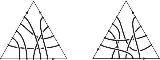
跳到论文正文
W Papers独立论文阅读器 arXiv:1003.5250 论文正文 计算阅读时间 · 0%
引用这篇论文根据当前论文元数据生成,正式投稿前建议核对。


License: arXiv.org perpetual non-exclusive license
arXiv:1003.5250v4 [math.GT] 17 Dec 2010

Quantum traces for representations of surface groups in SL2\mathrm{SL}_{2}Thanks: This research was partially supported by grants DMS-0632713 (Carleton Summer Mathematics Program) and DMS-0604866 from the National Science Foundation.

Francis Bonahon Address: Department of Mathematics, University of Southern California, Los Angeles CA 90089-2532, U.S.A. Email address: fbonahon@math.usc.edu and Helen Wong Address: Department of Mathematics, Carleton College, Northfield MN 55057, U.S.A. Email address: hwong@carleton.edu
Date: August 24, 2026
Abstract.

We consider two different quantizations of the character variety consisting of all representations of surface groups in PSL2\mathrm{PSL}_{2}. One is the skein algebra considered by Bullock-Frohman-Kania-Bartoszyńska, Przytycki-Sikora and Turaev. The other is the quantum Teichmüller space introduced by Chekhov-Fock and Kashaev. We construct a homomorphism from the skein algebra to the quantum Teichmüller space which, when restricted the classical case, corresponds to the equivalence between these two algebras through trace functions.

Let SS be an oriented surface of finite topological type. The goal of this paper is to establish a connection between two quantizations of the character variety

ℛSL2​(ℂ)(S)={r:π1(S)→SL2(ℂ)}//SL2(ℂ),\mathcal{R}_{\mathrm{SL}_{2}(\mathbb{C})}(S)=\{r\kern-3.0pt:\pi_{1}(S)\to\mathrm{SL}_{2}(\mathbb{C})\}/\kern-4.0pt/\mathrm{SL}_{2}(\mathbb{C}),

consisting of all group homomorphisms rr from the fundamental group π1​(S)\pi_{1}(S) to the Lie group SL2​(ℂ)\mathrm{SL}_{2}(\mathbb{C}), considered up to conjugation by elements of SL2​(ℂ)\mathrm{SL}_{2}(\mathbb{C}). The double bar indicates here that the quotient is taken in the algebraic geometric sense of geometric invariant theory.

The first quantization, introduced by D. Bullock, C. Frohman, J. Kania-Bartoszyńska [11], J. Przytycki, A. Sikora [39] and V. Turaev [43], uses the skein algebra 𝒮A​(S)\mathcal{S}^{A}(S) obtained by considering the vector space freely generated by all isotopy classes of framed links in S×[0,1]S\times[0,1], and then taking the quotient of this space under the Kauffman skein relation; see §3.1. What makes 𝒮A​(S)\mathcal{S}^{A}(S) a quantization of ℛSL2​(ℂ)​(S)\mathcal{R}_{\mathrm{SL}_{2}(\mathbb{C})}(S) is that, when A=−1A=-1, the skein algebra 𝒮−1​(S)\mathcal{S}^{-1}(S) has a natural identification with the commutative algebra of regular functions on ℛSL2​(ℂ)​(S)\mathcal{R}_{\mathrm{SL}_{2}(\mathbb{C})}(S) and that, as AA tends to −1-1, the lack of commutativity of 𝒮A​(S)\mathcal{S}^{A}(S) is infinitesimally measured by the Goldman-Weil-Petersson Poisson structure [25, 24, 38, 44] on ℛSL2​(ℂ)​(S)\mathcal{R}_{\mathrm{SL}_{2}(\mathbb{C})}(S); see [43]. There is a similar situation when A=+1A=+1, in which case 𝒮+1​(S)\mathcal{S}^{+1}(S) has a natural identification with a twisted version of ℛSL2​(ℂ)​(S)\mathcal{R}_{\mathrm{SL}_{2}(\mathbb{C})}(S); see §3.2.

The second quantization, with respect to the same Goldman-Weil-Petersson Poisson structure, is the quantum Teichmüller space 𝒯^Sq\widehat{\mathcal{T}}_{S}^{q} introduced by V. Fock and L. Chekhov [21, 16, 17] or, in a slightly different form, by R. Kashaev [30]; see also [5, 33, 27]. This quantization takes advantage of the fact that, if one restricts to matrices with real coefficients, a large subset of ℛSL2​(ℝ)​(S)\mathcal{R}_{\mathrm{SL}_{2}(\mathbb{R})}(S) with non-empty interior has a natural identification with the Teichmüller (or Fricke-Klein) space 𝒯⁡(S)\mathcal{T}(S), consisting of isotopy classes of all complete hyperbolic metrics on SS. Thurston [40] introduced for the Teichmüller space 𝒯⁡(S)\mathcal{T}(S) a set of coordinates, called shear coordinates, in which the Goldman-Weil-Petersson form is expressed in a particularly simple way. The quantum Teichmüller space is a quantization of 𝒯⁡(S)\mathcal{T}(S) that is based on these shear coordinates. This construction requires the surface to have at least one puncture.

A natural conjecture is that these two quantizations are “essentially equivalent”.

In the classical cases where q=1q=1 and A=±1A=\pm 1, the correspondence is relatively clear because of the identifications of 𝒮±1​(S)\mathcal{S}^{\pm 1}(S) and 𝒯^S1\widehat{\mathcal{T}}^{1}_{S} with algebras of functions on ℛSL2​(ℂ)​(S)\mathcal{R}_{\mathrm{SL}_{2}(\mathbb{C})}(S) and 𝒯⁡(S)\mathcal{T}(S). The only minor problem is that the functions considered in each case are not quite the same.

The correspondence between the skein algebra 𝒮±1​(S)\mathcal{S}^{\pm 1}(S) and the algebra of regular functions on ℛSL2​(ℂ)​(S)\mathcal{R}_{\mathrm{SL}_{2}(\mathbb{C})}(S) uses the trace functions TrK:ℛSL2​(ℂ)​(S)→ℝ\mathrm{Tr}_{K}\kern-3.0pt:\mathcal{R}_{\mathrm{SL}_{2}(\mathbb{C})}(S)\to\mathbb{R}, associated to all closed curves KK immersed in SS, which to a homomorphism r:π1​(S)→SL2​(ℂ)r\kern-3.0pt:\pi_{1}(S)\to\mathrm{SL}_{2}(\mathbb{C}) associates the trace of r​(K)∈SL2​(ℂ)r(K)\in\mathrm{SL}_{2}(\mathbb{C}) (see §§1.3 and 3.2 for technical details).

Shear coordinates depend on the choice of some topological information, namely on the choice of an ideal triangulation λ\lambda for the surface SS. For a real representation rm∈ℛSL2​(ℝ)​(S)r_{m}\in\mathcal{R}_{\mathrm{SL}_{2}(\mathbb{R})}(S) corresponding to a hyperbolic metric m∈𝒯⁡(S)m\in\mathcal{T}(S), the trace of rm​(K)r_{m}(K) can then be explicitly computed (see §3.2 for sign issues). This trace is actually expressed as a Laurent polynomial in the square roots of the shear coordinates of mm. This leads us to consider an algebra 𝒵^λ1\widehat{\mathcal{Z}}^{1}_{\lambda} consisting of rational fractions in the square roots of the shear coordinates, and to consider the algebra homomorphism

Trλ1:𝒮1​(S)→𝒵^λ1\mathrm{Tr}_{\lambda}^{1}\kern-3.0pt:\mathcal{S}^{1}(S)\to\widehat{\mathcal{Z}}^{1}_{\lambda}

which to [K]∈𝒮1​(S)[K]\in\mathcal{S}^{1}(S) associates the Laurent polynomial expressing the trace of rm​(K)r_{m}(K) in terms of the shear coordinates of m∈𝒯⁡(S)m\in\mathcal{T}(S).

In the quantum case, one similarly introduces a non-commutative algebra 𝒵^λω\widehat{\mathcal{Z}}^{\omega}_{\lambda} consisting of rational fractions in certain skew-commuting variables associated to the square roots of the shear coordinates. When q=ω4q=\omega^{4}, the quantum Teichmüller space 𝒯^Sq\widehat{\mathcal{T}}^{q}_{S} consists of those rational fractions in 𝒵^λω\widehat{\mathcal{Z}}^{\omega}_{\lambda} that involve only even powers of the variables. See §2.3 for details.

Theorem 1.

For A=ω−2A=\omega^{-2}, there is an algebra homomorphism

Trλω:𝒮A​(S)→𝒵^λω,\mathrm{Tr}_{\lambda}^{\omega}\kern-3.0pt:\mathcal{S}^{A}(S)\to\widehat{\mathcal{Z}}^{\omega}_{\lambda},

depending continuously on ω\omega in an appropriate sense, which corresponds to the above homomorphism Trλ1:𝒮1​(S)→𝒵λ1\mathrm{Tr}_{\lambda}^{1}\kern-3.0pt:\mathcal{S}^{1}(S)\to\mathcal{Z}^{1}_{\lambda} when ω=1\omega=1. In addition, the image Trλω​([K])∈𝒵^λω\mathrm{Tr}_{\lambda}^{\omega}([K])\in\widehat{\mathcal{Z}}^{\omega}_{\lambda} of every [K]∈𝒮A​(S)[K]\in\mathcal{S}^{A}(S) is a Laurent polynomial in the variables generating 𝒵^λω\widehat{\mathcal{Z}}^{\omega}_{\lambda}.

The homomorphism Trλω\mathrm{Tr}_{\lambda}^{\omega} is shown to be injective in Proposition 29.

A major step in the construction of the quantum Teichmüller space 𝒯^Sq\widehat{\mathcal{T}}_{S}^{q} is to make it independent of a choice of ideal triangulation. The homomorphism Trλω\mathrm{Tr}_{\lambda}^{\omega} of Theorem 1 is similarly independent of choices. Making sense of this statement uses work of C. Hiatt in [29] that extends to the square root set-up the original coordinate changes of Chekhov and Fock. More precisely, for any two ideal triangulations λ\lambda and λ′\lambda^{\prime} of the surface SS, Hiatt constructs a coordinate change isomorphism Θλ​λ′ω:𝒵^λ′ω→𝒵^λω\Theta_{\lambda\lambda^{\prime}}^{\omega}\kern-3.0pt:\widehat{\mathcal{Z}}^{\omega}_{\lambda^{\prime}}\to\widehat{\mathcal{Z}}^{\omega}_{\lambda} that restricts to the identity on 𝒯^Sq\widehat{\mathcal{T}}^{q}_{S}, considering the quantum Teichmüller space 𝒯^Sq\widehat{\mathcal{T}}^{q}_{S} as a subalgebra of both 𝒵^λω\widehat{\mathcal{Z}}^{\omega}_{\lambda} and 𝒵^λ′ω\widehat{\mathcal{Z}}^{\omega}_{\lambda^{\prime}}.

Theorem 2.

Given two ideal triangulations λ\lambda and λ′\lambda^{\prime} of the surface SS and given an element [K]∈𝒮A​(S)[K]\in\mathcal{S}^{A}(S) of the skein algebra of SS, the coordinate change map

Θλ​λ′ω:𝒵^λ′ω→𝒵^λω\Theta_{\lambda\lambda^{\prime}}^{\omega}\kern-3.0pt:\widehat{\mathcal{Z}}^{\omega}_{\lambda^{\prime}}\to\widehat{\mathcal{Z}}^{\omega}_{\lambda}

sends the Laurent polynomial Trλ′ω​(K)\mathrm{Tr}_{\lambda^{\prime}}^{\omega}(K) to the Laurent polynomial Trλω​(K)\mathrm{Tr}_{\lambda}^{\omega}(K).

While the proof of Theorem 1 is rather elaborate, the proof of Theorem 2 results from an easy application of the technology developed by Hiatt in [29].

Theorems 1 and 2 were conjectured in [21, 17], and proved for certain small surfaces in [18, 29]. Our proof is much more 3–dimensional than these earlier attempts. The technical challenge is to figure out a “good” way to order the non-commuting variables in each monomial of the Laurent polynomials considered; this is a classical problem in mathematical physics, where it is known as the search for a quantum ordering. Our solution is based on a careful control of the elevations of the strands of a link KK in S×[0,1]S\times[0,1], with respect to the [0,1][0,1] factor. The exposition that we give here is very computational, and involves a few miraculous identities (see in particular the proof of Proposition 26) that the reader may find somewhat frustrating. Recent conversations with C. Kassel seem to provide a more conceptual explanation for these identities, based on the fundamental representation of the dual SL2​(q)\mathrm{SL}_{2}(q) of the quantum group Uq​(sl2)\mathrm{U}_{q}(\mathrm{sl}_{2}); in particular, it might be possible to place our construction within the framework of [12, 13].

The motivation for this work finds its origins in the respective advantages and drawbacks of the two points of view on the character variety ℛSL2​(ℂ)​(S)\mathcal{R}_{\mathrm{SL}_{2}(\mathbb{C})}(S), and in their impact on the corresponding quantizations. The algebraic geometric approach of ℛSL2​(ℂ)​(S)\mathcal{R}_{\mathrm{SL}_{2}(\mathbb{C})}(S), based on trace functions, is very natural and its coordinate functions use only polynomials; however, it is hard to extract much information from this description. Conversely, the shear coordinates for the Teichmüller space are very concrete and geometric, but they also are less intrinsic (in particular for hyperbolic surfaces with infinite area, for which additional data is needed), do not behave well under the operation of restriction to subsurfaces, and are not defined for closed surfaces. The same features can be found at the quantum level. The skein algebra is very natural and occurs in many different contexts. However, its algebraic structure is quite difficult to handle at this point, except for small surfaces (see for instance [6, §3] for a discussion). Conversely, the quantum Teichmüller space has a very simple algebraic structure (it is a quantum torus), but it suffers from the lack of canonicity inherited from the classical shear coordinates.

One great advantage of the quantum Teichmüller space is that it has a very nice finite-dimensional representation theory, where an irreducible representation is essentially determined by a point in the character variety ℛPSL2​(ℂ)​(S)\mathcal{R}_{\mathrm{PSL}_{2}(\mathbb{C})}(S) [5, 2]. By composition with the trace homomorphism Trλω:𝒮A​(S)→𝒵^λω\mathrm{Tr}_{\lambda}^{\omega}\kern-3.0pt:\mathcal{S}^{A}(S)\to\widehat{\mathcal{Z}}^{\omega}_{\lambda} provided by Theorem 1, one obtains a wide family of finite-dimensional representations of the skein algebra 𝒮A​(S)\mathcal{S}^{A}(S). These representations behave well with respect to the action of the mapping class group, and a great feature of the corresponding machinery is that it works even for closed surfaces [6, 7, 8]. In particular, the results of the current paper represent a key technical step in a long-term program to study the representation theory of the skein algebra 𝒮A​(S)\mathcal{S}^{A}(S); see [6] for a discussion.

Acknowledgements. We are grateful to Adam Sikora for helping us sorting out our ideas in the classical case where A=±1A=\pm 1, and to Qingtao Chen for pointing out many misprints in the earlier versions of this paper.

1. The classical case

1.1. Ideal triangulations

The introduction was restricted to surfaces with no boundary, but it is convenient to allow boundary as well.

Let SS be an oriented punctured surface with boundary, obtained by removing finitely many points v1v_{1}, v2v_{2}, …, vpv_{p} from a compact connected oriented surface S¯\bar{S} with (possibly empty) boundary ∂S¯\partial\bar{S}. We require that each component of ∂S¯\partial\bar{S} contains at least one puncture viv_{i}, that there is at least one puncture, and that χ⁡(S)<d2\chi(S)<\frac{d}{2}, where χ⁡(S)\chi(S) is the Euler characteristic of SS and dd is the number of components of ∂S\partial S. These topological restrictions are equivalent to the existence of an ideal triangulation for SS, namely a triangulation of the closed surface S¯\bar{S} whose vertex set is exactly {v1,…,vp}\{v_{1},\dots,v_{p}\}. In particular, an ideal triangulation λ\lambda has n=−3​χ​(S)+2​dn=-3\chi(S)+2d edges and m=−2​χ​(S)+dm=-2\chi(S)+d faces. Its edges provide −3​χ​(S)+2​d-3\chi(S)+2d arcs λ1\lambda_{1}, …, λn\lambda_{n} in SS, going from puncture to puncture, which decompose the surface SS into −2​χ​(S)+d-2\chi(S)+d infinite triangles T1T_{1}, T2T_{2}, …, TmT_{m} whose vertices sit “at infinity” at the punctures. Note that dd of these λi\lambda_{i} are just the boundary components of SS.

1.2. The shear parameters

Suppose that we are given a positive weight Xi∈ℝ+X_{i}\in\mathbb{R}_{+} for each interior edge λi\lambda_{i} of the ideal triangulation λ\lambda. We can associate to this data a group homomorphism r:π1​(S)→PSL2​(ℝ)r\kern-3.0pt:\pi_{1}(S)\to\mathrm{PSL}_{2}(\mathbb{R}) as follows.

Lift the ideal triangulation λ\lambda to an ideal triangulation λ~\widetilde{\lambda} of the universal cover S~\widetilde{S}. We can then construct an orientation-preserving immersion f~:S~→ℍ2\widetilde{f}\kern-3.0pt:\widetilde{S}\to\mathbb{H}^{2} from S~\widetilde{S} to the hyperbolic plane ℍ2\mathbb{H}^{2} such that:

  1. (1)

    f~\widetilde{f} sends each face T~\widetilde{T} of λ~\widetilde{\lambda} to an ideal triangle of ℍ2\mathbb{H}^{2}, delimited by three disjoint geodesics and touching the circle at infinity ∂∞ℍ2\partial_{\infty}\mathbb{H}^{2} in 33 points;

  2. (2)

    when two faces T~\widetilde{T} and T~′\widetilde{T}^{\prime} meet along an edge λ~i\widetilde{\lambda}_{i} that projects to the edge λi\lambda_{i} of λ\lambda, then f~​(T~′)\widetilde{f}(\widetilde{T}^{\prime}) is obtained from f~​(T~)\widetilde{f}(\widetilde{T}) by performing a hyperbolic reflection across the geodesic f~​(λ~i)\widetilde{f}(\widetilde{\lambda}_{i}) followed by a hyperbolic translation of log⁡Xi\log X_{i} along the same geodesic f~​(λ~i)\widetilde{f}(\widetilde{\lambda}_{i}), if we orient f~​(λ~i)\widetilde{f}(\widetilde{\lambda}_{i}) by the boundary orientation of T~\widetilde{T}.

The immersion f~\widetilde{f} is easily constructed stepwise, and uniquely determined up to isotopy of S~\widetilde{S} respecting λ~\widetilde{\lambda}, once we have chosen the image of a single face of S~\widetilde{S}. In particular, the family of the ideal triangles f~​(T~)⊂ℍ2\widetilde{f}(\widetilde{T})\subset\mathbb{H}^{2} is unique up to an orientation-preserving isometry of ℍ2\mathbb{H}^{2}, namely up to composition by an element of PSL2​(ℝ)\mathrm{PSL}_{2}(\mathbb{R}).

From the construction, it is immediate that there is a unique group homomorphism r:π1​(S)→PSL2​(ℝ)r\kern-3.0pt:\pi_{1}(S)\to\mathrm{PSL}_{2}(\mathbb{R}) such that f~​(γ​T~)=r​(γ)​(T~)\widetilde{f}(\gamma\widetilde{T})=r(\gamma)(\widetilde{T}) for every face T~\widetilde{T} of λ~\widetilde{\lambda}. Since the family of the ideal triangles f~​(T~)\widetilde{f}(\widetilde{T}) is unique up to composition by an element of PSL2​(ℝ)\mathrm{PSL}_{2}(\mathbb{R}), rr is unique up to conjugation by an element of PSL2​(ℝ)\mathrm{PSL}_{2}(\mathbb{R}).

We say that r:π1​(S)→PSL2​(ℝ)r\kern-3.0pt:\pi_{1}(S)\to\mathrm{PSL}_{2}(\mathbb{R}) is associated to the shear parameters Xi∈ℝ+X_{i}\in\mathbb{R}_{+}.

1.3. The classical trace function

For a group homomorphism r:π1​(S)→PSL2​(ℝ)r\kern-3.0pt:\pi_{1}(S)\to\mathrm{PSL}_{2}(\mathbb{R}) and immersion f~:S~→ℍ2\widetilde{f}\kern-3.0pt:\widetilde{S}\to\mathbb{H}^{2} as above, consider a closed curve KK immersed in SS.

The fact that KK is immersed provides a natural lift r^​(K)∈SL2​(ℝ)\widehat{r}(K)\in\mathrm{SL}_{2}(\mathbb{R}) of r​(K)∈PSL2​(ℝ)r(K)\in\mathrm{PSL}_{2}(\mathbb{R}). Indeed, lift KK to an immersed path K~:[0,1]→S~\widetilde{K}\kern-3.0pt:[0,1]\to\widetilde{S}. Then r​(K)∈PSL2​(ℝ)r(K)\in\mathrm{PSL}_{2}(\mathbb{R}) is the unique orientation-preserving isometry of ℍ2\mathbb{H}^{2} sending the point f~∘K~​(0)∈ℍ2\widetilde{f}\circ\widetilde{K}(0)\in\mathbb{H}^{2} to f~∘K~​(1)\widetilde{f}\circ\widetilde{K}(1), and sending the vector (f~∘K~)′​(0)(\widetilde{f}\circ\widetilde{K})^{\prime}(0) to (f~∘K~)′​(1)(\widetilde{f}\circ\widetilde{K})^{\prime}(1). Now, for every t∈[0,1]t\in[0,1], we can consider the isometry r​(K)t∈PSL2​(ℝ)r(K)_{t}\in\mathrm{PSL}_{2}(\mathbb{R}) that sends the point f~∘K~​(0)∈ℍ2\widetilde{f}\circ\widetilde{K}(0)\in\mathbb{H}^{2} to f~∘K~​(t)\widetilde{f}\circ\widetilde{K}(t), and the vector (f~∘K~)′​(0)(\widetilde{f}\circ\widetilde{K})^{\prime}(0) to a positive real multiple of (f~∘K~)′​(t)(\widetilde{f}\circ\widetilde{K})^{\prime}(t). We now have a constructed a path t↦r​(K)t∈PSL2​(ℝ)t\mapsto r(K)_{t}\in\mathrm{PSL}_{2}(\mathbb{R}) that joins r​(K)0=Idℍ2r(K)_{0}=\mathrm{Id}_{\mathbb{H}^{2}} to r​(K)1=r⁡(K)r(K)_{1}=r(K). This path defines an element of the universal cover of PSL2​(ℝ)\mathrm{PSL}_{2}(\mathbb{R}), which projects to an element r^​(K)\widehat{r}(K) of the 2–fold cover SL2​(ℝ)\mathrm{SL}_{2}(\mathbb{R}) of PSL2​(ℝ)\mathrm{PSL}_{2}(\mathbb{R}).

We are particularly interested in the trace Tr​r^​(K)\mathrm{Tr}\,\widehat{r}(K) of r^​(K)∈SL2​(ℝ)\widehat{r}(K)\in\mathrm{SL}_{2}(\mathbb{R}). Note that, when KK is just a small circle bounding a disk embedded in SS, our designated lift r^​(K)\widehat{r}(K) is minus the identity matrix of SL2​(ℝ)\mathrm{SL}_{2}(\mathbb{R}), and Tr​r^​(K)=−2\mathrm{Tr}\,\widehat{r}(K)=-2.

If the homomorphism r:π1​(S)→PSL2​(ℝ)r\kern-3.0pt:\pi_{1}(S)\to\mathrm{PSL}_{2}(\mathbb{R}) is associated to shear parameters Xi∈ℝ+X_{i}\in\mathbb{R}_{+} assigned to the edges of the ideal triangulation λ\lambda, the construction of the map f~:S~→ℍ2\widetilde{f}\kern-3.0pt:\widetilde{S}\to\mathbb{H}^{2} and of the homomorphism rr is sufficiently explicit that r^​(K)∈SL2​(ℝ)\widehat{r}(K)\in\mathrm{SL}_{2}(\mathbb{R}) can be explicitly computed.

More precisely, suppose that KK transversely meets the edges λi1\lambda_{i_{1}}, λi2\lambda_{i_{2}}, …, λik\lambda_{i_{k}}, λik+1=λi1\lambda_{i_{k+1}}=\lambda_{i_{1}}, in this order. After crossing the edge λij\lambda_{i_{j}}, the curve KK enters a face TT of λ\lambda, which it exits through the edge λij+1\lambda_{i_{j+1}}. There are three possible choices for λij+1\lambda_{i_{j+1}}: it can be the edge immediately to the left as one enters TT through λij\lambda_{i_{j}}, the one immediately to the right, or it can be λij\lambda_{i_{j}} again if γ\gamma makes a U-turn in TT. In addition, because KK is immersed, we can measure the amount by which the tangent to KK turns between λij\lambda_{i_{j}} and λij+1\lambda_{i_{j+1}}. We then define a matrix MjM_{j} according to the various possible configurations.

If λij+1\lambda_{i_{j+1}} is the edge immediately to the left as one enters TT through λij\lambda_{i_{j}}, let tj∈ℤt_{j}\in\mathbb{Z} denote the number of full turns to the left that the tangent to KK makes between λij\lambda_{i_{j}} and λij+1\lambda_{i_{j+1}}, and let εj=(−1)tj=±1\varepsilon_{j}=(-1)^{t_{j}}=\pm 1. Here the topological number of turns tj∈ℤt_{j}\in\mathbb{Z} is measured so that tj=0t_{j}=0 when KK has no self-intersection between λij\lambda_{i_{j}} and λij+1\lambda_{i_{j+1}}; in fact, tjt_{j} has the same parity as the number of double points of KK between λij\lambda_{i_{j}} and λij+1\lambda_{i_{j+1}}. In this case, define

Mj=(εjεj0εj).M_{j}=\begin{pmatrix}\varepsilon_{j}&\varepsilon_{j}\\ 0&\varepsilon_{j}\end{pmatrix}.

For the analogous case where λij+1\lambda_{i_{j+1}} is the edge immediately to the right as one enters TT through λij\lambda_{i_{j}}, let again tj∈ℤt_{j}\in\mathbb{Z} denote the number of full turns to the left that the tangent to KK makes between λij\lambda_{i_{j}} and λij+1\lambda_{i_{j+1}}, and set εj=(−1)tj=±1\varepsilon_{j}=(-1)^{t_{j}}=\pm 1. Then define

Mj=(εj0εjεj).M_{j}=\begin{pmatrix}\varepsilon_{j}&0\\ \varepsilon_{j}&\varepsilon_{j}\end{pmatrix}.

In the case of a U-turn, where λij+1=λij\lambda_{i_{j+1}}=\lambda_{i_{j}}, let tj∈ℤt_{j}\in\mathbb{Z} be defined so that the tangent to KK makes 2​tj+12t_{j}+1 half-turns to the left between λij\lambda_{i_{j}} and λij+1\lambda_{i_{j+1}}, and set again εj=(−1)tj=±1\varepsilon_{j}=(-1)^{t_{j}}=\pm 1. Then define

Mj=(0εj−εj0).M_{j}=\begin{pmatrix}0&\varepsilon_{j}\\ -\varepsilon_{j}&0\end{pmatrix}.

Finally, having defined MjM_{j} in every case, consider for X>0X>0 the matrix

S⁡(X)=(X1200X−12).S(X)=\begin{pmatrix}X^{\frac{1}{2}}&0\\ 0&X^{-\frac{1}{2}}\end{pmatrix}.
Lemma 3.

Up to conjugation by an element of SL2​(ℝ)\mathrm{SL}_{2}(\mathbb{R}),

r^​(K)=S⁡(Xi1)​M1​S​(Xi2)​M2​…​S​(Xik)​Mk\widehat{r}(K)=S(X_{i_{1}})M_{1}S(X_{i_{2}})M_{2}\dots S(X_{i_{k}})M_{k}

where the matrices MjM_{j} and S⁡(Xij)S(X_{i_{j}}) are associated as above to the way the immersed curve KK crosses the edges of the ideal triangulation λ\lambda, and where Xi∈ℝ+X_{i}\in\mathbb{R}_{+} are the shear parameters defining the homomorphism r:π1​(S)→PSL2​(ℝ)r\kern-3.0pt:\pi_{1}(S)\to\mathrm{PSL}_{2}(\mathbb{R}).

Proof.

This is an easy exercise in hyperbolic geometry. See for instance Exercises 8.5–8.7 and 10.14 in [4]. ∎

1.4. State sums

As preparation for the quantum extension, we now give a state sum formula for the trace Tr​r^​(K)\mathrm{Tr}\,\widehat{r}(K) of the above element r^​(K)∈SL2​(ℝ)\widehat{r}(K)\in\mathrm{SL}_{2}(\mathbb{R}).

Let a state assign a sign s1s_{1}, s2s_{2}, …, sks_{k}, sk+1=s1∈{+,−}s_{k+1}=s_{1}\in\{+,-\} to each point where KK crosses an edge λij\lambda_{i_{j}} of λ\lambda, in this order. For j=1j=1, 22, …, kk, write the matrix MjM_{j} defined above as

Mj=(mj+⁣+mj+⁣−mj−⁣+mj−⁣−)M_{j}=\begin{pmatrix}m_{j}^{++}&m_{j}^{+-}\\ m_{j}^{-+}&m_{j}^{--}\end{pmatrix}

with mj±⁣±=0m_{j}^{\pm\pm}=0, +1+1 or −1-1. Then, the following formula immediately follows from Lemma 3 combined with elementary linear algebra.

Lemma 4.
Tr​r^​(K)=∑sm1s1​s2​m2s2​s3​…​mksk​s1​Xi1s12​Xi2s22​…​Xiksk2\mathrm{Tr}\,\widehat{r}(K)=\sum_{s}m_{1}^{s_{1}s_{2}}m_{2}^{s_{2}s_{3}}\dots m_{k}^{s_{k}s_{1}}X_{i_{1}}^{\frac{s_{1}}{2}}X_{i_{2}}^{\frac{s_{2}}{2}}\dots X_{i_{k}}^{\frac{s_{k}}{2}}

where the sum is over all possible states ss for KK and λ\lambda, and where in the exponents we identity the sign sj=±s_{j}=\pm to the number sj=±1s_{j}=\pm 1. ∎

2. The quantum Teichmüller space

2.1. The Chekhov-Fock algebra of an ideal triangulation

Let T1T_{1}, T2T_{2}, …, TmT_{m} be the faces of the ideal triangulation λ\lambda. Index the sides of each face TjT_{j} as λj​1\lambda_{j1}, λj​2\lambda_{j2}, λj​3\lambda_{j3}, in such a way that they occur in this order clockwise around TjT_{j}. We then associate to TjT_{j} a copy 𝒯Tjq\mathcal{T}_{T_{j}}^{q} of the triangle algebra, generated by three elements Xj​1X_{j1}, Xj​2X_{j2}, Xj​3X_{j3} and their inverses Xj​1−1X_{j1}^{-1}, Xj​2−1X_{j2}^{-1}, Xj​3−1X_{j3}^{-1}, and defined by the relations that Xj​1​Xj​2=q2​Xj​2​Xj​1X_{j1}X_{j2}=q^{2}X_{j2}X_{j1}, Xj​2​Xj​3=q2​Xj​3​Xj​2X_{j2}X_{j3}=q^{2}X_{j3}X_{j2} and Xj​3​Xj​1=q2​Xj​1​Xj​3X_{j3}X_{j1}=q^{2}X_{j1}X_{j3}. We here think of each generator Xj​aX_{ja} as being associated to the side λj​a\lambda_{ja} of TjT_{j}.

In the tensor product algebra 𝒯T1q⊗⋯⊗𝒯Tmq=⨂j=1m𝒯Tjq\mathcal{T}_{T_{1}}^{q}\otimes\dots\otimes\mathcal{T}_{T_{m}}^{q}=\bigotimes_{j=1}^{m}\mathcal{T}_{T_{j}}^{q}, we now associate to the edge λi\lambda_{i} of λ\lambda an element XiX_{i}, defined by:

  1. (1)

    Xi=Xj​a⊗Xk​bX_{i}=X_{ja}\otimes X_{kb} if λi\lambda_{i} separates two distinct faces TjT_{j} and TkT_{k}, and if Xj​a∈𝒯TjqX_{ja}\in\mathcal{T}_{T_{j}}^{q} and Xk​b∈𝒯TkqX_{kb}\in\mathcal{T}_{T_{k}}^{q} are the generators associated to the sides of TjT_{j} and TkT_{k} corresponding to λi\lambda_{i};

  2. (2)

    Xi=q−1​Xj​a​Xj​b=q​Xj​b​Xj​aX_{i}=q^{-1}X_{ja}X_{jb}=qX_{jb}X_{ja} if λi\lambda_{i} corresponds to two sides of the same face TjT_{j}, if Xj​aX_{ja}, Xj​b∈𝒯TjqX_{jb}\in\mathcal{T}_{T_{j}}^{q} are the generators associated to these two sides, and if Xj​aX_{ja} is associated to the side that comes first when going counterclockwise around their common vertex.

By convention, when describing an element Z1⊗⋯⊗ZmZ_{1}\otimes\dots\otimes Z_{m} of ⨂j=1m𝒯Tjq\bigotimes_{j=1}^{m}\mathcal{T}_{T_{j}}^{q}, we omit in the tensor product those ZjZ_{j} that are equal to the identity element 11 of 𝒯Tjq\mathcal{T}_{T_{j}}^{q}.

The Chekhov-Fock algebra of the ideal triangulation λ\lambda is the subalgebra 𝒯λq\mathcal{T}_{\lambda}^{q} of ⨂j=1m𝒯Tjq\bigotimes_{j=1}^{m}\mathcal{T}_{T_{j}}^{q} generated by the elements XiX_{i} associated as above to the edges of λ\lambda, and by their inverses Xi−1X_{i}^{-1}.

Note that Xi​Xj=q2​σi​j​Xj​XiX_{i}X_{j}=q^{2\sigma_{ij}}X_{j}X_{i} where the integers σi​j∈{0,±1,±2}\sigma_{ij}\in\{0,\pm 1,\pm 2\} are defined as follows: Let ai​ja_{ij} be the number of angular sectors delimited by λi\lambda_{i} and λj\lambda_{j} in the faces of λ\lambda, and with λi\lambda_{i} coming first counterclockwise; then σi​j=ai​j−aj​i\sigma_{ij}=a_{ij}-a_{ji}.

2.2. Coordinate changes between Chekhov-Fock algebras

As one switches from one ideal triangulation λ\lambda to another ideal triangulation λ′\lambda^{\prime}, the geometry of the Teichmüller space provides coordinate changes between the shear coordinates associated to λ\lambda and those associated to λ′\lambda^{\prime}. Because shear coordinates can be expressed as cross-ratios, one easily sees that these coordinate changes are given by rational maps.

In the quantum case, there is no underlying geometry to provide us with similar coordinate changes, and one has to find algebraic isomorphisms that have the required properties.

As in the classical case, these will involve rational fractions, and we consequently have to introduce the fraction division algebra 𝒯^λq\widehat{\mathcal{T}}_{\lambda}^{q} of the Chekhov-Fock algebra 𝒯λq\mathcal{T}_{\lambda}^{q}. Such a fraction division algebra exists because 𝒯λq\mathcal{T}_{\lambda}^{q} satisfies the so-called Ore Condition; see for instance [20, 31]. In practice, 𝒯^λq=ℂ​(X1,…,Xn)λq\widehat{\mathcal{T}}_{\lambda}^{q}=\mathbb{C}(X_{1},\dots,X_{n})_{\lambda}^{q} consists of non-commutative rational fractions in the variables X1X_{1}, …, XnX_{n} which are manipulated according to the qq-commutativity relations Xi​Xj=q2​σi​j​Xj​XiX_{i}X_{j}=q^{2\sigma_{ij}}X_{j}X_{i}.

L. Chekhov and V. Fock [21, 16, 17] (and R. Kashaev [30] in the context of length coordinates) construct such coordinate isomorphisms; see also [5, 33].

Theorem 5 (Chekhov-Fock, Kashaev).

There exists a family of algebra isomorphisms

Φλ​λ′q:𝒯^λ′q→𝒯^λq,\Phi_{\lambda\lambda^{\prime}}^{q}\kern-3.0pt:\widehat{\mathcal{T}}_{\lambda^{\prime}}^{q}\to\widehat{\mathcal{T}}_{\lambda}^{q},

defined for any two ideal triangulations λ\lambda, λ′\lambda^{\prime}, such that

Φλ​λ′′q=Φλ​λ′q∘Φλ′​λ′′q\Phi_{\lambda\lambda^{\prime\prime}}^{q}=\Phi_{\lambda\lambda^{\prime}}^{q}\circ\Phi_{\lambda^{\prime}\lambda^{\prime\prime}}^{q}

for any three ideal triangulations λ\lambda, λ′\lambda^{\prime} and λ′′\lambda^{\prime\prime}. ∎

This enables us to define the quantum Teichmüller space 𝒯^Sq\widehat{\mathcal{T}}_{S}^{q} of the punctured surface SS as the quotient

𝒯^Sq=∐λ𝒯^λq/∼\widehat{\mathcal{T}}_{S}^{q}=\coprod_{\lambda}\widehat{\mathcal{T}}_{\lambda}^{q}/\sim

of the disjoint union of the 𝒯^λq\widehat{\mathcal{T}}_{\lambda}^{q} of all ideal triangulations λ\lambda of SS, where the equivalence relation ∼\sim identifies 𝒯^λq\widehat{\mathcal{T}}_{\lambda}^{q} to 𝒯^λ′q\widehat{\mathcal{T}}_{\lambda^{\prime}}^{q} by the coordinate change isomorphism Φλ​λ′q\Phi_{\lambda\lambda^{\prime}}^{q}. Note that the property that Φλ​λ′′q=Φλ​λ′q∘Φλ′​λ′′q\Phi_{\lambda\lambda^{\prime\prime}}^{q}=\Phi_{\lambda\lambda^{\prime}}^{q}\circ\Phi_{\lambda^{\prime}\lambda^{\prime\prime}}^{q} is crucial to guarantee that ∼\sim is an equivalence relation. This property is much stronger than one could have thought at first glance, as indicated by the uniqueness result of [1].

Because the Φλ​λ′q\Phi_{\lambda\lambda^{\prime}}^{q} are algebra isomorphisms, the quantum Teichmüller space 𝒯^Sq\widehat{\mathcal{T}}_{S}^{q} inherits an algebra structure from the 𝒯^λq\widehat{\mathcal{T}}_{\lambda}^{q}.

2.3. The Chekhov-Fock square root algebra

The formulas of Lemma 4 involve square roots of shear coordinates. This lead us to consider formal square roots Zi=Xi12Z_{i}=X_{i}^{\frac{1}{2}} of the generators of the Chekhov-Fock algebra 𝒯λq\mathcal{T}_{\lambda}^{q}.

In practice, one just considers the Chekhov-Fock algebra 𝒯λω\mathcal{T}_{\lambda}^{\omega} associated to a fourth root ω=q14\omega=q^{\frac{1}{4}} of qq. To avoid confusion, we denote by ZiZ_{i} the generator of 𝒯λω\mathcal{T}_{\lambda}^{\omega} associated to the edge λi\lambda_{i} of λ\lambda while, as before, XiX_{i} is the generator of 𝒯λq\mathcal{T}_{\lambda}^{q} associated to the same λi\lambda_{i}. Then, there exists an injective algebra homomorphism 𝒯λq→𝒯λω\mathcal{T}_{\lambda}^{q}\to\mathcal{T}_{\lambda}^{\omega} associating the element Zi2Z_{i}^{2} to the generator XiX_{i}, so that we can consider 𝒯λq\mathcal{T}_{\lambda}^{q} as a subalgebra of 𝒯λω\mathcal{T}_{\lambda}^{\omega}. This also induces a similar inclusion 𝒯^λq⊂𝒯^λω\widehat{\mathcal{T}}_{\lambda}^{q}\subset\widehat{\mathcal{T}}_{\lambda}^{\omega} between the corresponding fraction division algebras.

In the classical case, the coordinate changes between square roots of shear coordinates are not as nice as those between shear coordinates, because they are not rational anymore. The same consequently holds in the quantum setup. However, there is a subalgebra of the algebra 𝒯λω\mathcal{T}_{\lambda}^{\omega} which is better behaved with respect to coordinate changes.

A monomial Z1k1​Z2k2​…​ZnknZ_{1}^{k_{1}}Z_{2}^{k_{2}}\dots Z_{n}^{k_{n}} in the generators ZiZ_{i} of 𝒯λω\mathcal{T}_{\lambda}^{\omega} is said to be balanced if, for every triangle face TjT_{j} of λ\lambda, the exponents kik_{i} of the generators ZiZ_{i} associated to the three sides of TjT_{j} add up to an even number. (When the same edge λi\lambda_{i} corresponds to two distinct sides of TjT_{j}, the exponent kik_{i} is counted twice in the sum.) This is equivalent to the property that there exists a homology class α∈H1​(S,ℤ2)\alpha\in H_{1}(S;\mathbb{Z}_{2}) such that the class of the exponent kik_{i} in ℤ2\mathbb{Z}_{2} is equal to the algebraic intersection number of α\alpha with the edge λi\lambda_{i}. In this case, we will say that the monomial Z1k1​Z2k2​…​ZnknZ_{1}^{k_{1}}Z_{2}^{k_{2}}\dots Z_{n}^{k_{n}} is α\alpha–balanced.

In the Chekhov-Fock algebra 𝒯λω\mathcal{T}_{\lambda}^{\omega}, let 𝒵λω\mathcal{Z}^{\omega}_{\lambda} denote the linear subspace generated by all balanced monomials. Note that it splits as a direct sum

𝒵λω=⨁α∈H1​(S,ℤ2)𝒵λω​(α)\mathcal{Z}^{\omega}_{\lambda}=\bigoplus_{\alpha\in H_{1}(S,\mathbb{Z}_{2})}\mathcal{Z}^{\omega}_{\lambda}(\alpha)

where 𝒵λω​(α)\mathcal{Z}^{\omega}_{\lambda}(\alpha) denotes the linear subspace generated by all α\alpha–balanced monomials. The product of an element of 𝒵λω​(α)\mathcal{Z}^{\omega}_{\lambda}(\alpha) with an element of 𝒵λω​(β)\mathcal{Z}^{\omega}_{\lambda}(\beta) belongs to 𝒵λω​(α+β)\mathcal{Z}^{\omega}_{\lambda}(\alpha+\beta), so that 𝒵λω\mathcal{Z}^{\omega}_{\lambda} is a subalgebra of 𝒯λω\mathcal{T}_{\lambda}^{\omega}. We will refer to 𝒵λω\mathcal{Z}^{\omega}_{\lambda} as the Chekhov-Fock square root algebra of the ideal triangulation λ\lambda.

Note that 𝒵λω​(0)\mathcal{Z}^{\omega}_{\lambda}(0) coincides with the subalgebra 𝒯λq⊂𝒯λω\mathcal{T}_{\lambda}^{q}\subset\mathcal{T}_{\lambda}^{\omega} generated by the Zi2=XiZ_{i}^{2}=X_{i}.

In the fraction algebra 𝒯^λω\widehat{\mathcal{T}}_{\lambda}^{\omega}, we now consider the subset 𝒵^λω\widehat{\mathcal{Z}}^{\omega}_{\lambda} consisting of all fractions P/QP/Q where P∈𝒵λωP\in\mathcal{Z}^{\omega}_{\lambda} and Q∈𝒵λω​(0)=𝒯λqQ\in\mathcal{Z}^{\omega}_{\lambda}(0)=\mathcal{T}_{\lambda}^{q}. One easily checks that 𝒵^λω\widehat{\mathcal{Z}}^{\omega}_{\lambda} is a subalgebra of 𝒯^λω\widehat{\mathcal{T}}_{\lambda}^{\omega}. It also contains the Chekhov-Fock fraction algebra 𝒯^λq\widehat{\mathcal{T}}_{\lambda}^{q}.

In [29], Chris Hiatt extends the Chekhov-Fock coordinate change isomorphism Φλ​λ′:𝒯^λ′q→𝒯^λq\Phi_{\lambda\lambda^{\prime}}\kern-3.0pt:\widehat{\mathcal{T}}_{\lambda^{\prime}}^{q}\to\widehat{\mathcal{T}}_{\lambda}^{q} of Theorem 5 to the Chekhov-Fock square root algebra 𝒵λω\mathcal{Z}^{\omega}_{\lambda}.

Theorem 6 (Hiatt).

When q=ω4q=\omega^{4}, there exists for any two ideal triangulations λ\lambda, λ′\lambda^{\prime} an algebra isomorphism

Θλ​λ′ω:𝒵^λ′ω→𝒵^λω\Theta_{\lambda\lambda^{\prime}}^{\omega}\kern-3.0pt:\widehat{\mathcal{Z}}^{\omega}_{\lambda^{\prime}}\to\widehat{\mathcal{Z}}^{\omega}_{\lambda}

extending the Chekhov-Fock coordinate change isomorphism Φλ​λ′:𝒯^λ′q→𝒯^λq\Phi_{\lambda\lambda^{\prime}}\kern-3.0pt:\widehat{\mathcal{T}}_{\lambda^{\prime}}^{q}\to\widehat{\mathcal{T}}_{\lambda}^{q}. In addition, Θλ​λ′′ω=Θλ​λ′ω∘Θλ′​λ′′ω\Theta_{\lambda\lambda^{\prime\prime}}^{\omega}=\Theta_{\lambda\lambda^{\prime}}^{\omega}\circ\Theta_{\lambda^{\prime}\lambda^{\prime\prime}}^{\omega} for any three ideal triangulations λ\lambda, λ′\lambda^{\prime} and λ′′\lambda^{\prime\prime}.

Proof.

Hiatt does not quite prove the result in this form, so we need to explain how to obtain it from [29, §§6–7].

For every α∈H1​(S,ℤ2)\alpha\in H_{1}(S;\mathbb{Z}_{2}), let 𝒵^λω​(α)\widehat{\mathcal{Z}}^{\omega}_{\lambda}(\alpha) consist of all fractions P/QP/Q where P∈𝒵λω​(α)P\in\mathcal{Z}^{\omega}_{\lambda}(\alpha) and Q∈𝒵λω​(0)=𝒯λqQ\in\mathcal{Z}^{\omega}_{\lambda}(0)=\mathcal{T}_{\lambda}^{q}, so that

𝒵^λω=⨁α∈H1​(S,ℤ2)𝒵^λω​(α).\widehat{\mathcal{Z}}^{\omega}_{\lambda}=\bigoplus_{\alpha\in H_{1}(S,\mathbb{Z}_{2})}\widehat{\mathcal{Z}}^{\omega}_{\lambda}(\alpha).

Hiatt constructs in [29, §6] a linear map Θλ​λ′ω:𝒵^λ′ω​(α)→𝒵^λω​(α)\Theta_{\lambda\lambda^{\prime}}^{\omega}\kern-3.0pt:\widehat{\mathcal{Z}}^{\omega}_{\lambda^{\prime}}(\alpha)\to\widehat{\mathcal{Z}}^{\omega}_{\lambda}(\alpha). The construction of this map in [29] a priori depends on the choice of an 1–dimensional submanifold KK immersed in SS and representing the homology class α∈H1​(S,ℤ2)\alpha\in H_{1}(S;\mathbb{Z}_{2}). However, it easily follows from [29, Lemma 17] that this map depends only on α\alpha.

Linearly extend these maps Θλ​λ′ω:𝒵^λ′ω​(α)→𝒵^λω​(α)\Theta_{\lambda\lambda^{\prime}}^{\omega}\kern-3.0pt:\widehat{\mathcal{Z}}^{\omega}_{\lambda^{\prime}}(\alpha)\to\widehat{\mathcal{Z}}^{\omega}_{\lambda}(\alpha) to a linear map Θλ​λ′ω:𝒵^λ′ω→𝒵^λω\Theta_{\lambda\lambda^{\prime}}^{\omega}\kern-3.0pt:\widehat{\mathcal{Z}}^{\omega}_{\lambda^{\prime}}\to\widehat{\mathcal{Z}}^{\omega}_{\lambda}.

To show that this is an algebra homomorphism we need to check that, for every A∈𝒵^λ′ω​(α)A\in\widehat{\mathcal{Z}}^{\omega}_{\lambda^{\prime}}(\alpha) and B∈𝒵^λ′ω​(β)B\in\widehat{\mathcal{Z}}^{\omega}_{\lambda^{\prime}}(\beta), Θλ​λ′ω​(A)​Θλ​λ′ω​(B)=Θλ​λ′ω​(A​B)\Theta_{\lambda\lambda^{\prime}}^{\omega}(A)\Theta_{\lambda\lambda^{\prime}}^{\omega}(B)=\Theta_{\lambda\lambda^{\prime}}^{\omega}(AB) in 𝒵^λω​(α+β)\widehat{\mathcal{Z}}^{\omega}_{\lambda}(\alpha+\beta). This is an immediate consequence of [29, Sublemma 19] and of the construction of Θλ​λ′ω\Theta_{\lambda\lambda^{\prime}}^{\omega}.

The fact that the restriction of Θλ​λ′ω\Theta_{\lambda\lambda^{\prime}}^{\omega} to 𝒵^λ′ω​(0)=𝒯^λ′q\widehat{\mathcal{Z}}^{\omega}_{\lambda^{\prime}}(0)=\widehat{\mathcal{T}}_{\lambda^{\prime}}^{q} coincides with Φλ​λ′q\Phi_{\lambda\lambda^{\prime}}^{q} immediately follows from its construction in [29]. The property that Θλ​λ′′ω=Θλ​λ′ω∘Θλ′​λ′′ω\Theta_{\lambda\lambda^{\prime\prime}}^{\omega}=\Theta_{\lambda\lambda^{\prime}}^{\omega}\circ\Theta_{\lambda^{\prime}\lambda^{\prime\prime}}^{\omega} is proved in [29, Theorem 25]. ∎

Remark 7.

For A∈𝒵^λωA\in\widehat{\mathcal{Z}}^{\omega}_{\lambda}, the operator point of view of [21, 16, 17] much more easily provides a natural square root Θλ​λ′ω​(A)\Theta_{\lambda\lambda^{\prime}}^{\omega}(A) of Φλ​λ′q​(A2)\Phi_{\lambda\lambda^{\prime}}^{q}(A^{2}). The real content of Theorem 6 is that this square root can be expressed as a rational fraction in the generators Zi=Xi12Z_{i}=X_{i}^{\frac{1}{2}}. The restriction to 𝒵^λ′ω\widehat{\mathcal{Z}}^{\omega}_{\lambda^{\prime}} is here crucial.

3. The skein algebra

3.1. Links and skeins

We begin with the framed link algebra 𝒦⁡(S)\mathcal{K}(S). This is the vector space (over ℂ\mathbb{C}, say) freely generated by the isotopy classes of (unoriented) 1–dimensional framed submanifolds K⊂S×[0,1]K\subset S\times[0,1] such that:

  1. (1)

    ∂K=K∩∂(S×[0,1])\partial K=K\cap\partial(S\times[0,1]) consists of finitely many points in (∂S)×[0,1](\partial S)\times[0,1];

  2. (2)

    at every point of ∂K\partial K, the framing is vertical, namely parallel to the [0,1][0,1] factor, and points in the direction of 11;

  3. (3)

    for every component kk of ∂S\partial S, the points of ∂K\partial K that are in k×[0,1]k\times[0,1] sit at different elevations, namely have different [0,1][0,1]–coordinates.

An isotopy of such framed submanifolds of course is required to respect all three conditions. The third condition will turn out to be crucial for our analysis.

Perhaps we should have begun by specifying what we mean by a framing for KK. For us here, a framing is a continuous choice of a vector transverse to KK at each point of KK.

The vector space 𝒦⁡(S)\mathcal{K}(S) can be endowed with a multiplication, where the product of K1K_{1} and K2K_{2} is defined by the framed link K⊂S×[0,1]K\subset S\times[0,1] that is the union of K1K_{1} rescaled in S×[0,12]S\times[0,\frac{1}{2}] and K2K_{2} rescaled in S×[12,1]S\times[\frac{1}{2},1]. In other words, the product K1​K2K_{1}K_{2} is defined by superposition of the framed links K1K_{1} and K2K_{2}. Note that this superposition operation is compatible with isotopies, and therefore provides a well-defined algebra structure on 𝒦⁡(S)\mathcal{K}(S).

Three links K1K_{1}, K0K_{0} and K∞K_{\infty} in S×[0,1]S\times[0,1] form a Kauffman triple if the only place where they differ is above a small disk in SS, where they are as represented in Figure 1 (as seen from above) and where the framing is vertical and pointing upwards (namely the framing is parallel to the [0,1][0,1] factor and points towards 11).

The Kauffman skein algebra 𝒮A​(S)\mathcal{S}^{A}(S) is the quotient of the framed link algebra 𝒦⁡(K)\mathcal{K}(K) by the two-sided ideal generated by all elements K1−A−1​K0−A​K∞K_{1}-A^{-1}K_{0}-AK_{\infty} as (K1,K0,K∞)(K_{1},K_{0},K_{\infty}) ranges over all Kauffman triples. The superposition operation descends to a multiplication in 𝒮A​(S)\mathcal{S}^{A}(S), endowing 𝒮A​(S)\mathcal{S}^{A}(S) with the structure of an algebra. The class [∅][\varnothing] of the empty link is an identity element in 𝒮A​(S)\mathcal{S}^{A}(S), and is usually denoted by 11.

An element [K]∈𝒮A​(S)[K]\in\mathcal{S}^{A}(S), represented by a framed link K∈𝒦⁡(S)K\in\mathcal{K}(S), is a skein in SS. The construction is defined to ensure that the skein relation

[K1]=A−1​[K0]+A⁡[K∞][K_{1}]=A^{-1}[K_{0}]+A[K_{\infty}]

holds in 𝒮A​(S)\mathcal{S}^{A}(S) for every Kauffman triple (K1,K0,K∞)(K_{1},K_{0},K_{\infty}).

Refer to caption        K0K_{0}   K1K_{1}              K∞K_{\infty}               

[K1]=A−1​[K0]+A⁡[K∞][K_{1}]=A^{-1}[K_{0}]+A[K_{\infty}]
Figure 1. The skein relation

3.2. The classical cases 𝐀=±𝟏\mathbf{A=\pm 1}

In [9, 10, 11, 39], D. Bullock, C. Frohman, J. Kania-Bartoszyńska, J. Przytycki and A. Sikora observe that there is a strong connection between the skein algebra with A=−1A=-1 and the character variety

ℛSL2​(ℂ)(S)={group homomorphisms r:π1(S)→SL2(ℂ)}//SL2(ℂ).\mathcal{R}_{\mathrm{SL}_{2}(\mathbb{C})}(S)=\{\text{group homomorphisms }r\kern-3.0pt:\pi_{1}(S)\to\mathrm{SL}_{2}(\mathbb{C})\}/\kern-4.0pt/\mathrm{SL}_{2}(\mathbb{C}).

The quotient is under the action by conjugation, and should be understood in the sense of geometric invariant theory [36] to avoid pathologies near the reducible homomorphisms.

Note that, for every AA, there is a unique algebra homomorphism 𝒮A​(S)→ℂ\mathcal{S}^{A}(S)\to\mathbb{C} that sends each non-empty skein [K]∈𝒮A​(S)[K]\in\mathcal{S}^{A}(S) to 00 and sends the empty skein [∅]=1[\varnothing]=1 to 11. This homomorphism is the trivial homomorphism 𝒮A​(S)→ℂ\mathcal{S}^{A}(S)\to\mathbb{C}.

Theorem 8 ([9, 10, 11, 39]).

Assume that the surface SS has no boundary (but is still allowed to have punctures), and consider the skein algebra 𝒮−1​(S)\mathcal{S}^{-1}(S) corresponding to A=−1A=-1. Every group homomorphism r:π1​(S)→SL2​(ℂ)r\kern-3.0pt:\pi_{1}(S)\to\mathrm{SL}_{2}(\mathbb{C}) defines a unique non-trivial algebra homomorphism Tr:𝒮−1​(S)→ℂT_{r}\kern-3.0pt:\mathcal{S}^{-1}(S)\to\mathbb{C} by the property that

Tr​([K])=−Tr​r​(K)T_{r}([K])=-\mathrm{Tr}\,r(K)

for every connected skein [K]∈𝒮−1​(S)[K]\in\mathcal{S}^{-1}(S).

Conversely, every non-trivial algebra homomorphism T:𝒮−1​(S)→ℂT\kern-3.0pt:\mathcal{S}^{-1}(S)\to\mathbb{C} is associated to a unique r∈ℛSL2​(ℂ)​(S)r\in\mathcal{R}_{\mathrm{SL}_{2}(\mathbb{C})}(S) in this way. ∎

Note that the definition of r​(K)∈SL2​(ℂ)r(K)\in\mathrm{SL}_{2}(\mathbb{C}) implicitly supposes the choice of an orientation for the closed curve KK. However, reversing this orientation replaces r⁡(K)r(K) by its inverse, and leaves the trace Tr​r​(K)\mathrm{Tr}\,r(K) unchanged.

There is a similar result for the other case where the skein algebra 𝒮A​(S)\mathcal{S}^{A}(S) is commutative, corresponding to A=1A=1. This statement uses the correspondence 𝒮A​(S)≅𝒮−A​(S)\mathcal{S}^{A}(S)\cong\mathcal{S}^{-A}(S) established by J. Barrett [3], and requires the use of spin structures.

Let Spin⁡(S)\mathrm{Spin}(S) be the set of isotopy classes of spin structures on SS or, equivalently, the set of isotopy classes of spin structures on S×[0,1]S\times[0,1]. Any two elements of Spin⁡(S)\mathrm{Spin}(S) differ by an obstruction in H1​(S,ℤ2)H^{1}(S;\mathbb{Z}_{2}), so that there is an action of H1​(S,ℤ2)H^{1}(S;\mathbb{Z}_{2}) on Spin⁡(S)\mathrm{Spin}(S).

Similarly, the cohomology group H1​(S,ℤ2)H^{1}(S;\mathbb{Z}_{2}) acts on ℛSL2​(ℂ)​(S)\mathcal{R}_{\mathrm{SL}_{2}(\mathbb{C})}(S) by the property that, if α∈H1​(S,ℤ2)\alpha\in H^{1}(S;\mathbb{Z}_{2}) and r:π1​(S)→SL2​(ℂ)r\kern-3.0pt:\pi_{1}(S)\to\mathrm{SL}_{2}(\mathbb{C}), then α​r∈ℛSL2​(ℂ)​(S)\alpha r\in\mathcal{R}_{\mathrm{SL}_{2}(\mathbb{C})}(S) associates (−1)α⁡(γ)​r​(γ)∈SL2​(ℂ)(-1)^{\alpha(\gamma)}r(\gamma)\in\mathrm{SL}_{2}(\mathbb{C}) to γ∈π1​(S)\gamma\in\pi_{1}(S). Note that the quotient of ℛSL2​(ℂ)​(S)\mathcal{R}_{\mathrm{SL}_{2}(\mathbb{C})}(S) under this action of H1​(S,ℤ2)H^{1}(S;\mathbb{Z}_{2}) is just the character variety

ℛPSL2​(ℂ)(S)={group homomorphisms r:π1(S)→PSL2(ℂ)}//PSL2(ℂ)\mathcal{R}_{\mathrm{PSL}_{2}(\mathbb{C})}(S)=\{\text{group homomorphisms }r\kern-3.0pt:\pi_{1}(S)\to\mathrm{PSL}_{2}(\mathbb{C})\}/\kern-4.0pt/\mathrm{PSL}_{2}(\mathbb{C})

of homomorphisms valued in PSL2​(ℂ)\mathrm{PSL}_{2}(\mathbb{C}) instead of SL2​(C)\mathrm{SL}_{2}(C). (It is here important that SS is non-compact so that, because the fundamental π1​(S)\pi_{1}(S) is free, every homomorphism π1→PSL2​(ℂ)\pi_{1}\to\mathrm{PSL}_{2}(\mathbb{C}) lifts to SL2​(ℂ)\mathrm{SL}_{2}(\mathbb{C}).)

We can then combine these actions of H1​(S,ℤ2)H^{1}(S;\mathbb{Z}_{2}) on Spin⁡(S)\mathrm{Spin}(S) and ℛSL2​(ℂ)​(S)\mathcal{R}_{\mathrm{SL}_{2}(\mathbb{C})}(S), and consider the twisted product

ℛPSL2​(ℂ)Spin​(S)=ℛPSL2​(ℂ)​(S)​×~​Spin​(S)=(ℛSL2​(ℂ)​(S)×Spin⁡(S))/H1​(S,ℤ2).\mathcal{R}_{\mathrm{PSL}_{2}(\mathbb{C})}^{\mathrm{Spin}}(S)=\mathcal{R}_{\mathrm{PSL}_{2}(\mathbb{C})}(S)\widetilde{\times}\,\mathrm{Spin}(S)=\bigl(\mathcal{R}_{\mathrm{SL}_{2}(\mathbb{C})}(S)\times\mathrm{Spin}(S)\bigr)/H^{1}(S;\mathbb{Z}_{2}).

Note that, just like ℛSL2​(ℂ)​(S)\mathcal{R}_{\mathrm{SL}_{2}(\mathbb{C})}(S), this twisted product ℛPSL2​(ℂ)Spin​(S)\mathcal{R}_{\mathrm{PSL}_{2}(\mathbb{C})}^{\mathrm{Spin}}(S) is a finite cover of ℛPSL2​(ℂ)​(S)\mathcal{R}_{\mathrm{PSL}_{2}(\mathbb{C})}(S) with fiber H1​(S,ℤ2)≅Spin⁡(S)H^{1}(S;\mathbb{Z}_{2})\cong\mathrm{Spin}(S).

If σ∈Spin⁡(S)\sigma\in\mathrm{Spin}(S) is a spin structure and KK is a framed knot in S×[0,1]S\times[0,1], the monodromy of the framing of KK with respect to σ\sigma defines an element σ⁡(K)∈ℤ2\sigma(K)\in\mathbb{Z}_{2}. If, in addition, we are given a group homomorphism r:π1​(S)→SL2​(ℂ)r\kern-3.0pt:\pi_{1}(S)\to\mathrm{SL}_{2}(\mathbb{C}), we can consider the element T(r,σ)​(K)=(−1)σ⁡(K)​Tr​r​(K)T_{(r,\sigma)}(K)=(-1)^{\sigma(K)}\mathrm{Tr}\,r(K). Note that T(r,σ)​(K)T_{(r,\sigma)}(K) is invariant under the action of H1​(S,ℤ2)H^{1}(S;\mathbb{Z}_{2}) on the pair (r,σ)(r,\sigma), and therefore depends only on the class of (r,σ)(r,\sigma) in ℛPSL2​(ℂ)Spin​(S)\mathcal{R}_{\mathrm{PSL}_{2}(\mathbb{C})}^{\mathrm{Spin}}(S).

Theorem 9.

Assume that the surface SS has no boundary (but is still allowed to have punctures), and consider the skein algebra 𝒮1​(S)\mathcal{S}^{1}(S) corresponding to A=+1A=+1. Every group homomorphism r:π1​(S)→SL2​(ℂ)r\kern-3.0pt:\pi_{1}(S)\to\mathrm{SL}_{2}(\mathbb{C}) and spin structure σ∈Spin⁡(S)\sigma\in\mathrm{Spin}(S) define a unique algebra homomorphism T(r,σ):𝒮1​(S)→ℂT_{(r,\sigma)}\kern-3.0pt:\mathcal{S}^{1}(S)\to\mathbb{C} by the property that

T(r,σ)​([K])=(−1)σ⁡(K)​Tr​r​(K)T_{(r,\sigma)}([K])=(-1)^{\sigma(K)}\mathrm{Tr}\,r(K)

for every connected skein [K]∈𝒮1​(S)[K]\in\mathcal{S}^{1}(S). This homomorphism T(r,σ)T_{(r,\sigma)} is non-trivial and depends only on the class of (r,σ)(r,\sigma) in ℛPSL2​(ℂ)Spin​(S)\mathcal{R}_{\mathrm{PSL}_{2}(\mathbb{C})}^{\mathrm{Spin}}(S).

Conversely, every non-trivial algebra homomorphism T:𝒮1​(S)→ℂT\kern-3.0pt:\mathcal{S}^{1}(S)\to\mathbb{C} is associated to a unique element (r,σ)∈ℛPSL2​(ℂ)Spin​(S)(r,\sigma)\in\mathcal{R}_{\mathrm{PSL}_{2}(\mathbb{C})}^{\mathrm{Spin}}(S) in this way.

Proof.

Fix a spin structure σ∈Spin⁡(S)\sigma\in\mathrm{Spin}(S). Then Barrett [3] defines an algebra isomorphism 𝒮1​(S)→𝒮−1​(S)\mathcal{S}^{1}(S)\to\mathcal{S}^{-1}(S) associating (−1)k+σ⁡(K)​[K]∈𝒮−1​(S)(-1)^{k+\sigma(K)}[K]\in\mathcal{S}^{-1}(S) to every skein [K]∈𝒮1​(S)[K]\in\mathcal{S}^{1}(S) represented by a link KK with kk components (see [39, §2] for a proof that this is an algebra homomorphism). The result then immediately follows by combining Theorem 8 with this correspondence. ∎

To connect the set-up of §1.3 to Theorem 9, consider a hyperbolic metric m∈𝒯⁡(S)m\in\mathcal{T}(S). It is convenient to move to a 3–dimensional framework, by extending m∈𝒯⁡(S)m\in\mathcal{T}(S) to a 3–dimensional hyperbolic metric on a small thickening S×(0,1)S\times(0,1) of S=S×{12}S=S\times\{\frac{1}{2}\}. We can even consider the more general case of a hyperbolic metric mm on S×(0,1)S\times(0,1), not necessarily complete. Classically, this hyperbolic metric mm on S×(0,1)S\times(0,1) has a well-defined monodromy homomorphism r∈ℛPSL2​(ℂ)​(S)r\in\mathcal{R}_{\mathrm{PSL}_{2}(\mathbb{C})}(S). What seems less well-known is that mm provides additional spin information, and uniquely determines an element of the twisted product ℛPSL2​(ℂ)Spin​(S)=ℛPSL2​(ℂ)​(S)​×~​Spin​(S)\mathcal{R}_{\mathrm{PSL}_{2}(\mathbb{C})}^{\mathrm{Spin}}(S)=\mathcal{R}_{\mathrm{PSL}_{2}(\mathbb{C})}(S)\widetilde{\times}\,\mathrm{Spin}(S).

A spin structure σ∈Spin⁡(S)\sigma\in\mathrm{Spin}(S) specifies a way to lift the monodromy homomorphism r:π1​(S)→PSL2​(ℂ)r\kern-3.0pt:\pi_{1}(S)\to\mathrm{PSL}_{2}(\mathbb{C}) to a homomorphism rσ:π1​(S)→SL2​(ℂ)r_{\sigma}\kern-3.0pt:\pi_{1}(S)\to\mathrm{SL}_{2}(\mathbb{C}) as follows. For this, first extend σ\sigma to a spin structure on the thickened surface S×(0,1)S\times(0,1). Then consider a developing map for the metric mm, namely an isometric immersion f~:S~×(0,1)→ℍ3\widetilde{f}\kern-3.0pt:\widetilde{S}\times(0,1)\to\mathbb{H}^{3} from the universal cover S~×(0,1)\widetilde{S}\times(0,1) to the hyperbolic space ℍ3\mathbb{H}^{3} that is equivariant with respect to the monodromy r:π1​(S)→PSL2​(ℂ)r\kern-3.0pt:\pi_{1}(S)\to\mathrm{PSL}_{2}(\mathbb{C}).

Represent [γ]∈π1​(S)=π1​(S,x0)[\gamma]\in\pi_{1}(S)=\pi_{1}(S;x_{0}) by a path γ:[0,1]→S×(0,1)\gamma\kern-3.0pt:[0,1]\to S\times(0,1) with γ⁡(0)=γ⁡(1)=x0\gamma(0)=\gamma(1)=x_{0}. Pick an arbitrary orthonormal frame F⁡(t)F(t) at each γ⁡(t)\gamma(t), depending continuously on tt and such that F⁡(1)=F⁡(0)F(1)=F(0) at γ⁡(0)=γ⁡(1)=x0\gamma(0)=\gamma(1)=x_{0}. Lift γ\gamma to γ~:[0,1]→S~×(0,1)\widetilde{\gamma}\kern-3.0pt:[0,1]\to\widetilde{S}\times(0,1), and F⁡(t)F(t) to an orthonormal frame F~​(t)\widetilde{F}(t) at γ~​(t)\widetilde{\gamma}(t). For every t∈[0,1]t\in[0,1], we can now consider the unique isometry r​(γ)t∈PSL2​(ℂ)r(\gamma)_{t}\in\mathrm{PSL}_{2}(\mathbb{C}) of ℍ3\mathbb{H}^{3} that sends f~​(γ~​(0))\widetilde{f}(\widetilde{\gamma}(0)) to f~​(γ~​(t))\widetilde{f}(\widetilde{\gamma}(t)) and f~​(F~​(0))\widetilde{f}(\widetilde{F}(0)) to f~​(F~​(t))\widetilde{f}(\widetilde{F}(t)). By construction, r​(γ)0=Idℍ3r(\gamma)_{0}=\mathrm{Id}_{\mathbb{H}^{3}} and r​(γ)1=r⁡(γ)r(\gamma)_{1}=r(\gamma). The path t↦r​(γ)tt\mapsto r(\gamma)_{t} then defines a lift r^​(γ)∈SL2​(ℂ)\widehat{r}(\gamma)\in\mathrm{SL}_{2}(\mathbb{C}) of r⁡(γ)=r​(γ)1r(\gamma)=r(\gamma)_{1} to the universal cover SL2​(ℂ)\mathrm{SL}_{2}(\mathbb{C}) of PSL2​(ℂ)\mathrm{PSL}_{2}(\mathbb{C}). This r^​(γ)∈SL2​(ℂ)\widehat{r}(\gamma)\in\mathrm{SL}_{2}(\mathbb{C}) clearly depends on the framing FF but, if σ⁡(F)∈ℤ2\sigma(F)\in\mathbb{Z}_{2} denotes the monodromy of the framing FF around γ\gamma with respect to the spin structure σ\sigma,

rσ​(γ)=(−1)σ⁡(F)​r^​(γ)∈SL2​(ℂ)r_{\sigma}(\gamma)=(-1)^{\sigma(F)}\widehat{r}(\gamma)\in\mathrm{SL}_{2}(\mathbb{C})

does not. One easily checks that this defines a group homomorphism rσ:π1​(S)→SL2​(ℂ)r_{\sigma}\kern-3.0pt:\pi_{1}(S)\to\mathrm{SL}_{2}(\mathbb{C}).

By definition of the action of H1​(S,ℤ2)H^{1}(S;\mathbb{Z}_{2}) on ℛPSL2​(ℂ)​(S)\mathcal{R}_{\mathrm{PSL}_{2}(\mathbb{C})}(S) and Spin⁡(S)\mathrm{Spin}(S), a different choice of spin structure σ∈Spin⁡(S)\sigma\in\mathrm{Spin}(S) does not change the class of (rσ,σ)(r_{\sigma},\sigma) in ℛPSL2​(ℂ)Spin​(S)=(ℛSL2​(ℂ)​(S)×Spin⁡(S))/H1​(S,ℤ2)\mathcal{R}_{\mathrm{PSL}_{2}(\mathbb{C})}^{\mathrm{Spin}}(S)=\bigl(\mathcal{R}_{\mathrm{SL}_{2}(\mathbb{C})}(S)\times\mathrm{Spin}(S)\bigr)/H^{1}(S;\mathbb{Z}_{2}).

Proposition 10.

The element (rσ,σ)(r_{\sigma},\sigma) in ℛPSL2​(ℂ)Spin​(S)=ℛPSL2​(ℂ)​(S)​×~​Spin​(S)\mathcal{R}_{\mathrm{PSL}_{2}(\mathbb{C})}^{\mathrm{Spin}}(S)=\mathcal{R}_{\mathrm{PSL}_{2}(\mathbb{C})}(S)\widetilde{\times}\,\mathrm{Spin}(S) depends only on the hyperbolic metric mm on S×(0,1)S\times(0,1). ∎

For a connected skein [K]∈𝒮1​(S)[K]\in\mathcal{S}^{1}(S), note that the element T(rσ,σ)​([K])T_{(r_{\sigma},\sigma)}([K]) associated to (rσ,σ)∈ℛPSL2​(ℂ)Spin​(S)(r_{\sigma},\sigma)\in\mathcal{R}_{\mathrm{PSL}_{2}(\mathbb{C})}^{\mathrm{Spin}}(S) by Theorem 9 is just the trace of r^​(K)\widehat{r}(K) defined above. As a consequence, in the situation of §1.3 where mm comes from a 2-dimensional hyperbolic metric on SS, where the link KK is obtained by perturbing a curve immersed in SS to remove double points, and where the framing is chosen everywhere vertical, T(rσ,σ)​([K])T_{(r_{\sigma},\sigma)}([K]) is exactly the trace Tr​r^​(K)\mathrm{Tr}\,\widehat{r}(K) considered in §1.3.

3.3. Gluing skeins

In addition to the multiplication by superposition, there is another operation which can be performed on framed links and skeins.

Given two surfaces S1S_{1} and S2S_{2} and two boundary components k1⊂∂S1k_{1}\subset\partial S_{1} and k2⊂∂S2k_{2}\subset\partial S_{2}, we can glue S1S_{1} and S2S_{2} by identifying k1k_{1} and k2k_{2} to obtain a new oriented surface SS. There is a unique way to perform this gluing so that the orientations of S1S_{1} and S2S_{2} match to give an orientation of SS. We allow the “self-gluing” case, where the surfaces S1S_{1} and S2S_{2} are equal as long as the boundary components k1k_{1} and k2k_{2} are distinct. If we are given an ideal triangulation λ1\lambda_{1} of S1S_{1} and an ideal triangulation λ2\lambda_{2} of S2S_{2}, these two triangulations fit together to give an ideal triangulation λ\lambda of the glued surface SS.

Now, suppose in addition that we are given skeins [K1]∈𝒮A​(S1)[K_{1}]\in\mathcal{S}^{A}(S_{1}) and [K2]∈𝒮A​(S2)[K_{2}]\in\mathcal{S}^{A}(S_{2}) such that K1∩(k1×[0,1])K_{1}\cap(k_{1}\times[0,1]) and K2∩(k2×[0,1])K_{2}\cap(k_{2}\times[0,1]) have the same number of points. We can then arrange by an isotopy of framed links that K1K_{1} and K2K_{2} fit together to give a framed link K⊂S×[0,1]K\subset S\times[0,1]; note that it is here important that the framings be vertical pointing upwards on the boundary, so that they fit together to give a framing of KK. By our hypothesis that the points of K1∩(k1×[0,1])K_{1}\cap(k_{1}\times[0,1]) (and of K2∩(k2×[0,1])K_{2}\cap(k_{2}\times[0,1]) sit at different elevations, the framed link KK is now uniquely determined up to isotopy. Also, this operation is well behaved with respect to the skein relations, so that KK represents a well-defined element [K]∈𝒮A​(S)[K]\in\mathcal{S}^{A}(S). We will say that [K]∈𝒮A​(S)[K]\in\mathcal{S}^{A}(S) is obtained by gluing the two skeins [K1]∈𝒮A​(S1)[K_{1}]\in\mathcal{S}^{A}(S_{1}) and [K2]∈𝒮A​(S2)[K_{2}]\in\mathcal{S}^{A}(S_{2}).

3.4. The main theorem

Let a state for a skein [K]∈𝒮A​(S)[K]\in\mathcal{S}^{A}(S) be the assignment s:∂K→{+,−}s\kern-3.0pt:\partial K\to\{+,-\} of a sign ±\pm to each point of ∂K\partial K. Let 𝒮sA​(S)\mathcal{S}_{\mathrm{s}}^{A}(S) be the algebra consisting of linear combinations of stated skeins, namely of skeins endowed with states.

In the case where K∈𝒮A​(S)K\in\mathcal{S}^{A}(S) is obtained by gluing the two skeins K1∈𝒮A​(S1)K_{1}\in\mathcal{S}^{A}(S_{1}) and K2∈𝒮A​(S2)K_{2}\in\mathcal{S}^{A}(S_{2}), the states s:∂K→{+,−}s\kern-3.0pt:\partial K\to\{+,-\}, s1:∂K1→{+,−}s_{1}\kern-3.0pt:\partial K_{1}\to\{+,-\}, s2:∂K2→{+,−}s_{2}\kern-3.0pt:\partial K_{2}\to\{+,-\} are compatible if s1s_{1} and s2s_{2} coincide on ∂K1∩(k1×[0,1])=∂K2∩(k2×[0,1])\partial K_{1}\cap(k_{1}\times[0,1])=\partial K_{2}\cap(k_{2}\times[0,1]) for the identification given by the gluing, and if ss coincides with the restrictions of s1s_{1} and s2s_{2} on ∂K⊂∂K1∪∂K2\partial K\subset\partial K_{1}\cup\partial K_{2}.

The main result of the paper is the following. Recall that, for an ideal triangulation of the surface SS, 𝒵λω\mathcal{Z}^{\omega}_{\lambda} is the square-root Chekhov-Fock algebra defined in §2.3.

Theorem 11.

For A=ω−2A=\omega^{-2}, there is a unique family of algebra homomorphisms

TrS:𝒮sA​(S)→𝒵λω,\mathrm{Tr}_{S}\kern-3.0pt:\mathcal{S}_{\mathrm{s}}^{A}(S)\to\mathcal{Z}^{\omega}_{\lambda},

defined for each surface SS and each ideal triangulation λ\lambda of SS, such that:

  1. (1)

    (State Sum Property) If the surface SS is obtained by gluing S1S_{1} to S2S_{2}, if the ideal triangulation λ\lambda of SS is obtained by combining the ideal triangulations λ1\lambda_{1} of S1S_{1} and λ2\lambda_{2} of S2S_{2}, and if the skeins [K1]∈𝒮A​(S1)[K_{1}]\in\mathcal{S}^{A}(S_{1}) and [K2]∈𝒮A​(S2)[K_{2}]\in\mathcal{S}^{A}(S_{2}) are glued together to give [K]∈𝒮A​(S)[K]\in\mathcal{S}^{A}(S), then

    TrS​([K,s])=∑compatible ​s1,s2TrS1​([K1,s1])⊗TrS2​([K2,s2])\quad\quad\quad\mathrm{Tr}_{S}([K,s])=\sum_{\text{compatible }s_{1},s_{2}}\mathrm{Tr}_{S_{1}}([K_{1},s_{1}])\otimes\mathrm{Tr}_{S_{2}}([K_{2},s_{2}])

    where the sum is over all states s1:∂K1→{+,−}s_{1}\kern-3.0pt:\partial K_{1}\to\{+,-\} and s2:∂K2→{+,−}s_{2}\kern-3.0pt:\partial K_{2}\to\{+,-\} that are compatible with s:∂K→{+,−}s\kern-3.0pt:\partial K\to\{+,-\} and with each other. Similarly if the surface SS, the ideal triangulation λ\lambda of SS, and the skein [K]∈𝒮A​(S)[K]\in\mathcal{S}^{A}(S) are obtained by gluing the surface S1S_{1}, the ideal triangulation λ1\lambda_{1} of S1S_{1}, and the skein [K1]∈𝒮A​(S1)[K_{1}]\in\mathcal{S}^{A}(S_{1}), respectively, to themselves, then

    TrS​([K,s])=∑compatible ​s1TrS1​([K1,s1]).\quad\quad\mathrm{Tr}_{S}([K,s])=\sum_{\text{compatible }s_{1}}\mathrm{Tr}_{S_{1}}([K_{1},s_{1}]).
  2. (2)

    (Elementary Cases) when SS is a triangle and KK projects to a single arc embedded in SS, with vertical framing, then

    1. (a)

      in the case of Figure 2(a), where ε1\varepsilon_{1}, ε2=±\varepsilon_{2}=\pm are the signs associated by the state ss to the end points of KK, then

      TrS([K,s])={0 if ε1=− and ε2=+[Z1ε1Z2ε2] if ε1≠− or ε2≠+\quad\quad\quad\quad\quad\mathrm{Tr}_{S}([K,s])=\left\{\begin{aligned} &0\text{ if }\varepsilon_{1}=-\text{ and }\varepsilon_{2}=+\\ &[Z_{1}^{\varepsilon_{1}}Z_{2}^{\varepsilon_{2}}]\text{ if }\varepsilon_{1}\not=-\text{ or }\varepsilon_{2}\not=+\end{aligned}\right.

      where Z1Z_{1} and Z2Z_{2} are the generators of 𝒵λω\mathcal{Z}^{\omega}_{\lambda} associated to the sides λ1\lambda_{1} and λ2\lambda_{2} of SS indicated, and where [Z1ε1​Z2ε2]=ω−ε1​ε2​Z1ε1​Z2ε2=ωε1​ε2​Z2ε2​Z1ε1[Z_{1}^{\varepsilon_{1}}Z_{2}^{\varepsilon_{2}}]=\omega^{-\varepsilon_{1}\varepsilon_{2}}Z_{1}^{\varepsilon_{1}}Z_{2}^{\varepsilon_{2}}=\omega^{\varepsilon_{1}\varepsilon_{2}}Z_{2}^{\varepsilon_{2}}Z_{1}^{\varepsilon_{1}} (identifying the sign ε=±\varepsilon=\pm to the exponent ε=±1\varepsilon=\pm 1);

    2. (b)

      in the case of Figure 2(b), where the end point of KK marked by ε1\varepsilon_{1} is higher in ∂S×[0,1]\partial S\times[0,1] than the point marked by ε2\varepsilon_{2},

      TrS([K,s])={0 if ​ε1=ε2−ω−5 if ε1=+ and ε2=−ω−1 if ε1=− and ε2=+\mathrm{Tr}_{S}([K,s])=\left\{\begin{aligned} 0&\text{ if }\varepsilon_{1}=\varepsilon_{2}\\ -\omega^{-5}&\text{ if }\varepsilon_{1}=+\text{ and }\varepsilon_{2}=-\\ \omega^{-1}&\text{ if }\varepsilon_{1}=-\text{ and }\varepsilon_{2}=+\end{aligned}\right.

Refer to caption    (a)            (b)  ε1\varepsilon_{1}      ε2\varepsilon_{2}           ε1\varepsilon_{1}          ε2\varepsilon_{2}               

Figure 2. Elementary skeins in the triangle

In particular, Theorem 11 immediately gives Theorem 1 of the introduction by restriction to surfaces without boundary.

In the State Sum Condition (1), note that 𝒵λω\mathcal{Z}^{\omega}_{\lambda} is contained in 𝒵λ1ω⊗𝒵λ2ω\mathcal{Z}^{\omega}_{\lambda_{1}}\otimes\mathcal{Z}^{\omega}_{\lambda_{2}} when the surfaces S1S_{1} and S2S_{2} are distinct, and in 𝒵λ1ω\mathcal{Z}^{\omega}_{\lambda_{1}} in the case of a self-gluing.

In Condition (2a), the formula [Z1ε1​Z2ε2]=ω−ε1​ε2​Z1ε1​Z2ε2=ωε1​ε2​Z2ε2​Z1ε1[Z_{1}^{\varepsilon_{1}}Z_{2}^{\varepsilon_{2}}]=\omega^{-\varepsilon_{1}\varepsilon_{2}}Z_{1}^{\varepsilon_{1}}Z_{2}^{\varepsilon_{2}}=\omega^{\varepsilon_{1}\varepsilon_{2}}Z_{2}^{\varepsilon_{2}}Z_{1}^{\varepsilon_{1}} is more natural than one might think at first glance, as it corresponds to the classical Weyl quantum ordering for the monomial Z1ε1​Z2ε2Z_{1}^{\varepsilon_{1}}Z_{2}^{\varepsilon_{2}}. More generally, if Y1Y_{1}, Y2Y_{2}, …, YkY_{k} are elements of an algebra such that Yi​Yj=ω2​ai​j​Yj​YiY_{i}Y_{j}=\omega^{2a_{ij}}Y_{j}Y_{i}, the Weyl quantum ordering of the monomial Y1​Y2​…​YkY_{1}Y_{2}\dots Y_{k} is the monomial

[Y1Y2…Yk]=ω−∑i<jai​jY1Y2…Yk.[Y_{1}Y_{2}\dots Y_{k}]=\omega^{-\sum_{i<j}a_{ij}}Y_{1}Y_{2}\dots Y_{k}.

The formula is specially designed to be invariant under all permutations of the YiY_{i}.

3.5. Picture conventions

To work more efficiently with framed links and skeins, we need a convenient way to describe and manipulate them.

In practice, we will represent a link K⊂S×[0,1]K\subset S\times[0,1] by its projection to SS, namely by a 1–dimensional manifold K′K^{\prime} immersed in SS with K′∩∂S=∂K′K^{\prime}\cap\partial S=\partial K^{\prime}, and whose only singularities are transverse double points in the interior of SS; in addition, these double points are endowed with over- or under-crossing information, describing which strand of KK lies above the other in S×[0,1]S\times[0,1] (with the convention that, when oriented from 00 to 11, the [0,1][0,1] factor points towards the eye of the reader).

By adding kinks if necessary, we can always arrange that the framing is vertical at every point of KK, with the framing vector parallel to the [0,1][0,1] factor and pointing towards 11.

A crucial information encoded in a framed link K⊂S×[0,1]K\subset S\times[0,1] is that, for a component kk of ∂S\partial S, the points of (∂K)∩(k×[0,1])(\partial K)\cap(k\times[0,1]) are ordered by their elevation. This ordering is not altogether easy to describe on a 2–dimensional picture, and we will resort to the following method to specify this orientation. We choose an arbitrary orientation of kk. We now have two orderings on (∂K)∩(k×[0,1])(\partial K)\cap(k\times[0,1]): one is by order of increasing elevations; the other one is given by the orientation of kk if we identify each point of (∂K)∩(k×[0,1])(\partial K)\cap(k\times[0,1]) to its projection in kk. After an isotopy of KK (which is elevation-preserving near the boundary), we can always arrange that these two orderings coincide, and we will require this condition to hold in all pictures.

Note that reversing the orientation of kk will then oblige us to modify the projection of KK by a half-twist near kk, as in Figure 3.

Refer to caption                                                     

Figure 3. Reversing a boundary orientation

With these conventions, the isotopy class of the framed link K⊂S×[0,1]K\subset S\times[0,1] is then immediately recovered from its projection K′K^{\prime} to SS.

3.6. Unknots and kinks

For future reference, we note the following classical facts.

Lemma 12.

If the framed link K′K^{\prime} is obtained from KK by adding a positive kink as in Figure 4(a), then [K′]=−A−3​[K][K^{\prime}]=-A^{-3}[K] in 𝒮A​(S)\mathcal{S}^{A}(S). If K′K^{\prime} is obtained from KK by adding a negative kink as in Figure 4(b), then [K′]=−A3​[K][K^{\prime}]=-A^{3}[K].

If K′K^{\prime} is obtained from KK by adding a small unknotted circle as in Figure 4(c), then [K′]=−(A2+A−2)​[K][K^{\prime}]=-(A^{2}+A^{-2})[K] in 𝒮A​(S)\mathcal{S}^{A}(S).

In the above statement, we of course assume that those skeins drawn in Figure 4 follow the picture conventions that we just introduced. Adding a positive or negative kink does not change the isotopy class of the link but modifies the framing.

Proof.

This is an immediate consequence of the skein relations and of the invariance of skeins under the isotopy of Figure 4(d). See for instance [32, Lemmas 3.2 and 3.3]. ∎

Refer to caption                                                         (a)          (b)                 (c)                      (d)      KK      K′K^{\prime}            KK            K′K^{\prime}                 KK                 K′K^{\prime}                                                

Figure 4. Adding kinks and unknotted components

4. The case of the biangle

Our proof of Theorem 11 will make use of ideal biangles in addition to ideal triangles. An ideal biangle is the surface BB obtained from a closed disk by removing two points from its boundary. In particular, it has two (infinite) edges, and it is also diffeomorphic to the strip delimited by two parallel lines in the plane.

There is a skein algebra 𝒮A​(B)\mathcal{S}^{A}(B) of the biangle BB defined as before. States for skeins are similarly defined.

In this context, we have the following simpler analog of Theorem 11.

Proposition 13.

Let two numbers α,β∈ℂ\alpha,\beta\in\mathbb{C} be given, with α2+β2=A5+A\alpha^{2}+\beta^{2}=A^{5}+A and α​β=−A3\alpha\beta=-A^{3}. Then, there is a unique family of algebra homomorphisms

TrB:𝒮sA​(B)→ℂ,\mathrm{Tr}_{B}\kern-3.0pt:\mathcal{S}_{\mathrm{s}}^{A}(B)\to\mathbb{C},

defined for all oriented biangles BB, such that:

  1. (1)

    (State Sum Property) if the biangle BB is obtained by gluing together two distinct biangles B1B_{1} and B2B_{2}, and if [K1]∈𝒮A​(B1)[K_{1}]\in\mathcal{S}^{A}(B_{1}) and [K2]∈𝒮A​(B2)[K_{2}]\in\mathcal{S}^{A}(B_{2}) are glued together to give [K]∈𝒮A​(B)[K]\in\mathcal{S}^{A}(B), then

    TrB​([K,s])=∑compatible ​s1,s2TrB1​([K1,s1])​TrB2​([K2,s2]),\quad\quad\quad\mathrm{Tr}_{B}([K,s])=\sum_{\text{compatible }s_{1},s_{2}}\mathrm{Tr}_{B_{1}}([K_{1},s_{1}])\mathrm{Tr}_{B_{2}}([K_{2},s_{2}]),

    where the sum is over all states s1:∂K1→{+,−}s_{1}\kern-3.0pt:\partial K_{1}\to\{+,-\} and s2:∂K2→{+,−}s_{2}\kern-3.0pt:\partial K_{2}\to\{+,-\} that are compatible with s:∂K→{+,−}s\kern-3.0pt:\partial K\to\{+,-\} and with each other;

  2. (2)

    (Elementary Cases) if, using the picture conventions of §3.5, the biangle BB is represented by a vertical strip in the plane as in Figure 5 and if KK projects to a single arc embedded in BB, then

    1. (a)

      in the case of Figure 5(a), where ε1\varepsilon_{1}, ε2=±\varepsilon_{2}=\pm are the signs associated by the state ss to the end points of KK,

      TrB([K,s])={1​ if ​ε1=ε20​ if ​ε1≠ε2;\quad\quad\quad\quad\quad\mathrm{Tr}_{B}([K,s])=\left\{\begin{aligned} &1\text{ if }\varepsilon_{1}=\varepsilon_{2}\\ &0\text{ if }\varepsilon_{1}\not=\varepsilon_{2};\end{aligned}\right.
    2. (b)

      in the case of Figure 5(b),

      TrB([K,s])={0 if ​ε1=ε2α if ε1=+ and ε2=−β if ε1=− and ε2=+.\mathrm{Tr}_{B}([K,s])=\left\{\begin{aligned} 0&\text{ if }\varepsilon_{1}=\varepsilon_{2}\\ \alpha&\text{ if }\varepsilon_{1}=+\text{ and }\varepsilon_{2}=-\\ \beta&\text{ if }\varepsilon_{1}=-\text{ and }\varepsilon_{2}=+.\end{aligned}\right.

Refer to caption ε1\varepsilon_{1}      ε2\varepsilon_{2}         ε1\varepsilon_{1}         ε2\varepsilon_{2}                      ε1\varepsilon_{1}                      ε2\varepsilon_{2}    (a)            (b)                   (c)    BB            BB                   BB                     

Figure 5. Elementary skeins in the biangle

Note that the equations α2+β2=A5+A\alpha^{2}+\beta^{2}=A^{5}+A and α​β=−A3\alpha\beta=-A^{3} only admit four solutions, namely (α,β)=±(A52,−A12)(\alpha,\beta)=\pm(A^{\frac{5}{2}},-A^{\frac{1}{2}}) and ±(A12,−A52)\pm(A^{\frac{1}{2}},-A^{\frac{5}{2}}).

Proof.

In the case considered, the homomorphism TrB\mathrm{Tr}_{B} is essentially a version of the Kauffman bracket for tangles. In particular, everything here is fairly classical. However, it is useful to go through the details of the construction to see where the hypotheses on α\alpha and β\beta come up.

We will split the proof of Proposition 13 into several steps. We begin with a lemma.

Lemma 14.

For a family of homomorphisms TrB\mathrm{Tr}_{B} satisfying the properties of Proposition 13, then necessarily

TrB([K,s])={0 if ​ε1=ε2−A−3​α if ε1=+ and ε2=−−A−3​β if ε1=− and ε2=+\mathrm{Tr}_{B}([K,s])=\left\{\begin{aligned} 0&\text{ if }\varepsilon_{1}=\varepsilon_{2}\\ -A^{-3}\alpha&\text{ if }\varepsilon_{1}=+\text{ and }\varepsilon_{2}=-\\ -A^{-3}\beta&\text{ if }\varepsilon_{1}=-\text{ and }\varepsilon_{2}=+\end{aligned}\right.

when KK is as in Figure 5(c).

Proof.

The proof is provided by Figure 6. The equivalence of Figures 6(a) and 6(b) is just obtained by rotating BB by 180 degrees. Reversing the boundary orientations then introduces a half-twist as in Figure 3, which gives the skein of Figure 6(c). Removing the kink, Lemma 12 then shows that this skein is equal to −A−3-A^{-3} times the skein of Figure 5(b). The result then follows from Property (2b) of Proposition 13. ∎

Refer to caption      ε1\varepsilon_{1}      ε2\varepsilon_{2}         ε2\varepsilon_{2}         ε1\varepsilon_{1}                ε1\varepsilon_{1}                ε2\varepsilon_{2}                            (a)            (b)                   (c)                     

Figure 6. The proof of Lemma 14

From now on, when representing a skein in a biangle BB, we will use the conventions of §3.5 where the two boundary components of BB are oriented in a parallel way, as in Figure 5.

We now prove the uniqueness of the homomorphisms TrB\mathrm{Tr}_{B}.

Lemma 15.

If there exists a family of homomorphisms TrB\mathrm{Tr}_{B} satisfying the properties of Proposition 13 then it is unique.

Proof.

We first restrict attention to a skein [K]∈𝒮A​(B)[K]\in\mathcal{S}^{A}(B) that is represented by a family of arcs and curves without crossings in BB. By general position, isotop KK so that it is in bridge position namely so that, as we sweep BB from one boundary component to the other, the local maxima and minima are generic and occur at distinct positions. We can then subdivide BB into a union of biangles B1B_{1}, …, BnB_{n} so that each Ki=K∩(Bi×[0,1])K_{i}=K\cap(B_{i}\times[0,1]) contains at most one maximum or minimum. Each KiK_{i} then is of one of the three types pictured in Figure 7.

Refer to caption    (a)           (b)                    (c)           …\dots                                 …\dots                    …\dots                    …\dots    …\dots                     

Figure 7. The subdivision skeins KiK_{i}

In particular, if aa, bb, cc are the three skeins respectively represented in Figures 5(a), 5(b) and 5(c), [Ki]=[a]m[K_{i}]=[a]^{m}, [a]m​[b]​[a]n[a]^{m}[b][a]^{n} or [a]m​[c]​[a]n[a]^{m}[c][a]^{n} in the algebra 𝒮A​(Bi)\mathcal{S}^{A}(B_{i}). As a consequence, for any state sis_{i}, the image of [Ki,si]∈𝒮sA​(Bi)[K_{i},s_{i}]\in\mathcal{S}_{\mathrm{s}}^{A}(B_{i}) under the algebra homomorphism TrBi\mathrm{Tr}_{B_{i}} is uniquely dedetermined by Properties (2ab) of Proposition 13 and by Lemma 14.

By the State Sum Property,

TrB​([K,s])=∑c​o​m​p​a​t​i​b​l​e​siTrB1​([K1,s1])​…​TrBn​([Kn,sn]),\mathrm{Tr}_{B}([K,s])=\sum_{compatible\,s_{i}}\mathrm{Tr}_{B_{1}}([K_{1},s_{1}])\dots\mathrm{Tr}_{B_{n}}([K_{n},s_{n}]),

so that TrB​([K,s])\mathrm{Tr}_{B}([K,s]) is uniquely determined.

In the case of a skein with crossings, the Kauffman skein relations allow [K]∈𝒮A​(B)[K]\in\mathcal{S}^{A}(B) to be expressed as a linear combination of skeins without crossings. By linearity of TrB\mathrm{Tr}_{B} and by uniqueness in the case without crossings, TrB​[K,s]\mathrm{Tr}_{B}[K,s] is uniquely determined in this general case as well.

This proves Lemma 15, namely the uniqueness of the homomorphisms TrB\mathrm{Tr}_{B}. ∎

We now demonstrate the existence of the homomorphisms TrB\mathrm{Tr}_{B}.

First consider the case of a link K⊂B×[0,1]K\subset B\times[0,1] whose projection to BB has no crossing. As in the proof of Lemma 15, put KK in bridge position, and decompose BB as a union of biangles BiB_{i} such that Ki=K∩(Bi×[0,1])K_{i}=K\cap(B_{i}\times[0,1]) has at most one local maximum or one local minimum for the sweep.

In this case with no crossing, define

(1) TrB​([K,s])=∑c​o​m​p​a​t​i​b​l​e​siTrB1​([K1,s1])​…​TrBn​([Kn,sn]),\mathrm{Tr}_{B}([K,s])=\sum_{compatible\,s_{i}}\mathrm{Tr}_{B_{1}}([K_{1},s_{1}])\dots\mathrm{Tr}_{B_{n}}([K_{n},s_{n}]),

where each TrB1​([Ki,si])\mathrm{Tr}_{B_{1}}([K_{i},s_{i}]) is defined by Conditions (2ab) of Proposition 13 or by Lemma 14.

Note that, in the above sum, there are few states sis_{i} for which TrBi​([Ki,si])\mathrm{Tr}_{B_{i}}([K_{i},s_{i}]) is non-zero.

Lemma 16.

For a skein [K]∈𝒮A​(B)[K]\in\mathcal{S}^{A}(B) without crossing, the number TrB​([K,s])\mathrm{Tr}_{B}([K,s]) defined above is independent of the subdivision of BB into biangles BiB_{i}.

Proof.

For a given bridge position of KK, the only freedom in the choice of the biangles BiB_{i} is that we can successively add or delete biangles BiB_{i} where KiK_{i} has no local maximum or minimum. Because of the definition of the corresponding TrB​([Ki,si])\mathrm{Tr}_{B}([K_{i},s_{i}]) by Condition (2a) of Proposition 13, the state sum (1) providing TrB​([K,s])\mathrm{Tr}_{B}([K,s]) remains unchanged if we add or delete such a BiB_{i}.

It therefore suffices to prove independence under the bridge position. By general position, any two bridge positions are related to each other by a sequence of the following moves:

  1. (1)

    the “Snake Move” of Figure 8, where a local maximum and a local minimum collide and cancel out; this Snake Move actually comes in two types, related to each other by a reflection, according to whether the local maximum sits above or below the local minimum just before the collision;

  2. (2)

    the inverse of the snake move, which creates a pair of a local maximum and a local minimum;

  3. (3)

    the “Time Switch Move”, where the times at which two different local extrema occur during the sweep of BB are switched; there are 4 types of such Time Switch Moves and their inverses (according to whether they involve local maxima or minima), two of which are represented in Figures 9 and 10.

Refer to caption                                  

Figure 8. The Snake Move and its inverse

Refer to caption                                  

Figure 9. A Time Switch Move

Refer to caption                                  

Figure 10. Another Time Switch Move

The invariance of the state sum formula (1) for TrB​([K,s])\mathrm{Tr}_{B}([K,s]) under these Snake and Time Switch Moves follows from an easy computation using the definition of the TrBi​([Ki,si])\mathrm{Tr}_{B_{i}}([K_{i},s_{i}]) by Lemma 14 and Condition (2) of Proposition 13. In particular, the hypothesis that α​β=−A3\alpha\beta=-A^{3} is critical for the Snake Move.

This proves Lemma 16, and uniquely defines TrB​([K,s])\mathrm{Tr}_{B}([K,s]) for every skein with no crossing. ∎

In particular:

Lemma 17.

If KK projects to a small circle embedded in the biangle BB, TrB​([K,∅])=−A2−A−2\mathrm{Tr}_{B}([K,\varnothing])=-A^{2}-A^{-2}.

Proof.

Putting KK in bridge position with only one local maximum and one local minimum, the state sum formula (1) involves only four compatible states, two of which contribute 0 to the sum. This gives,

TrB​([K,∅])=0+0+α⁡(−A−3​α)+β⁡(−A−3​β)=−A2−A−2,\mathrm{Tr}_{B}([K,\varnothing])=0+0+\alpha(-A^{-3}\alpha)+\beta(-A^{-3}\beta)=-A^{2}-A^{-2},

using the hypothesis that α2+β2=A+A5\alpha^{2}+\beta^{2}=A+A^{5}. ∎

We now define TrB​([K,s])\mathrm{Tr}_{B}([K,s]) for an arbitrary link KK with a state ss. By resolving all the crossings of KK and applying the skein relation, write [K]∈𝒮A​(B)[K]\in\mathcal{S}^{A}(B) as a linear combination

[K]=∑i=1kAni​[Ki][K]=\sum_{i=1}^{k}A^{n_{i}}[K_{i}]

of skeins [Ki][K_{i}] where the link KiK_{i} has no crossing. Then, define

TrB​([K,s])=∑i=1kAni​TrB​([Ki,si]).\mathrm{Tr}_{B}([K,s])=\sum_{i=1}^{k}A^{n_{i}}\mathrm{Tr}_{B}([K_{i},s_{i}]).
Lemma 18.

The number TrB​([K,s])\mathrm{Tr}_{B}([K,s]) defined above is independent of the framed isotopy class of KK.

Proof.

It suffices to show invariance under the second and third Reidemeister Moves. This is a classical consequence of Lemma 17 (see for instance [32, Lemma 3.3]). ∎

By construction, it is immediate that the TrB​([K,s])\mathrm{Tr}_{B}([K,s]) satisfy the skein relation. Therefore, the construction provides a linear map

TrB:𝒮sA​(B)→ℂ.\mathrm{Tr}_{B}\kern-3.0pt:\mathcal{S}_{\mathrm{s}}^{A}(B)\to\mathbb{C}.

It is also immediate that this linear map also satisfies the State Sum Property (1) of Proposition 13. It remains to show that it is an algebra homomorphism.

Lemma 19.

For any two stated skeins [K,s][K,s], [K′,s′]∈𝒮sA​(B)[K^{\prime},s^{\prime}]\in\mathcal{S}_{\mathrm{s}}^{A}(B),

TrB​([K,s]​[K′,s′])=TrB​([K,s])​TrB​([K′,s′]).\mathrm{Tr}_{B}([K,s][K^{\prime},s^{\prime}])=\mathrm{Tr}_{B}([K,s])\,\,\mathrm{Tr}_{B}([K^{\prime},s^{\prime}]).

Refer to caption                                           

Figure 11. Superposition of skeins KK and K′K^{\prime}
Proof.

Our convention of using parallel orientations for the two boundary components of BB turns out to be convenient here. The product [K,s]​[K′,s′][K,s][K^{\prime},s^{\prime}] is equal to [K​K′,s∪s′][KK^{\prime},s\cup s^{\prime}], where K​K′KK^{\prime} denotes the superposition of the links KK and K′K^{\prime}. Because of the orientation convention, the superposition K​K′KK^{\prime} of KK and K′K^{\prime} can be isotoped so that KK and K′K^{\prime} sit side by side in BB, with K′K^{\prime} above KK on the sheet of paper as in Figure 11. If we use this configuration in our construction of TrB​([K​K′,s∪s′])\mathrm{Tr}_{B}([KK^{\prime},s\cup s^{\prime}]), it is then immediate that TrB​([K​K′,s∪s′])=TrB​([K,s])​TrB​([K′,s′])\mathrm{Tr}_{B}([KK^{\prime},s\cup s^{\prime}])=\mathrm{Tr}_{B}([K,s])\,\mathrm{Tr}_{B}([K^{\prime},s^{\prime}]). ∎

This completes the proof of Proposition 13. ∎

Although the definition of TrB\mathrm{Tr}_{B} may seem complicated, its computation is much simpler in practice. Indeed, if KK is a link whose projection to BB has no crossing, each of its components is a closed curve, or an arc of one of the three types of Figure 5. If, in addition, KK is endowed with a state ss and if ε1=±\varepsilon_{1}=\pm and ε2=±\varepsilon_{2}=\pm, let aε2ε1a^{\varepsilon_{1}}_{\varepsilon_{2}} be the number of components of the type of Figure 5(a) where the state ss assigns signs ε1\varepsilon_{1} and ε2\varepsilon_{2} as in that figure; let bε2ε1b^{\varepsilon_{1}}_{\varepsilon_{2}} be the number of components of the type of Figure 5(b); let cε2ε1c^{\varepsilon_{1}}_{\varepsilon_{2}} be the number of components of the type of Figure 5(c); and let dd be the number of closed components of KK.

Lemma 20.

For a stated skein [K,s]∈𝒮sA​(B)[K,s]\in\mathcal{S}_{\mathrm{s}}^{A}(B) with no crossing, let aε2ε1a^{\varepsilon_{1}}_{\varepsilon_{2}}, bε2ε1b^{\varepsilon_{1}}_{\varepsilon_{2}}, cε2ε1c^{\varepsilon_{1}}_{\varepsilon_{2}} and dd be defined as above. If one of a−+a^{+}_{-}, a+−a^{-}_{+}, b++b^{+}_{+}, b−−b^{-}_{-}, c++c^{+}_{+}, c−−c^{-}_{-} is non-zero, then TrB​([K,s])=0\mathrm{Tr}_{B}([K,s])=0. Otherwise,

TrB​([K,s])=αb−+​βb+−​(−A−3​α)c−+​(−A−3​β)c+−​(−A2−A−2)d.\mathrm{Tr}_{B}([K,s])=\alpha{\vrule height=7.74998pt,width=0.0pt}^{b^{+}_{-}}\,\beta{\vrule height=8.61108pt,width=0.0pt}^{b^{-}_{+}}\bigl(-A^{-3}\alpha\bigr)^{c^{+}_{-}}\bigl(-A^{-3}\beta\bigr)^{c^{-}_{+}}\bigl(-A^{2}-A^{-2}\bigr)^{d}.
Proof.

Isotop KK so that it is in bridge position and so that: each arc component of KK has only one local maximum or minimum; the projection of each closed component of KK to BB bounds a disk whose interior is disjoint from the projection of KK. The formula then follows from the definition of TrB​([K,s])\mathrm{Tr}_{B}([K,s]). ∎

In particular, for a skein with no crossings, TrB​([K,s])\mathrm{Tr}_{B}([K,s]) is independent of the relative nesting of the components of the projection of KK to BB.

The following two observations will be useful later on.

Lemma 21.

If TrB​([K,s])\mathrm{Tr}_{B}([K,s]) is non-zero, the stated skein [K,s]∈𝒮sA​(B)[K,s]\in\mathcal{S}_{\mathrm{s}}^{A}(B) is balanced is the sense that the sum of the signs assigned by ss to the components of ∂K\partial K in one component of ∂B\partial B is equal to the sum of the signs in the other component of ∂B\partial B.

Proof.

Lemma 20 proves this for skeins with no crossings. The general case follows from this one by resolving all the crossings and applying the skein relations. ∎

Refer to caption ε1\varepsilon_{1} ε2\varepsilon_{2}          ε1′\varepsilon_{1}^{\prime}          ε2′\varepsilon_{2}^{\prime}          

Figure 12. A right-handed crossing

The following is an immediate computation, based on the definitions.

Lemma 22.

For the right half-twist [K,s][K,s] represented in Figure 12,

TrB​[K,s]={Aif ​ε1=ε1′=ε2=ε2′A−A−4​α2if ε1=ε′1=+ and ε2=ε′2=−A−A−4​β2if ε1=ε′1=− and ε2=ε′2=+−A−4​α​βif ​ε1=ε2′≠ε2=ε1′0otherwise.\mathrm{Tr}_{B}[K,s]=\begin{cases}A&\text{if }\varepsilon_{1}=\varepsilon^{\prime}_{1}=\varepsilon_{2}=\varepsilon^{\prime}_{2}\\ A-A^{-4}\alpha^{2}&\text{if }\varepsilon_{1}=\varepsilon^{\prime}_{1}=+\text{ and }\varepsilon_{2}=\varepsilon^{\prime}_{2}=-\\ A-A^{-4}\beta^{2}&\text{if }\varepsilon_{1}=\varepsilon^{\prime}_{1}=-\text{ and }\varepsilon_{2}=\varepsilon^{\prime}_{2}=+\\ -A^{-4}\alpha\beta&\text{if }\varepsilon_{1}=\varepsilon^{\prime}_{2}\neq\varepsilon_{2}=\varepsilon^{\prime}_{1}\\ 0&\text{otherwise.}\end{cases}

∎

5. Split ideal triangulations

A split ideal triangulation λ^\widehat{\lambda} is obtained from an ideal triangulation λ\lambda by replacing each edge of λ\lambda by two parallel copies of it, separated by a biangle. In particular, λ^\widehat{\lambda} is a cell decomposition of SS whose faces consists of finitely many triangles T1T_{1}, T2T_{2}, …, TmT_{m} (each corresponding to a face of λ\lambda) and finitely many biangles B1B_{1}, B2B_{2}, …, BnB_{n} (each corresponding to an edge of λ\lambda).

Lemma 23.

Let KK be a framed link in S×[0,1]S\times[0,1] and let λ^\widehat{\lambda} be a split ideal triangulation of SS. Then KK can be isotoped so that:

  1. (1)

    for every edge λ^i\widehat{\lambda}_{i} of λ^\widehat{\lambda}, KK is transverse to λ^i×[0,1]\widehat{\lambda}_{i}\times[0,1];

  2. (2)

    for every triangle face TjT_{j} of λ^\widehat{\lambda}, K∩(Tj×[0,1])K\cap(T_{j}\times[0,1]) consists of finitely many disjoint arcs, each of which is contained in a constant elevation surface S×∗S\times* and joins two distinct components of ∂Ti×[0,1]\partial T_{i}\times[0,1];

  3. (3)

    for every triangle face TjT_{j} of λ^\widehat{\lambda}, the components of K∩(Tj×[0,1])K\cap(T_{j}\times[0,1]) lie at different elevations, and their framings are vertical pointing upwards.

The effect of Lemma 23 is to push all the complexities of KK into the part of S×[0,1]S\times[0,1] that lies above the biangles of λ^\widehat{\lambda}.

Proof.

Select a spine YjY_{j} for each ideal triangle TjT_{j}, namely an infinite Y-shaped subset such that TjT_{j} properly collapses on YjY_{j}, as in Figure 13.

Refer to caption       TjT_{j}       YjY_{j}            

Figure 13. The spine of an ideal triangle

By generic position we can arrange that, for each spine YjY_{j}, the link KK is disjoint from the singular locus {vj}×[0,1]\{v_{j}\}\times[0,1] of each Yj×[0,1]Y_{j}\times[0,1], corresponding to the 3–valent vertex vj∈Yjv_{j}\in Y_{j}, and transverse to the rest of Yj×[0,1]Y_{j}\times[0,1]. With a further isotopy we can assume that on a small neighborhood UjU_{j} of Yj×[0,1]Y_{j}\times[0,1] each component of K∩UjK\cap U_{j} has constant elevation, and that distinct components have distinct elevations. Finally, the framing can be modified so that it is vertical and pointing upwards on K∩UjK\cap U_{j}.

By definition of the spines YjY_{j}, the union of the Tj×[0,1]T_{j}\times[0,1] can be isotoped inside the union of the UjU_{j}, and this by an isotopy which respects all level surfaces S×∗S\times* and which sends vertical arc ∗×[0,1]*\times[0,1] to vertical arc. Modifying KK by the inverse of this isotopy puts it in the required position. ∎

When KK satisfies the conclusions of Lemma 23, we will say that it is in good position with respect to the split ideal triangulation λ^\widehat{\lambda}.

Refer to caption
Figure 14. A link in good position over a triangle

When KK is in good position, we can always isotop it so that, over each triangle face TjT_{j}, K∩(Tj×[0,1])K\cap(T_{j}\times[0,1]) projects to finitely many disjoint arcs embedded in TjT_{j}. However, the projection is usually much more complicated when we use the conventions of §3.5 to represent the ordering of the components of K∩(Tj×[0,1])K\cap(T_{j}\times[0,1]). The two pictures of Figure 14 illustrate the same example of a link in good position over a triangle TjT_{j}, drawn with the conventions of §3.5 but with two different choices of orientations for the sides of TjT_{j}.

Figures 15-19 describe five moves, occurring in a neighborhood of a triangle TjT_{j}, which isotop KK from one good position to another. It is understood there that KK is in good position with respect to the split ideal triangulation, and in particular that each component of K∩(Tj×[0,1])K\cap(T_{j}\times[0,1]) has constant elevation. The intersection K∩(Tj×[0,1])K\cap(T_{j}\times[0,1]) may include more components than the zero, one or two arcs shown. However, when two arcs are shown, it is understood that they are adjacent to each other for the ordering of the components of K∩(Tj×[0,1])K\cap(T_{j}\times[0,1]) given by their elevation; their ordering with respect to each other is determined by the ordering of their end points, indicated by the arrows with the conventions of §3.5.

Moves (I) and (II) of Figures 15-16 eliminate a U-turn in biangles adjacent to TjT_{j}. Moves (III) and (IV) transpose the elevations of two components of K∩(Tj×[0,1])K\cap(T_{j}\times[0,1]). The kinks added by Move (V) change the framing in two biangles adjacent to TjT_{j} (if these two biangles are distinct), but not the isotopy class of the global framing of KK since the two kinks have opposite signs.

Refer to caption                                                                             

Figure 15. Move (I)

Refer to caption                                                                             

Figure 16. Move (II)

Refer to caption                                                                             

Figure 17. Move (III)

Refer to caption                                                                             

Figure 18. Move (IV)

Refer to caption                                                                             

Figure 19. Move (V)
Lemma 24.

Let KK and LL be two framed links in S×[0,1]S\times[0,1] satisfying the conclusions of Lemma 23, namely in good position with respect to λ^\widehat{\lambda}. If KK and LL are isotopic, then they can be connected by a sequence of framed links K=K0K=K_{0}, K1K_{1}, K2K_{2}, …, KlK_{l}, Kl+1=LK_{l+1}=L such that each KiK_{i} is in good position with respect to λ^\widehat{\lambda}, and such that one goes from KiK_{i} to Ki+1K_{i+1} by either an isotopy keeping the link in good position with respect to λ^\widehat{\lambda}, or one of the moves (I)–(V) of Figures 15–19 and their inverses.

Proof.

Choose a spine YjY_{j} in each triangle face TjT_{j} of the split ideal triangulation λ^\widehat{\lambda}, as in the proof of Lemma 23. For a framed link KK in S×[0,1]S\times[0,1], this proof of Lemma 23 shows that being in good position with respect to the split triangulation λ^\widehat{\lambda} is essentially equivalent to the property that, for each spine YjY_{j},

  1. (1)

    the link KK is transverse to Yj×[0,1]Y_{j}\times[0,1], and in particular is disjoint from the singular locus {vj}×[0,1]\{v_{j}\}\times[0,1], where vjv_{j} is the trivalent vertex of YjY_{j};

  2. (2)

    the elevations of the points of K∩(Yj×[0,1])K\cap(Y_{j}\times[0,1]) are distinct;

  3. (3)

    the framing of KK is vertical, pointing upwards, at each point of K∩(Yj×[0,1])K\cap(Y_{j}\times[0,1]).

When these properties hold, we say that KK is in good position with respect to the spine YjY_{j}.

Indeed, by adjusting KK in a neighborhood of the YjY_{j} as in the proof of Lemma 23 and by collapsing the triangles TjT_{j} in this neighborhood by isotopies, one easily goes back and forth between links that are in good position with respect to the split triangulation λ^\widehat{\lambda} and links that are in good position with respect to the spines YjY_{j}.

Let us first neglect the elevations of the intersection points and the framings.

If the two framed links KK and LL are in good position with respect to the spines YjY_{j}, and if they are isotopic, let us choose the isotopy to be generic with respect to the Yj×[0,1]Y_{j}\times[0,1]. Then, during the isotopy, the link remains transverse to the Yj×[0,1]Y_{j}\times[0,1] except at finitely many times where, either the link crosses one of the singular loci {vj}×[0,1]\{v_{j}\}\times[0,1], or it is tangent to one of the smooth parts (Yj−{vj})×[0,1](Y_{j}-\{v_{j}\})\times[0,1].

When the link crosses the singular locus {vj}×[0,1]\{v_{j}\}\times[0,1], an intersection point of the link with a component of (Yj−{vj})×[0,1](Y_{j}-\{v_{j}\})\times[0,1] gets replaced with two intersection points, one in each of the two other components of (Yj−{vj})×[0,1](Y_{j}-\{v_{j}\})\times[0,1], or the converse holds. Translating this in terms of links in good position with respect to the split ideal triangulation λ^\widehat{\lambda} gives Move (II) and its inverse.

When the link becomes tangent to (Yj−{vj})×[0,1](Y_{j}-\{v_{j}\})\times[0,1] then, generically, either two intersection points of the link with (Yj−{vj})×[0,1](Y_{j}-\{v_{j}\})\times[0,1] collide and cancel out, or a pair of intersection points gets created in the inverse process. This is described by Move (I) and its inverse.

So far, we had neglected the elevation of the intersection points. At finitely many times during the generic isotopy, the elevations of two points of some K∩(Yj×[0,1])K\cap(Y_{j}\times[0,1]) will cross each other. This is described by Moves (III) and (IV), according to whether the points are in the same component of (Yj−{vj})×[0,1](Y_{j}-\{v_{j}\})\times[0,1] or not.

In particular, when we care about elevations, Moves (III) and (IV) enable us to avoid having to consider two versions of Moves (I) and (II), one for each ordering of the two points of K∩(Yj×[0,1])K\cap(Y_{j}\times[0,1]).

Finally, we have to worry about framings. At some time in the isotopy, we will need to move the framing at a point of K∩(Yj×[0,1])K\cap(Y_{j}\times[0,1]) from vertical position to vertical position by rotating it by a certain number of full turns. This is accomplished by several applications of Move (V) or its inverse. ∎

6. The quantum trace as a state sum

We now begin the proof of Theorem 11.

Let KK be a framed link in S×[0,1]S\times[0,1], with a state s:∂K→{+,−}s\kern-3.0pt:\partial K\to\{+,-\}. Let λ\lambda be an ideal triangulation for SS.

Let λ^\widehat{\lambda} be a split ideal triangulation associated to λ\lambda. By an isotopy, put KK in good position with respect to λ^\widehat{\lambda} as in Lemma 23. The conclusions of this lemma guarantee that, for every triangle face TjT_{j} or biangle face BiB_{i} of λ^\widehat{\lambda}, the intersections Kj=K∩(Tj×[0,1])K_{j}=K\cap(T_{j}\times[0,1]) and Li=K∩(Bi×[0,1])L_{i}=K\cap(B_{i}\times[0,1]) are framed links in Tj×[0,1]T_{j}\times[0,1] or Bi×[0,1]B_{i}\times[0,1].

Suppose that, in addition to the state s:∂K→{+,−}s\kern-3.0pt:\partial K\to\{+,-\}, we are given a state sj:∂Kj→{+,−}s_{j}\kern-3.0pt:\partial K_{j}\to\{+,-\} for each KjK_{j} with j=1j=1, 22, …, mm, and a state ti:∂Li→{+,−}t_{i}\kern-3.0pt:\partial L_{i}\to\{+,-\} for each LiL_{i} with i=1i=1, 22, …, nn. Note that exactly two of these states are defined at every point of ∂K∪⋃j=1m∂Kj∪⋃i=1n∂Li\partial K\cup\bigcup_{j=1}^{m}\partial K_{j}\cup\bigcup_{i=1}^{n}\partial L_{i}. We say that all these states ss, sjs_{j} and tit_{i} are compatible if they coincide whenever they are defined at the same point.

For a triangle TjT_{j}, let k1k_{1}, k2k_{2}, …, klk_{l} be the components of KjK_{j}, in order of increasing elevation (remember that the elevation is constant on each kik_{i}, and that distinct kik_{i} have distinct elevations). Then Kj=k1​k2​…​klK_{j}=k_{1}k_{2}\dots k_{l} in the link algebra 𝒦⁡(Tj)\mathcal{K}(T_{j}); note that the order of the terms in this product is important. Let TrTj​(ki,sj)∈𝒵Tjω\mathrm{Tr}_{T_{j}}(k_{i},s_{j})\in\mathcal{Z}^{\omega}_{T_{j}} be defined as in (2a) of Theorem 11. Then, define

TrTj​(Kj,sj)=TrTj​(k1,sj)​TrTj​(k2,sj)​…​TrTj​(kl,sj)∈𝒵Tjω.\mathrm{Tr}_{T_{j}}(K_{j},s_{j})=\mathrm{Tr}_{T_{j}}(k_{1},s_{j})\mathrm{Tr}_{T_{j}}(k_{2},s_{j})\dots\mathrm{Tr}_{T_{j}}(k_{l},s_{j})\in\mathcal{Z}^{\omega}_{T_{j}}.

For a biangle BiB_{i} of λ^\widehat{\lambda}, let TrBi​(Li,ti)∈ℂ\mathrm{Tr}_{B_{i}}(L_{i},t_{i})\in\mathbb{C} be the scalar provided by Proposition 13.

We can then consider the tensor product

∏i=1nTrBi​(Li,ti)​⨂j=1mTrTj​(Kj,sj)∈⨂j=1m𝒵Tjω\prod_{i=1}^{n}\mathrm{Tr}_{B_{i}}(L_{i},t_{i})\,\bigotimes_{j=1}^{m}\mathrm{Tr}_{T_{j}}(K_{j},s_{j})\in\bigotimes_{j=1}^{m}\mathcal{Z}^{\omega}_{T_{j}}

Recall that the triangles TjT_{j} are identified to the faces of the ideal triangulation λ\lambda, and that the Chekhov-Fock square root algebra 𝒵λω\mathcal{Z}^{\omega}_{\lambda} is also contained in ⨂j=1m𝒵Tjω\bigotimes_{j=1}^{m}\mathcal{Z}^{\omega}_{T_{j}}.

Lemma 25.

If the states ss, sjs_{j} and tit_{i} are compatible, the element

∏i=1nTrBi​(Li,ti)​⨂j=1mTrTj​(Kj,sj)∈⨂j=1m𝒵Tjω\prod_{i=1}^{n}\mathrm{Tr}_{B_{i}}(L_{i},t_{i})\,\bigotimes_{j=1}^{m}\mathrm{Tr}_{T_{j}}(K_{j},s_{j})\in\bigotimes_{j=1}^{m}\mathcal{Z}^{\omega}_{T_{j}}

is contained in the square root Chekhov-Fock algebra 𝒵λω\mathcal{Z}^{\omega}_{\lambda} of §2.3.

Proof.

We first have to check that, when the monomial

∏i=1nTrBi​(Li,ti)​⨂j=1mTrTj​(Kj,sj)\prod_{i=1}^{n}\mathrm{Tr}_{B_{i}}(L_{i},t_{i})\,\bigotimes_{j=1}^{m}\mathrm{Tr}_{T_{j}}(K_{j},s_{j})

is different from 00, the generators Zj​aZ_{ja} and Zk​aZ_{ka} associated to the two sides of an edge λi\lambda_{i} of λ\lambda appear with the same exponent in the monomial. This is an immediate consequence of Lemma 21 and of the definition of the terms TrTj​(Kj,sj)\mathrm{Tr}_{T_{j}}(K_{j},s_{j}).

The fact that this monomial satisfies the parity condition defining the square root algebra 𝒵λω\mathcal{Z}^{\omega}_{\lambda} automatically follows from the definitions. ∎

Define

TrS​(K,s)=∑compatible ​sj,ti∏i=1nTrBi​(Li,ti)​⨂j=1mTrTj​(Kj,sj)∈𝒵λω​(K),\mathrm{Tr}_{S}(K,s)=\sum_{\text{compatible }s_{j},t_{i}}\ \prod_{i=1}^{n}\mathrm{Tr}_{B_{i}}(L_{i},t_{i})\bigotimes_{j=1}^{m}\mathrm{Tr}_{T_{j}}(K_{j},s_{j})\in\mathcal{Z}^{\omega}_{\lambda}(K),

where the sum of over all choices of states sj:∂Kj→{+,−}s_{j}\kern-3.0pt:\partial K_{j}\to\{+,-\}, j=1j=1, 22, …, mm, and ti:∂Li→{+,−}t_{i}\kern-3.0pt:\partial L_{i}\to\{+,-\}, i=1i=1, 22, …, nn, that are compatible with s:∂K→{+,−}s\kern-3.0pt:\partial K\to\{+,-\} and with each other.

The key step in the proof of Theorem 11 is the following.

Recall that our definition of TrB\mathrm{Tr}_{B} for biangles BB in §4 depended on two parameters α\alpha and β\beta such that α2+β2=A+A5\alpha^{2}+\beta^{2}=A+A^{5} and α​β=−A3\alpha\beta=-A^{3}. This allowed four possibilities (α,β)=±(A12,−A52)(\alpha,\beta)=\pm(A^{\frac{1}{2}},-A^{\frac{5}{2}}) and ±(A52,−A12)\pm(A^{\frac{5}{2}},-A^{\frac{1}{2}}) for these parameters. They now need to be even more restricted. Going over the proof of Proposition 26, the reader will readily check that these restrictions on AA, α\alpha and β\beta are necessary for the statement to hold.

Proposition 26.

If A=ω−2A=\omega^{-2}, α=−ω−5\alpha=-\omega^{-5} and β=ω−1\beta=\omega^{-1}, the above element

TrS​(K,s)∈𝒵λω​(K),\mathrm{Tr}_{S}(K,s)\in\mathcal{Z}^{\omega}_{\lambda}(K),

depends only on the isotopy class of KK and on the state ss.

Proof.

By Proposition 13, TrS​(K,s)\mathrm{Tr}_{S}(K,s) is invariant under isotopy respecting good position with respect to the split ideal triangulation λ^\widehat{\lambda}. Therefore, we only need to check that it remains unchanged under the Moves (I)–(V) of Lemma 24.

These moves involve a triangle TjT_{j}, adjacent to three biangles Bi1B_{i_{1}}, Bi2B_{i_{2}}, Bi3B_{i_{3}}. We will restrict attention to the case where these three biangles are distinct. Since it involves only minor modifications in notation and no new arguments, we leave as an exercise to the reader the task of adapting our proof to the case where two of the biangles coincide.

To alleviate the notation, we can assume that the triangle involved is the triangle T1T_{1}, while the adjacent biangles are B1B_{1}, B2B_{2}, B3B_{3}. In addition, in each of Figures 15–19, we will assume that the BiB_{i} are indexed as in Figure 20. In particular, the square root algebra 𝒵T1ω\mathcal{Z}^{\omega}_{T_{1}} is defined by generators Z11Z_{11}, Z12Z_{12} and Z13Z_{13}, respectively associated to the edges T1∩B1T_{1}\cap B_{1}, T1∩B2T_{1}\cap B_{2} and T1∩B3T_{1}\cap B_{3}, such that Z1​i​Z1​(i+1)=ω2​Z1​(i+1)​Z1​iZ_{1i}Z_{1(i+1)}=\omega^{2}Z_{1(i+1)}Z_{1i} if we count indices modulo 3.

Refer to caption       B1B_{1}       B2B_{2}     B3B_{3}        

Figure 20. Labeling conventions

Consider a move of type (I)–(V), going from a framed link KK (on the left of each of Figures 15–19) to a framed link K′K^{\prime} (on the right of Figures 15–19). In the above state sums for TrS​(K,s)\mathrm{Tr}_{S}(K,s) and TrS​(K′,s)\mathrm{Tr}_{S}(K^{\prime},s) we group terms so that, in each group, the families of compatible states sjs_{j}, tit_{i} for KK and sj′s_{j}^{\prime}, ti′t_{i}^{\prime} for K′K^{\prime} coincide outside of the parts of KK and K′K^{\prime} shown. We then have to show that, in each group, the sum of the contributions to TrS​(K,s)\mathrm{Tr}_{S}(K,s) of the compatible states sjs_{j}, tit_{i} for KK considered is equal to the sum of the contributions to TrS​(K′,s)\mathrm{Tr}_{S}(K^{\prime},s) of the corresponding compatible states sj′s_{j}^{\prime}, ti′t_{i}^{\prime} for K′K^{\prime}. We will group terms even further according to the powers of the generators Z11Z_{11}, Z12Z_{12}, Z13Z_{13} of 𝒵T1ω\mathcal{Z}^{\omega}_{T_{1}} (associated to the sides of the triangle T1T_{1}) contributed by these states.

Refer to caption            ++            ++              −-              ++       ++       −-         ++         −-    ++  ++    ++      −-                 −-                ++                  −-                   ++                                                                                                

Figure 21. States for Move (I)

In the case of Move (I), for a given family of compatible states sj′s_{j}^{\prime}, ti′t_{i}^{\prime} for K′K^{\prime}, there are 242^{4} families of compatible states sjs_{j}, tit_{i} for KK that coincide with sj′s_{j}^{\prime}, ti′t_{i}^{\prime} outside of the area shown, but only four of these give a non-zero contribution to TrS​(K,s)\mathrm{Tr}_{S}(K,s). These are indicated in Figure 21. The equality signs in this figure means that we have to show that the contributions of the terms on one side of the equation add up to the contributions of the other side.

For the labeling conventions of Figure 20 and remembering that LiL_{i} denotes the portion of KK that is above the biangle BiB_{i}, let t1+⁣+t_{1}^{++}, t1−⁣+t_{1}^{-+}, t1+⁣−t_{1}^{+-} be the states for L1L_{1} described by the first, second and fourth triangles in Figure 21, in this order. (To explain the notation, note the signs assigned by these states to the two points of K∩B1∩T1K\cap B_{1}\cap T_{1} shown, for the orientation of the edge B1∩T1B_{1}\cap T_{1} specified by the arrow.) Similarly, let t2−⁣+t_{2}^{-+} and t2+⁣−t_{2}^{+-} be the states for L2L_{2} represented in the first and third triangles, respectively.

By the State Sum Property of Proposition 13,

TrB1​(L1′,t1′)\displaystyle\mathrm{Tr}_{B_{1}}(L_{1}^{\prime},t_{1}^{\prime}) =α​TrB1​(L1,t1−⁣+)+β​TrB1​(L1,t1+⁣−)\displaystyle=\alpha\,\mathrm{Tr}_{B_{1}}(L_{1},t_{1}^{-+})+\beta\,\mathrm{Tr}_{B_{1}}(L_{1},t_{1}^{+-})
=−ω−5​TrB1​(L1,t1−⁣+)+ω−1​TrB1​(L1,t1+⁣−)\displaystyle=-\omega^{-5}\,\mathrm{Tr}_{B_{1}}(L_{1},t_{1}^{-+})+\omega^{-1}\,\mathrm{Tr}_{B_{1}}(L_{1},t_{1}^{+-})

while

TrB2​(L2,t2+⁣−)\displaystyle\mathrm{Tr}_{B_{2}}(L_{2},t_{2}^{+-}) =β​TrB2​(L2′,t2′)=ω−1​TrB2​(L2′,t2′),\displaystyle=\beta\,\mathrm{Tr}_{B_{2}}(L_{2}^{\prime},t_{2}^{\prime})=\omega^{-1}\,\mathrm{Tr}_{B_{2}}(L_{2}^{\prime},t_{2}^{\prime}),
TrB2​(L2,t2−⁣+)\displaystyle\mathrm{Tr}_{B_{2}}(L_{2},t_{2}^{-+}) =α​TrB2​(L2′,t2′)=−ω−5​TrB2​(L2′,t2′).\displaystyle=\alpha\,\mathrm{Tr}_{B_{2}}(L_{2}^{\prime},t_{2}^{\prime})=-\omega^{-5}\,\mathrm{Tr}_{B_{2}}(L_{2}^{\prime},t_{2}^{\prime}).

For each of these states s1s_{1} for K1K_{1}, those components of K1K_{1} that are not represented on Figure 21 and sit below the two arcs shown have the same contribution X∈𝒵T1ωX\in\mathcal{Z}^{\omega}_{T_{1}} to TrT1​(K1,s1)\mathrm{Tr}_{T_{1}}(K_{1},s_{1}), while the components of K1K_{1} sitting above the two arcs shown contribute Y∈𝒵T1ωY\in\mathcal{Z}^{\omega}_{T_{1}}.

Therefore, the contributions to TrS​(K,s)\mathrm{Tr}_{S}(K,s) of the four families of states t1t_{1}, s1s_{1}, t2t_{2} on the left of Figure 21 add up to

TrB1​(L1,t1+⁣+)​X​[Z11​Z12−1]​[Z11​Z12]​Y​TrB2​(L2,t2−⁣+)\displaystyle\mathrm{Tr}_{B_{1}}(L_{1},t_{1}^{++})X[Z_{11}Z_{12}^{-1}][Z_{11}Z_{12}]Y\,\mathrm{Tr}_{B_{2}}(L_{2},t_{2}^{-+})
+TrB1​(L1,t1−⁣+)​X​[Z11−1​Z12−1]​[Z11​Z12]​Y​TrB2​(L2,t2−⁣+)\displaystyle\quad\quad+\mathrm{Tr}_{B_{1}}(L_{1},t_{1}^{-+})X[Z_{11}^{-1}Z_{12}^{-1}][Z_{11}Z_{12}]Y\,\mathrm{Tr}_{B_{2}}(L_{2},t_{2}^{-+})
+TrB1​(L1,t1+⁣+)​X​[Z11​Z12]​[Z11​Z12−1]​Y​TrB2​(L2,t2+⁣−)\displaystyle\quad\quad+\mathrm{Tr}_{B_{1}}(L_{1},t_{1}^{++})X[Z_{11}Z_{12}][Z_{11}Z_{12}^{-1}]Y\,\mathrm{Tr}_{B_{2}}(L_{2},t_{2}^{+-})
+TrB1​(L1,t1+⁣−)​X​[Z11​Z12]​[Z11−1​Z12−1]​Y​TrB2​(L2,t2+⁣−)\displaystyle\quad\quad+\mathrm{Tr}_{B_{1}}(L_{1},t_{1}^{+-})X[Z_{11}Z_{12}][Z_{11}^{-1}Z_{12}^{-1}]Y\,\mathrm{Tr}_{B_{2}}(L_{2},t_{2}^{+-})
=\displaystyle=\, TrB1​(L1,t1+⁣+)​X​(ω​Z11​Z12−1)​(ω​Z12​Z11)​Y​(−ω−5)​TrB2​(L2′,t2′)\displaystyle\mathrm{Tr}_{B_{1}}(L_{1},t_{1}^{++})X(\omega Z_{11}Z_{12}^{-1})(\omega Z_{12}Z_{11})Y(-\omega^{-5})\,\mathrm{Tr}_{B_{2}}(L_{2}^{\prime},t_{2}^{\prime})
+TrB1​(L1,t1−⁣+)​X​(ω−1​Z11−1​Z12−1)​(ω​Z12​Z11)​Y​(−ω−5)​TrB2​(L2′,t2′)\displaystyle\quad\quad+\mathrm{Tr}_{B_{1}}(L_{1},t_{1}^{-+})X(\omega^{-1}Z_{11}^{-1}Z_{12}^{-1})(\omega Z_{12}Z_{11})Y(-\omega^{-5})\,\mathrm{Tr}_{B_{2}}(L_{2}^{\prime},t_{2}^{\prime})
+TrB1​(L1,t1+⁣+)​X​(ω−1​Z11​Z12)​(ω−1​Z12−1​Z11)​Y​ω−1​TrB2​(L2′,t2′)\displaystyle\quad\quad+\mathrm{Tr}_{B_{1}}(L_{1},t_{1}^{++})X(\omega^{-1}Z_{11}Z_{12})(\omega^{-1}Z_{12}^{-1}Z_{11})Y\omega^{-1}\,\mathrm{Tr}_{B_{2}}(L_{2}^{\prime},t_{2}^{\prime})
+TrB1​(L1,t1+⁣−)​X​(ω−1​Z11​Z12)​(ω​Z12−1​Z11−1)​Y​ω−1​TrB2​(L2′,t2′)\displaystyle\quad\quad+\mathrm{Tr}_{B_{1}}(L_{1},t_{1}^{+-})X(\omega^{-1}Z_{11}Z_{12})(\omega Z_{12}^{-1}Z_{11}^{-1})Y\omega^{-1}\,\mathrm{Tr}_{B_{2}}(L_{2}^{\prime},t_{2}^{\prime})
=\displaystyle= −ω−3​TrB1​(L1,t1+⁣+)​X​Z112​Y​TrB2​(L2′,t2′)\displaystyle-\omega^{-3}\,\mathrm{Tr}_{B_{1}}(L_{1},t_{1}^{++})XZ_{11}^{2}Y\,\mathrm{Tr}_{B_{2}}(L_{2}^{\prime},t_{2}^{\prime})
−ω−5​TrB1​(L1,t1−⁣+)​X​Y​TrB2​(L2′,t2′)\displaystyle\quad\quad-\omega^{-5}\,\mathrm{Tr}_{B_{1}}(L_{1},t_{1}^{-+})XY\,\mathrm{Tr}_{B_{2}}(L_{2}^{\prime},t_{2}^{\prime})
+ω−3​TrB1​(L1,t1+⁣+)​X​Z112​Y​TrB2​(L2′,t2′)\displaystyle\quad\quad+\omega^{-3}\,\mathrm{Tr}_{B_{1}}(L_{1},t_{1}^{++})XZ_{11}^{2}Y\,\mathrm{Tr}_{B_{2}}(L_{2}^{\prime},t_{2}^{\prime})
+ω−1​TrB1​(L1,t1+⁣−)​X​Y​TrB2​(L2′,t2′)\displaystyle\quad\quad+\omega^{-1}\,\mathrm{Tr}_{B_{1}}(L_{1},t_{1}^{+-})XY\,\mathrm{Tr}_{B_{2}}(L_{2}^{\prime},t_{2}^{\prime})
=\displaystyle= (−ω−5​TrB1​(L1,t1−⁣+)+ω−1​TrB1​(L1,t1+⁣−))​X​Y​TrB2​(L2′,t2′)\displaystyle\,(-\omega^{-5}\,\mathrm{Tr}_{B_{1}}(L_{1},t_{1}^{-+})+\omega^{-1}\,\mathrm{Tr}_{B_{1}}(L_{1},t_{1}^{+-}))XY\,\mathrm{Tr}_{B_{2}}(L_{2}^{\prime},t_{2}^{\prime})
=\displaystyle= TrB1​(L1′,t1′)​X​Y​TrB2​(L2′,t2′)\displaystyle\,\mathrm{Tr}_{B_{1}}(L_{1}^{\prime},t_{1}^{\prime})XY\,\mathrm{Tr}_{B_{2}}(L_{2}^{\prime},t_{2}^{\prime})

which, as required, is the contribution of the right hand side of Figure 21 to TrS​(K′,s)\mathrm{Tr}_{S}(K^{\prime},s). Recall that square brackets [][\kern 5.0pt] denote here the Weyl quantum ordering (see the end of §3.4). Also, note that the order in which we multiply the contributions of the various components of K1K_{1} is really crucial in the above computations.

Refer to caption                         ε1\varepsilon_{1}       ε3\varepsilon_{3}      −-       ++           ε1\varepsilon_{1}           ε3\varepsilon_{3}                                                                                                  

Figure 22. States for Move (II)

We now consider Move (II). If we again group terms according to compatible states sj′s_{j}^{\prime}, ti′t_{i}^{\prime} for K′K^{\prime}, Figure 22 lists the possible restrictions to the part of KK involved in Move (II) of all compatible states sjs_{j}, tit_{i} for KK that make non-trivial contributions to TrS​(K,s)\mathrm{Tr}_{S}(K,s).

In the case of the first line of Figure 22, note that TrB2​(L2,t2)=β​TrB2​(L2′,t2′)\mathrm{Tr}_{B_{2}}(L_{2},t_{2})=\beta\,\mathrm{Tr}_{B_{2}}(L_{2}^{\prime},t_{2}^{\prime}) by the State Sum Property of Proposition 13. As before, let X∈𝒵T1ωX\in\mathcal{Z}^{\omega}_{T_{1}} be the contribution of those components of K1K_{1} that are not represented on the figure and sit below the two arcs shown, while YY represents the contribution of the components that sits above these two arcs. Then if, as usual, we identify the sign ε=±\varepsilon=\pm to the number ε=±1\varepsilon=\pm 1,

TrT1​(K1,s1)​TrB2​(L2,t2)\displaystyle\mathrm{Tr}_{T_{1}}(K_{1},s_{1})\,\mathrm{Tr}_{B_{2}}(L_{2},t_{2}) =X⁡[Z12​Z13ε3]​[Z11ε1​Z12−1]​Y​β​TrB2​(L2′,t2′)\displaystyle=X[Z_{12}Z_{13}^{\varepsilon_{3}}][Z_{11}^{\varepsilon_{1}}Z_{12}^{-1}]Y\beta\,\mathrm{Tr}_{B_{2}}(L_{2}^{\prime},t_{2}^{\prime})
=X⁡(ωε3​Z13ε3​Z12)​(ω−ε1​Z12−1​Z11ε1)​Y​ω−1​TrB2​(L2′,t2′)\displaystyle=X(\omega^{\varepsilon_{3}}Z_{13}^{\varepsilon_{3}}Z_{12})(\omega^{-\varepsilon_{1}}Z_{12}^{-1}Z_{11}^{\varepsilon_{1}})Y\omega^{-1}\,\mathrm{Tr}_{B_{2}}(L_{2}^{\prime},t_{2}^{\prime})
=X⁡(ωε3−ε1−1​Z13ε3​Z11ε1)​Y​TrB2​(L2′,t2′)\displaystyle=X(\omega^{\varepsilon_{3}-\varepsilon_{1}-1}Z_{13}^{\varepsilon_{3}}Z_{11}^{\varepsilon_{1}})Y\,\mathrm{Tr}_{B_{2}}(L_{2}^{\prime},t_{2}^{\prime})
=X⁡[Z13ε3​Z11ε1]​Y​TrB2​(L2′,t2′)\displaystyle=X[Z_{13}^{\varepsilon_{3}}Z_{11}^{\varepsilon_{1}}]Y\,\mathrm{Tr}_{B_{2}}(L_{2}^{\prime},t_{2}^{\prime})
=TrT1​(K1′,s1′)​TrB2​(L2′,t2′)\displaystyle=\mathrm{Tr}_{T_{1}}(K_{1}^{\prime},s_{1}^{\prime})\,\mathrm{Tr}_{B_{2}}(L_{2}^{\prime},t_{2}^{\prime})

because ε3−ε1−1=−ε1​ε3\varepsilon_{3}-\varepsilon_{1}-1=-\varepsilon_{1}\varepsilon_{3} when (ε1,ε3)≠(+1,−1)(\varepsilon_{1},\varepsilon_{3})\not=(+1,-1).

For the second line of Figure 22, there are two families of compatible states s1−⁣+s_{1}^{-+}, t2−⁣+t_{2}^{-+} and s1+⁣−s_{1}^{+-}, t2+⁣−t_{2}^{+-} for KK that correspond to compatible states s1′s_{1}^{\prime}, t2′t_{2}^{\prime} for K′K^{\prime} and give non-trivial contributions to TrS​(K,s)\mathrm{Tr}_{S}(K,s). Note that s1′s_{1}^{\prime}, t2′t_{2}^{\prime} contribute 00 to TrS​(K′,s)\mathrm{Tr}_{S}(K^{\prime},s). Then,

TrT1​(K1,s1−⁣+)​TrB2​(L2,t2−⁣+)+TrT1​(K1,s1+⁣−)​TrB2​(L2,t2+⁣−)\displaystyle\mathrm{Tr}_{T_{1}}(K_{1},s_{1}^{-+})\,\mathrm{Tr}_{B_{2}}(L_{2},t_{2}^{-+})+\mathrm{Tr}_{T_{1}}(K_{1},s_{1}^{+-})\,\mathrm{Tr}_{B_{2}}(L_{2},t_{2}^{+-})
=X⁡[Z12−1​Z13−1]​[Z11​Z12]​Y​α​TrB2​(L2′,t2′)\displaystyle\quad\quad\quad\quad\quad=X[Z_{12}^{-1}Z_{13}^{-1}][Z_{11}Z_{12}]Y\alpha\,\mathrm{Tr}_{B_{2}}(L_{2}^{\prime},t_{2}^{\prime})
+X⁡[Z12​Z13−1]​[Z11​Z12−1]​Y​β​TrB2​(L2′,t2′)\displaystyle\quad\quad\quad\quad\quad\quad\quad\quad\quad\quad\quad\quad+X[Z_{12}Z_{13}^{-1}][Z_{11}Z_{12}^{-1}]Y\beta\,\mathrm{Tr}_{B_{2}}(L_{2}^{\prime},t_{2}^{\prime})
=X⁡(ω​Z13−1​Z12−1)​(ω​Z12​Z11)​Y​(−ω−5)​TrB2​(L2′,t2′)\displaystyle\quad\quad\quad\quad\quad=X(\omega Z_{13}^{-1}Z_{12}^{-1})(\omega Z_{12}Z_{11})Y(-\omega^{-5})\mathrm{Tr}_{B_{2}}(L_{2}^{\prime},t_{2}^{\prime})
+X⁡(ω−1​Z13−1​Z12)​(ω−1​Z12−1​Z11)​Y​ω−1​TrB2​(L2′,t2′)\displaystyle\quad\quad\quad\quad\quad\quad\quad\quad\quad+X(\omega^{-1}Z_{13}^{-1}Z_{12})(\omega^{-1}Z_{12}^{-1}Z_{11})Y\omega^{-1}\,\mathrm{Tr}_{B_{2}}(L_{2}^{\prime},t_{2}^{\prime})
=−ω−3​X​Z13−1​Z11​Y​TrB2​(L2′,t2′)+ω−3​X​Z13−1​Z11​Y​TrB2​(L2′,t2′)\displaystyle\quad\quad\quad\quad\quad=-\omega^{-3}XZ_{13}^{-1}Z_{11}Y\mathrm{Tr}_{B_{2}}(L_{2}^{\prime},t_{2}^{\prime})+\omega^{-3}XZ_{13}^{-1}Z_{11}Y\mathrm{Tr}_{B_{2}}(L_{2}^{\prime},t_{2}^{\prime})
=0=TrT1​(K1′,s1′)​TrB2​(L2′,t2′).\displaystyle\quad\quad\quad\quad\quad=0=\mathrm{Tr}_{T_{1}}(K_{1}^{\prime},s_{1}^{\prime})\,\mathrm{Tr}_{B_{2}}(L_{2}^{\prime},t_{2}^{\prime}).

This concludes the proof of invariance under Move (II).

Refer to caption                                                                                                            

Figure 23. Skein manipulations for Move (III)

For Move (III), instead of state sums, it is more convenient to use the compatibility of the TrBi​(Li,ti)\mathrm{Tr}_{B_{i}}(L_{i},t_{i}) with the skein relations, as proved by Proposition 13.

The proof of the invariance under Move (III) is described by Figure 23, where the equalities between linear combinations are understood to apply to the images of the corresponding links under TrS\mathrm{Tr}_{S}. The first equality comes from the fact that TrB1\mathrm{Tr}_{B_{1}} and TrB2\mathrm{Tr}_{B_{2}} are compatible with the skein relations, as proved by Proposition 13. The second equality is a consequence of the invariance of TrS\mathrm{Tr}_{S} under Move (I), which we just proved. The third equality is a consequence of the fact that, in the skein algebra 𝒮A​(B1)\mathcal{S}^{A}(B_{1}), adding a small unknotted unlinked loop to a skein [L][L] just multiplies [L][L] by the scalar −(A2+A−2)-(A^{2}+A^{-2}) (see Lemma 12).

Refer to caption       ε\varepsilon       ++         ++        ++            ε\varepsilon             ++              ++             ++                             −-       −-         ε\varepsilon        −-            −-             −-              ε\varepsilon             −-                             ε1\varepsilon_{1}       ++         ε2\varepsilon_{2}        −-            ε1\varepsilon_{1}             −-              ε2\varepsilon_{2}             ++               with (ε1,ε2)≠(−,+)(\varepsilon_{1},\varepsilon_{2})\not=(-,+)                             −-       ++         ++        −-            −-             −-              ++             ++   −-  −-     ++    ++                −-                 ++                  ++                  −-                                               

Figure 24. State sums for Move (IV)

We now turn to Move (IV). All the states that have a non-trivial contributions are listed in Figure 24. Grouping the contributions of compatible states according to their restrictions outside of the pictures, and according to powers of the generators Z11Z_{11}, Z12Z_{12}, Z13Z_{13} of 𝒵T1ω\mathcal{Z}^{\omega}_{T_{1}}, we have to show the equalities of contributions indicated.

As usual, let t3ε​ε′t_{3}^{\varepsilon\varepsilon^{\prime}} be the state for L3L_{3} or L3′L_{3}^{\prime} where the two boundary points represented are respectively labelled by ε\varepsilon, ε′∈{+,−}\varepsilon^{\prime}\in\{+,-\}, in this order for the orientation of the edge T1∩B3T_{1}\cap B_{3} specified by the arrow (while the value of t3ε​ε′t_{3}^{\varepsilon\varepsilon^{\prime}} on the other points of ∂L3\partial L_{3} and ∂L3′\partial L_{3}^{\prime} is determined by the group of compatible states that we are considering). By combining Proposition 13 and Lemma 22,

TrB3​(L3′,t3+⁣+)\displaystyle\mathrm{Tr}_{B_{3}}(L_{3}^{\prime},t_{3}^{++}) =ω−2​TrB3​(L3,t3+⁣+),\displaystyle=\omega^{-2}\,\mathrm{Tr}_{B_{3}}(L_{3},t_{3}^{++}),
TrB3​(L3′,t3−⁣−)\displaystyle\mathrm{Tr}_{B_{3}}(L_{3}^{\prime},t_{3}^{--}) =ω−2​TrB3​(L3,t3−⁣−),\displaystyle=\omega^{-2}\,\mathrm{Tr}_{B_{3}}(L_{3},t_{3}^{--}),
TrB3​(L3′,t3+⁣−)\displaystyle\mathrm{Tr}_{B_{3}}(L_{3}^{\prime},t_{3}^{+-}) =ω2​TrB3​(L3,t3−⁣+)+(ω−2−ω6)​TrB3​(L3,t3+⁣−),\displaystyle=\omega^{2}\,\mathrm{Tr}_{B_{3}}(L_{3},t_{3}^{-+})+(\omega^{-2}-\omega^{6})\,\mathrm{Tr}_{B_{3}}(L_{3},t_{3}^{+-}),
TrB3​(L3′,t3−⁣+)\displaystyle\mathrm{Tr}_{B_{3}}(L_{3}^{\prime},t_{3}^{-+}) =ω2​TrB3​(L3,t3+⁣−).\displaystyle=\omega^{2}\,\mathrm{Tr}_{B_{3}}(L_{3},t_{3}^{+-}).

Then, for the first line of Figure 24,

TrT1​(K1′,s1′)​TrB3​(L3′,t3′)\displaystyle\mathrm{Tr}_{T_{1}}(K_{1}^{\prime},s_{1}^{\prime})\,\mathrm{Tr}_{B_{3}}(L_{3}^{\prime},t_{3}^{\prime}) =X⁡[Z12​Z13]​[Z11ε​Z13]​Y​TrB3​(L3′,t3+⁣+)\displaystyle=X[Z_{12}Z_{13}][Z_{11}^{\varepsilon}Z_{13}]Y\,\mathrm{Tr}_{B_{3}}(L_{3}^{\prime},t_{3}^{++})
=X​ω2​[Z11ε​Z13]​[Z12​Z13]​Y​ω−2​TrB3​(L3,t3+⁣+)\displaystyle=X\omega^{2}[Z_{11}^{\varepsilon}Z_{13}][Z_{12}Z_{13}]Y\omega^{-2}\,\mathrm{Tr}_{B_{3}}(L_{3},t_{3}^{++})
=X⁡[Z11ε​Z13]​[Z12​Z13]​Y​TrB3​(L3,t3+⁣+)\displaystyle=X[Z_{11}^{\varepsilon}Z_{13}][Z_{12}Z_{13}]Y\,\mathrm{Tr}_{B_{3}}(L_{3},t_{3}^{++})
=TrT1​(K1,s1)​TrB3​(L3,t3),\displaystyle=\mathrm{Tr}_{T_{1}}(K_{1},s_{1})\,\mathrm{Tr}_{B_{3}}(L_{3},t_{3}),

where, as usual, XX and YY denote the contributions of the components of K1K_{1} and K1′K_{1}^{\prime} that respectively sit below and above the two arcs represented.

The case of the second line is almost identical:

TrT1​(K1′,s1′)​TrB3​(L3′,t3′)\displaystyle\mathrm{Tr}_{T_{1}}(K_{1}^{\prime},s_{1}^{\prime})\,\mathrm{Tr}_{B_{3}}(L_{3}^{\prime},t_{3}^{\prime}) =X⁡[Z12ε​Z13−1]​[Z11−1​Z13−1]​Y​TrB3​(L3′,t3−⁣−)\displaystyle=X[Z_{12}^{\varepsilon}Z_{13}^{-1}][Z_{11}^{-1}Z_{13}^{-1}]Y\,\mathrm{Tr}_{B_{3}}(L_{3}^{\prime},t_{3}^{--})
=X​ω2​[Z11−1​Z13−1]​[Z12ε​Z13−1]​Y​ω−2​TrB3​(L3,t3−⁣−)\displaystyle=X\omega^{2}[Z_{11}^{-1}Z_{13}^{-1}][Z_{12}^{\varepsilon}Z_{13}^{-1}]Y\omega^{-2}\,\mathrm{Tr}_{B_{3}}(L_{3},t_{3}^{--})
=X⁡[Z11−1​Z13−1]​[Z12ε​Z13−1]​Y​TrB3​(L3,t3−⁣−)\displaystyle=X[Z_{11}^{-1}Z_{13}^{-1}][Z_{12}^{\varepsilon}Z_{13}^{-1}]Y\,\mathrm{Tr}_{B_{3}}(L_{3},t_{3}^{--})
=TrT1​(K1,s1)​TrB3​(L3,t3).\displaystyle=\mathrm{Tr}_{T_{1}}(K_{1},s_{1})\,\mathrm{Tr}_{B_{3}}(L_{3},t_{3}).

For the third line of Figure 24,

TrT1​(K1′,s1′)​TrB3​(L3′,t3′)\displaystyle\mathrm{Tr}_{T_{1}}(K_{1}^{\prime},s_{1}^{\prime})\,\mathrm{Tr}_{B_{3}}(L_{3}^{\prime},t_{3}^{\prime}) =X⁡[Z12ε2​Z13−1]​[Z11ε1​Z13]​Y​TrB3​(L3′,t3−⁣+)\displaystyle=X[Z_{12}^{\varepsilon_{2}}Z_{13}^{-1}][Z_{11}^{\varepsilon_{1}}Z_{13}]Y\,\mathrm{Tr}_{B_{3}}(L_{3}^{\prime},t_{3}^{-+})
=X​ω2​(−ε1​ε2+ε2−ε1)​[Z11ε1​Z13]​[Z12ε2​Z13−1]​Y​ω2​TrB3​(L3,t3+⁣−)\displaystyle=X\omega^{2(-\varepsilon_{1}\varepsilon_{2}+\varepsilon_{2}-\varepsilon_{1})}[Z_{11}^{\varepsilon_{1}}Z_{13}][Z_{12}^{\varepsilon_{2}}Z_{13}^{-1}]Y\omega^{2}\,\mathrm{Tr}_{B_{3}}(L_{3},t_{3}^{+-})
=X⁡[Z11ε1​Z13]​[Z12ε2​Z13−1]​Y​TrB3​(L3,t3+⁣−)\displaystyle=X[Z_{11}^{\varepsilon_{1}}Z_{13}][Z_{12}^{\varepsilon_{2}}Z_{13}^{-1}]Y\,\mathrm{Tr}_{B_{3}}(L_{3},t_{3}^{+-})
=TrT1​(K1,s1)​TrB3​(L3,t3)\displaystyle=\mathrm{Tr}_{T_{1}}(K_{1},s_{1})\,\mathrm{Tr}_{B_{3}}(L_{3},t_{3})

as required. Note that −ε1​ε2+ε2−ε1=−1-\varepsilon_{1}\varepsilon_{2}+\varepsilon_{2}-\varepsilon_{1}=-1 exactly when (ε1,ε2)≠(−1,+1)(\varepsilon_{1},\varepsilon_{2})\not=(-1,+1).

The case of the fourth line of Figure 24 is more elaborate.

TrT1​(K1′,s1−⁣+)​TrB3​(L3′,t3−⁣+)+TrT1​(K1′,s1+⁣−)​TrB3​(L3′,t3+⁣−)\displaystyle\mathrm{Tr}_{T_{1}}(K_{1}^{\prime},s_{1}^{-+})\,\mathrm{Tr}_{B_{3}}(L_{3}^{\prime},t_{3}^{-+})+\mathrm{Tr}_{T_{1}}(K_{1}^{\prime},s_{1}^{+-})\,\mathrm{Tr}_{B_{3}}(L_{3}^{\prime},t_{3}^{+-})
=X⁡[Z12​Z13−1]​[Z11−1​Z13]​Y​TrB3​(L3′,t3−⁣+)\displaystyle=X[Z_{12}Z_{13}^{-1}][Z_{11}^{-1}Z_{13}]Y\,\mathrm{Tr}_{B_{3}}(L_{3}^{\prime},t_{3}^{-+})
+X⁡[Z12​Z13]​[Z11−1​Z13−1]​Y​TrB3​(L3′,t3+⁣−)\displaystyle\quad\quad\quad\quad\quad\quad\quad\quad\quad+X[Z_{12}Z_{13}][Z_{11}^{-1}Z_{13}^{-1}]Y\,\mathrm{Tr}_{B_{3}}(L_{3}^{\prime},t_{3}^{+-})
=X⁡(ω​Z12​Z13−1)​(ω​Z13​Z11−1)​Y​ω2​TrB3​(L3,t3+⁣−)\displaystyle=X(\omega Z_{12}Z_{13}^{-1})(\omega Z_{13}Z_{11}^{-1})Y\omega^{2}\,\mathrm{Tr}_{B_{3}}(L_{3},t_{3}^{+-})
+X⁡(ω−1​Z12​Z13)​(ω−1​Z13−1​Z11−1)​Y​ω2​TrB3​(L3,t3−⁣+)\displaystyle\quad\quad\quad\quad+X(\omega^{-1}Z_{12}Z_{13})(\omega^{-1}Z_{13}^{-1}Z_{11}^{-1})Y\omega^{2}\,\mathrm{Tr}_{B_{3}}(L_{3},t_{3}^{-+})
+X⁡(ω−1​Z12​Z13)​(ω−1​Z13−1​Z11−1)​Y​(ω−2−ω6)​TrB3​(L3,t3+⁣−)\displaystyle\quad\quad\quad\quad+X(\omega^{-1}Z_{12}Z_{13})(\omega^{-1}Z_{13}^{-1}Z_{11}^{-1})Y(\omega^{-2}-\omega^{6})\,\mathrm{Tr}_{B_{3}}(L_{3},t_{3}^{+-})
=ω4​X​Z12​Z11−1​Y​TrB3​(L3,t3+⁣−)+X​Z12​Z11−1​Y​TrB3​(L3,t3−⁣+)\displaystyle=\omega^{4}XZ_{12}Z_{11}^{-1}Y\,\mathrm{Tr}_{B_{3}}(L_{3},t_{3}^{+-})+XZ_{12}Z_{11}^{-1}Y\,\mathrm{Tr}_{B_{3}}(L_{3},t_{3}^{-+})
+ω−4​X​Z12​Z11−1​Y​TrB3​(L3,t3+⁣−)−ω4​X​Z12​Z11−1​Y​TrB3​(L3,t3+⁣−)\displaystyle\quad\quad\quad+\omega^{-4}XZ_{12}Z_{11}^{-1}Y\,\mathrm{Tr}_{B_{3}}(L_{3},t_{3}^{+-})-\omega^{4}XZ_{12}Z_{11}^{-1}Y\,\mathrm{Tr}_{B_{3}}(L_{3},t_{3}^{+-})
=ω2​X​Z11−1​Z12​Y​TrB3​(L3,t3−⁣+)+ω−2​X​Z11−1​Z12​Y​TrB3​(L3,t3+⁣−)\displaystyle=\omega^{2}XZ_{11}^{-1}Z_{12}Y\,\mathrm{Tr}_{B_{3}}(L_{3},t_{3}^{-+})+\omega^{-2}XZ_{11}^{-1}Z_{12}Y\,\mathrm{Tr}_{B_{3}}(L_{3},t_{3}^{+-})
=X⁡(ω​Z11−1​Z13−1)​(ω​Z13​Z12)​Y​TrB3​(L3,t3−⁣+)\displaystyle=X(\omega Z_{11}^{-1}Z_{13}^{-1})(\omega Z_{13}Z_{12})Y\,\mathrm{Tr}_{B_{3}}(L_{3},t_{3}^{-+})
+X⁡(ω−1​Z11−1​Z13)​(ω−1​Z13−1​Z12)​Y​TrB3​(L3,t3+⁣−)\displaystyle\quad\quad\quad\quad\quad\quad\quad\quad\quad+X(\omega^{-1}Z_{11}^{-1}Z_{13})(\omega^{-1}Z_{13}^{-1}Z_{12})Y\,\mathrm{Tr}_{B_{3}}(L_{3},t_{3}^{+-})
=X⁡[Z11−1​Z13−1]​[Z12​Z13]​Y​TrB3​(L3,t3−⁣+)\displaystyle=X[Z_{11}^{-1}Z_{13}^{-1}][Z_{12}Z_{13}]Y\,\mathrm{Tr}_{B_{3}}(L_{3},t_{3}^{-+})
+X⁡[Z11−1​Z13]​[Z12​Z13−1]​Y​TrB3​(L3,t3+⁣−).\displaystyle\quad\quad\quad\quad\quad\quad\quad\quad\quad+X[Z_{11}^{-1}Z_{13}][Z_{12}Z_{13}^{-1}]Y\,\mathrm{Tr}_{B_{3}}(L_{3},t_{3}^{+-}).

This concludes our proof that TrS​(K,s)\mathrm{Tr}_{S}(K,s) remains invariant under Mover (IV).

The case of Move (V) is much simpler. Indeed, by Lemma 12,

TrB1​(L1′,t1)\displaystyle\mathrm{Tr}_{B_{1}}(L_{1}^{\prime},t_{1}) =−A−3​TrB1​(L1,t1)\displaystyle=-A^{-3}\,\mathrm{Tr}_{B_{1}}(L_{1},t_{1})
TrB2​(L2′,t2)\displaystyle\mathrm{Tr}_{B_{2}}(L_{2}^{\prime},t_{2}) =−A3​TrB2​(L2,t2).\displaystyle=-A^{3}\,\mathrm{Tr}_{B_{2}}(L_{2},t_{2}).

Therefore, when computing TrS​(K′,s)\mathrm{Tr}_{S}(K^{\prime},s), the two scalars −A−3-A^{-3} and −A3-A^{3} cancel out, and TrS​(K′,s)=TrS​(K,s)\mathrm{Tr}_{S}(K^{\prime},s)=\mathrm{Tr}_{S}(K,s).

This concludes our proof that TrS​(K,s)\mathrm{Tr}_{S}(K,s) is invariant under the moves (I)–(V), at least under our original assumption that the biangles B1B_{1}, B2B_{2}, B3B_{3} touching the triangle T1T_{1} where each move takes place are distinct. As indicated at the beginning, we are leaving as an exercise to the reader the task of adapting our arguments to the case where two of these three biangles are equal.

By Lemma 24, this concludes the proof of Proposition 26. ∎

Lemma 27.

The above element

TrS​(K,s)∈𝒵λω​(K),\mathrm{Tr}_{S}(K,s)\in\mathcal{Z}^{\omega}_{\lambda}(K),

depends only on the class [K,s]∈𝒮A​(S)[K,s]\in\mathcal{S}^{A}(S) of the framed link KK and its state ss in the skein algebra.

Proof.

We have to show that TrS\mathrm{Tr}_{S} is compatible with the skein relations, namely that

TrS​(K1,s)=A−1​TrS​(K0,s)+A​TrS​(K∞,s)\mathrm{Tr}_{S}(K_{1},s)=A^{-1}\mathrm{Tr}_{S}(K_{0},s)+A\mathrm{Tr}_{S}(K_{\infty},s)

when the framed links K1K_{1}, K0K_{0} and K∞K_{\infty} form a Kauffman triple, namely are related as in Figure 1.

When we put K1K_{1} in good position with respect to the split ideal triangulation λ^\widehat{\lambda} as in Lemma 23, we can always arrange that the little ball where K1K_{1}, K0K_{0} and K∞K_{\infty} differ is located above a biangle BjB_{j}. For that biangle, Proposition 13 asserts that TrBj\mathrm{Tr}_{B_{j}} is compatible with the skein relations. In particular, if Lj0L_{j}^{0}, Lj1L_{j}^{1}, Lj∞L_{j}^{\infty} are the respective intersections of K1K_{1}, K0K_{0} and K∞K_{\infty} with Bj×[0,1]B_{j}\times[0,1], it follows from Proposition 13 that

TrBj​(Lj1,sj)=A−1​TrBj​(Lj0,sj)+A​TrBj​(Lj∞,sj)\mathrm{Tr}_{B_{j}}(L_{j}^{1},s_{j})=A^{-1}\,\mathrm{Tr}_{B_{j}}(L_{j}^{0},s_{j})+A\,\mathrm{Tr}_{B_{j}}(L_{j}^{\infty},s_{j})

for every state sjs_{j}. By definition of TrS\mathrm{Tr}_{S} as a state sum, this immediately proves the desired result. ∎

We are now ready to prove Theorem 11. Indeed, the combination of Proposition 26 and Lemma 27 provides a linear map

TrS:𝒮sA​(S)→𝒵λω\mathrm{Tr}_{S}\kern-3.0pt:\mathcal{S}_{\mathrm{s}}^{A}(S)\to\mathcal{Z}^{\omega}_{\lambda}

defined by TrS​([K,s])=TrS​(K,s)\mathrm{Tr}_{S}([K,s])=\mathrm{Tr}_{S}(K,s). This linear map is well-behaved under the superposition operation, so that it is actually an algebra homomorphism.

Because of its construction as a state sum, it is also immediate that the family of homomorphisms TrS\mathrm{Tr}_{S} satisfy the State Sum Condition (1) of Theorem 11.

This State Sum Condition also shows that the homomorphisms TrS\mathrm{Tr}_{S} are uniquely determined by their restriction to the case where SS is a triangle. When SS is a triangle, the skein algebra 𝒮A​(S)\mathcal{S}^{A}(S) is generated by simple arcs of the type appearing in Condition (2) of Theorem 11 (use the skein relations to eliminate all crossings, and apply Lemma 12 to remove all simple closed curves). The uniqueness part of Theorem 11 immediately follows.

This concludes the proof of Theorem 11. ∎

7. Invariance under changes of ideal triangulations

The homomorphism TrS:𝒮sA​(S)→𝒵λω.\mathrm{Tr}_{S}\kern-3.0pt:\mathcal{S}_{\mathrm{s}}^{A}(S)\to\mathcal{Z}^{\omega}_{\lambda}. provided by Theorem 11 depends of course on the ideal triangulation λ\lambda of SS considered. We now show that it is well behaved under change of ideal triangulation.

Since we now have to worry about different ideal triangulations, we will write TrSλ​([K,s])\mathrm{Tr}_{S}^{\lambda}([K,s]) for the element that we have so far denoted TrS​([K,s])∈𝒵λω\mathrm{Tr}_{S}([K,s])\in\mathcal{Z}^{\omega}_{\lambda}

Given two ideal triangulations λ\lambda and λ′\lambda^{\prime} of SS, let Θλ​λ′ω:𝒵^λ′ω→𝒵^λω\Theta_{\lambda\lambda^{\prime}}^{\omega}\kern-3.0pt:\widehat{\mathcal{Z}}^{\omega}_{\lambda^{\prime}}\to\widehat{\mathcal{Z}}^{\omega}_{\lambda} be the coordinate change map provided by Theorem 6.

Theorem 28.

Given two ideal triangulations λ\lambda and λ′\lambda^{\prime} of SS, and a stated skein [K,s]∈𝒮sA​(S)[K,s]\in\mathcal{S}_{\mathrm{s}}^{A}(S), the coordinate change map

Θλ​λ′ω:𝒵^λ′ω→𝒵^λω\Theta_{\lambda\lambda^{\prime}}^{\omega}\kern-3.0pt:\widehat{\mathcal{Z}}^{\omega}_{\lambda^{\prime}}\to\widehat{\mathcal{Z}}^{\omega}_{\lambda}

sends the polynomial TrSλ′​([K,s])\mathrm{Tr}_{S}^{\lambda^{\prime}}([K,s]) to the polynomial TrSλ​([K,s])\mathrm{Tr}_{S}^{\lambda}([K,s]).

Note that, in general, the coordinate change map Θλ​λ′ω\Theta_{\lambda\lambda^{\prime}}^{\omega} sends a polynomial P∈𝒵λ′ωP\in\mathcal{Z}^{\omega}_{\lambda^{\prime}} to a rational fraction in 𝒵^λω\widehat{\mathcal{Z}}^{\omega}_{\lambda}. It is therefore surprising that the trace polynomials TrSλ​([K,s])\mathrm{Tr}_{S}^{\lambda}([K,s]) remain polynomial under coordinate change.

Proof of Theorem 28.

By [28, 37], any two ideal triangulations can be connected to each other by a sequence of diagonal exchanges, as in Figure 25. Since it is proved in [29, Theorem 25] that Θλ​λ′′ω=Θλ​λ′ω∘Θλ′​λ′′ω\Theta_{\lambda\lambda^{\prime\prime}}^{\omega}=\Theta_{\lambda\lambda^{\prime}}^{\omega}\circ\Theta_{\lambda^{\prime}\lambda^{\prime\prime}}^{\omega} for every three ideal triangulations λ\lambda, λ′\lambda^{\prime} and λ′′\lambda^{\prime\prime}, it will be sufficient to restrict attention to the case where λ\lambda and λ′\lambda^{\prime} differ only by a diagonal exchange.

Refer to caption     λ2\lambda_{2} λ5\lambda_{5}        λ4\lambda_{4}        λ3\lambda_{3}   λ1\lambda_{1}              T1T_{1}      T2T_{2}              λ2′\lambda_{2}^{\prime}            λ5′\lambda_{5}^{\prime}              λ4′\lambda_{4}^{\prime}                  λ3′\lambda_{3}^{\prime}                 λ1′\lambda_{1}^{\prime}                T1′T_{1}^{\prime}              T2′T_{2}^{\prime}                  

Figure 25. A diagonal exchange

We will assume that the indexing of the edges and faces of λ\lambda and λ′\lambda^{\prime} is as in Figure 25. Beware that it is quite possible that there exists identifications between the sides of the square represented, for instance that λ1=λ2\lambda_{1}=\lambda_{2} or λ1=λ3\lambda_{1}=\lambda_{3}; however, this will have no impact on our arguments.

For the split ideal triangulation λ^\widehat{\lambda} associated to λ\lambda, as usual let TjT_{j} be the triangle face associated to the face of TjT_{j}, and let BiB_{i} be the biangle face corresponding to the edge λi\lambda_{i} of λ\lambda. We use similar conventions for the split ideal triangulation λ^′\widehat{\lambda}^{\prime} associated to λ′\lambda^{\prime}.

Put the framed link KK in good position with respect to the split ideal triangulation λ^\widehat{\lambda}, as in Lemma 23. When doing so, we can always arrange that, above the square T1∪B1∪T2T_{1}\cup B_{1}\cup T_{2} formed by the triangles T1T_{1}, T2T_{2} and the biangle B1B_{1}, the components of K∩((T1∪B1∪T2)×[0,1])K\cap\bigl((T_{1}\cup B_{1}\cup T_{2})\times[0,1]\bigr) are all horizontal arcs. Indeed, we can always push any complication of the picture away from the square T1∪B1∪T2T_{1}\cup B_{1}\cup T_{2} and into one of the biangles BiB_{i} with i>1i>1.

The same property will then hold in λ^′\widehat{\lambda}^{\prime} since we can always arrange that T1′∪B1′∪T2′=T1∪B1∪T2T_{1}^{\prime}\cup B_{1}^{\prime}\cup T_{2}^{\prime}=T_{1}\cup B_{1}\cup T_{2}. In particular, KK is now in good position with respect to both λ^\widehat{\lambda} and λ^′\widehat{\lambda}^{\prime}.

In the state sum expression of TrSλ​([K,s])\mathrm{Tr}_{S}^{\lambda}([K,s]), we can then group the contributions of the components of K∩((T1∪B1∪T2)×[0,1])K\cap\bigl((T_{1}\cup B_{1}\cup T_{2})\times[0,1]\bigr) into blocks in 𝒵T1ω⊗𝒵T2ω\mathcal{Z}^{\omega}_{T_{1}}\otimes\mathcal{Z}^{\omega}_{T_{2}} of one of the following types.

  1. (1)

    For components going from λ2×[0,1]\lambda_{2}\times[0,1] to λ3×[0,1]\lambda_{3}\times[0,1]:

    1. (a)

      [Z12​Z11]⊗[Z21​Z23][Z_{12}Z_{11}]\otimes[Z_{21}Z_{23}];

    2. (b)

      [Z12​Z11]⊗[Z21​Z23−1]+[Z12​Z11−1]⊗[Z21−1​Z23−1][Z_{12}Z_{11}]\otimes[Z_{21}Z_{23}^{-1}]\,+\,[Z_{12}Z_{11}^{-1}]\otimes[Z_{21}^{-1}Z_{23}^{-1}];

    3. (c)

      [Z12−1​Z11−1]⊗[Z21−1​Z23−1][Z_{12}^{-1}Z_{11}^{-1}]\otimes[Z_{21}^{-1}Z_{23}^{-1}].

  2. (2)

    For components going from λ2×[0,1]\lambda_{2}\times[0,1] to λ4×[0,1]\lambda_{4}\times[0,1]:

    1. (a)

      [Z12​Z11]⊗[Z21​Z24]+[Z12​Z11−1]⊗[Z21−1​Z24][Z_{12}Z_{11}]\otimes[Z_{21}Z_{24}]\,+\,[Z_{12}Z_{11}^{-1}]\otimes[Z_{21}^{-1}Z_{24}];

    2. (b)

      [Z12​Z11−1]⊗[Z21−1​Z24−1][Z_{12}Z_{11}^{-1}]\otimes[Z_{21}^{-1}Z_{24}^{-1}]’

    3. (c)

      [Z12−1​Z11−1]⊗[Z21−1​Z24][Z_{12}^{-1}Z_{11}^{-1}]\otimes[Z_{21}^{-1}Z_{24}];

    4. (d)

      [Z12−1​Z11−1]⊗[Z21−1​Z24−1][Z_{12}^{-1}Z_{11}^{-1}]\otimes[Z_{21}^{-1}Z_{24}^{-1}].

  3. (3)

    For components going from λ2×[0,1]\lambda_{2}\times[0,1] to λ5×[0,1]\lambda_{5}\times[0,1]:

    1. (a)

      [Z12​Z15]⊗1[Z_{12}Z_{15}]\otimes 1;

    2. (b)

      [Z12−1​Z15]⊗1[Z_{12}^{-1}Z_{15}]\otimes 1;

    3. (c)

      [Z12−1​Z15−1]⊗1[Z_{12}^{-1}Z_{15}^{-1}]\otimes 1.

  4. (4)

    For components going from λ3×[0,1]\lambda_{3}\times[0,1] to λ4×[0,1]\lambda_{4}\times[0,1]:

    1. (a)

      1⊗[Z23​Z24]1\otimes[Z_{23}Z_{24}];

    2. (b)

      1⊗[Z23​Z24−1]1\otimes[Z_{23}Z_{24}^{-1}];

    3. (c)

      1⊗[Z23−1​Z24−1]1\otimes[Z_{23}^{-1}Z_{24}^{-1}].

  5. (5)

    For components going from λ3×[0,1]\lambda_{3}\times[0,1] to λ5×[0,1]\lambda_{5}\times[0,1]:

    1. (a)

      [Z15​Z11]⊗[Z21​Z23][Z_{15}Z_{11}]\otimes[Z_{21}Z_{23}];

    2. (b)

      [Z15​Z11]⊗[Z21​Z23−1][Z_{15}Z_{11}]\otimes[Z_{21}Z_{23}^{-1}];

    3. (c)

      [Z15−1​Z11]⊗[Z21​Z23][Z_{15}^{-1}Z_{11}]\otimes[Z_{21}Z_{23}];

    4. (d)

      [Z15−1​Z11]⊗[Z21​Z23−1]+[Z15−1​Z11−1]⊗[Z21−1​Z23−1][Z_{15}^{-1}Z_{11}]\otimes[Z_{21}Z_{23}^{-1}]\,+\,[Z_{15}^{-1}Z_{11}^{-1}]\otimes[Z_{21}^{-1}Z_{23}^{-1}].

  6. (6)

    For components going from λ4×[0,1]\lambda_{4}\times[0,1] to λ5×[0,1]\lambda_{5}\times[0,1]:

    1. (a)

      [Z15​Z11]⊗[Z21​Z24][Z_{15}Z_{11}]\otimes[Z_{21}Z_{24}];

    2. (b)

      [Z15−1​Z11]⊗[Z21​Z24]+[Z15−1​Z11−1]⊗[Z21−1​Z24][Z_{15}^{-1}Z_{11}]\otimes[Z_{21}Z_{24}]\,+\,[Z_{15}^{-1}Z_{11}^{-1}]\otimes[Z_{21}^{-1}Z_{24}];

    3. (c)

      [Z15−1​Z11−1]⊗[Z21−1​Z24−1][Z_{15}^{-1}Z_{11}^{-1}]\otimes[Z_{21}^{-1}Z_{24}^{-1}].

Then TrSλ′​([K,s])\mathrm{Tr}_{S}^{\lambda^{\prime}}([K,s]) is obtained from TrSλ​([K,s])\mathrm{Tr}_{S}^{\lambda}([K,s]) by replacing each of the above blocks by the corresponding block in the list below, while the remaining Zj​iZ_{ji} with j>2j>2 are replaced with the corresponding Zj​i′Z_{ji}^{\prime}.

  1. (1)

    For components going from λ2′×[0,1]\lambda_{2}^{\prime}\times[0,1] to λ3′×[0,1]\lambda_{3}^{\prime}\times[0,1]:

    1. (a)

      [Z12′​Z13′]⊗1[Z_{12}^{\prime}Z_{13}^{\prime}]\otimes 1;

    2. (b)

      [Z12′Z13′]−1⊗1[Z_{12}^{\prime}Z_{13}^{\prime}{}^{-1}]\otimes 1;

    3. (c)

      [Z12′Z13′−1]−1⊗1[Z_{12}^{\prime}{}^{-1}Z_{13}^{\prime}{}^{-1}]\otimes 1.

  2. (2)

    For components going from λ2′×[0,1]\lambda_{2}^{\prime}\times[0,1] to λ4′×[0,1]\lambda_{4}^{\prime}\times[0,1]:

    1. (a)

      [Z12′​Z11′]⊗[Z21′​Z24′][Z_{12}^{\prime}Z_{11}^{\prime}]\otimes[Z_{21}^{\prime}Z_{24}^{\prime}];

    2. (b)

      [Z12′Z11′]⊗[Z21′Z24′]−1[Z_{12}^{\prime}Z_{11}^{\prime}]\otimes[Z_{21}^{\prime}Z_{24}^{\prime}{}^{-1}];

    3. (c)

      [Z12′​Z′11−1]⊗[Z21′​Z24′][Z_{12}^{\prime}{}^{-1}Z_{11}^{\prime}]\otimes[Z_{21}^{\prime}Z_{24}^{\prime}];

    4. (d)

      [Z12′Z11′−1]⊗[Z21′Z24′]−1+[Z12′Z11′−1]−1⊗[Z21′Z24′−1]−1[Z_{12}^{\prime}{}^{-1}Z_{11}^{\prime}]\otimes[Z_{21}^{\prime}Z_{24}^{\prime}{}^{-1}]\,+\,[Z_{12}^{\prime}{}^{-1}Z_{11}^{\prime}{}^{-1}]\otimes[Z_{21}^{\prime}{}^{-1}Z_{24}^{\prime}{}^{-1}].

  3. (3)

    For components going from λ2′×[0,1]\lambda_{2}^{\prime}\times[0,1] to λ5′×[0,1]\lambda_{5}^{\prime}\times[0,1]:

    1. (a)

      [Z12′​Z11′]⊗[Z21′​Z25′][Z_{12}^{\prime}Z_{11}^{\prime}]\otimes[Z_{21}^{\prime}Z_{25}^{\prime}];

    2. (b)

      [Z12′Z11′−1]⊗[Z21′Z25′]+[Z12′Z11′−1]−1⊗[Z21′Z25′−1][Z_{12}^{\prime}{}^{-1}Z_{11}^{\prime}]\otimes[Z_{21}^{\prime}Z_{25}^{\prime}]\,+\,[Z_{12}^{\prime}{}^{-1}Z_{11}^{\prime}{}^{-1}]\otimes[Z_{21}^{\prime}{}^{-1}Z_{25}^{\prime}];

    3. (c)

      [Z12′Z11′−1]−1⊗[Z21′Z25′−1]−1[Z_{12}^{\prime}{}^{-1}Z_{11}^{\prime}{}^{-1}]\otimes[Z_{21}^{\prime}{}^{-1}Z_{25}^{\prime}{}^{-1}].

  4. (4)

    For components going from λ3′×[0,1]\lambda_{3}^{\prime}\times[0,1] to λ4′×[0,1]\lambda_{4}^{\prime}\times[0,1]:

    1. (a)

      [Z12′​Z11′]⊗[Z21′​Z24′][Z_{12}^{\prime}Z_{11}^{\prime}]\otimes[Z_{21}^{\prime}Z_{24}^{\prime}];

    2. (b)

      [Z12′Z11′]⊗[Z21′Z24′]−1+[Z12′Z11′]−1⊗[Z21′Z24′−1]−1[Z_{12}^{\prime}Z_{11}^{\prime}]\otimes[Z_{21}^{\prime}Z_{24}^{\prime}{}^{-1}]\,+\,[Z_{12}^{\prime}Z_{11}^{\prime}{}^{-1}]\otimes[Z_{21}^{\prime}{}^{-1}Z_{24}^{\prime}{}^{-1}];

    3. (c)

      [Z12′Z11′−1]−1⊗[Z21′Z24′−1]−1[Z_{12}^{\prime}{}^{-1}Z_{11}^{\prime}{}^{-1}]\otimes[Z_{21}^{\prime}{}^{-1}Z_{24}^{\prime}{}^{-1}].

  5. (5)

    For components going from λ3′×[0,1]\lambda_{3}^{\prime}\times[0,1] to λ5′×[0,1]\lambda_{5}^{\prime}\times[0,1]:

    1. (a)

      [Z13′Z11′]⊗[Z21′Z25′]+[Z13′Z11′]−1⊗[Z21′Z25′−1][Z_{13}^{\prime}Z_{11}^{\prime}]\otimes[Z_{21}^{\prime}Z_{25}^{\prime}]\,+\,[Z_{13}^{\prime}Z_{11}^{\prime}{}^{-1}]\otimes[Z_{21}^{\prime}{}^{-1}Z_{25}^{\prime}];

    2. (b)

      [Z13′Z11′]−1⊗[Z21′Z25′−1][Z_{13}^{\prime}Z_{11}^{\prime}{}^{-1}]\otimes[Z_{21}^{\prime}{}^{-1}Z_{25}^{\prime}];

    3. (c)

      [Z13′Z11′]−1⊗[Z21′Z25′−1]−1[Z_{13}^{\prime}Z_{11}^{\prime}{}^{-1}]\otimes[Z_{21}^{\prime}{}^{-1}Z_{25}^{\prime}{}^{-1}];

    4. (d)

      [Z13′Z11′−1]−1⊗[Z21′Z25′−1]−1[Z_{13}^{\prime}{}^{-1}Z_{11}^{\prime}{}^{-1}]\otimes[Z_{21}^{\prime}{}^{-1}Z_{25}^{\prime}{}^{-1}].

  6. (6)

    For components going from λ4′×[0,1]\lambda_{4}^{\prime}\times[0,1] to λ5′×[0,1]\lambda_{5}^{\prime}\times[0,1]:

    1. (a)

      1⊗[Z24′​Z25′]1\otimes[Z_{24}^{\prime}Z_{25}^{\prime}];

    2. (b)

      1⊗[Z24′Z25′]−11\otimes[Z_{24}^{\prime}Z_{25}^{\prime}{}^{-1}];

    3. (c)

      1⊗[Z24′Z25′−1]−11\otimes[Z_{24}^{\prime}{}^{-1}Z_{25}^{\prime}{}^{-1}].

The coordinate change map Θλ​λ′ω:𝒵^λ′ω→𝒵^λω\Theta_{\lambda\lambda^{\prime}}^{\omega}\kern-3.0pt:\widehat{\mathcal{Z}}^{\omega}_{\lambda^{\prime}}\to\widehat{\mathcal{Z}}^{\omega}_{\lambda} is defined in [29] by a similar block-by-block analysis. It turns out that it is very well-behaved with respect to the blocks in the above two lists. Indeed, Hiatt proves in [29, Lemma 21] that Θλ​λ′ω\Theta_{\lambda\lambda^{\prime}}^{\omega} sends each block of 𝒵T1′ω⊗𝒵T2′ω\mathcal{Z}^{\omega}_{T_{1}^{\prime}}\otimes\mathcal{Z}^{\omega}_{T_{2}^{\prime}} in the list above to the corresponding block in 𝒵T1ω⊗𝒵T2ω\mathcal{Z}^{\omega}_{T_{1}}\otimes\mathcal{Z}^{\omega}_{T_{2}} in the first list, while sending each element of 𝒵Tj′ω\mathcal{Z}^{\omega}_{T_{j}^{\prime}} with j>2j>2 to the element of 𝒵Tjω\mathcal{Z}^{\omega}_{T_{j}} obtained by removing the primes ′. When combined with our original observations, this proves that

Θλ​λ′ω​(TrSλ′​([K,s]))=TrSλ​([K,s])\Theta_{\lambda\lambda^{\prime}}^{\omega}\bigl(\mathrm{Tr}_{S}^{\lambda^{\prime}}([K,s])\bigr)=\mathrm{Tr}_{S}^{\lambda}([K,s])

in the case considered, namely when λ\lambda and λ′\lambda^{\prime} differ by a diagonal exchange.

As observed at the beginning of our discussion, this completes the proof of Theorem 28. ∎

8. Injectivity of the quantum trace homomorphism

We conclude with a simple observation.

Proposition 29.

The quantum trace homomomorphism

Trλω:𝒮A​(S)→𝒵^λω\mathrm{Tr}_{\lambda}^{\omega}\kern-3.0pt:\mathcal{S}^{A}(S)\to\widehat{\mathcal{Z}}^{\omega}_{\lambda}

of Theorem 1 is injective.

Proof.

As a vector space, the skein algebra is clearly generated by the family of all skeins [K]∈𝒮A​(S)[K]\in\mathcal{S}^{A}(S) that are simple, in the sense that they are represented by 11–submanifolds of SS (with no crossings, and with vertical framing) whose components are not homotopic to 0.

For such a simple skein [K][K], our state sum construction of the Laurent polynomial Trλω​([K])∈𝒵^λω\mathrm{Tr}_{\lambda}^{\omega}([K])\in\widehat{\mathcal{Z}}^{\omega}_{\lambda} shows that its highest degree term is a non-zero scalar multiple of Z1k1​Z2k2​…​ZnknZ_{1}^{k_{1}}Z_{2}^{k_{2}}\dots Z_{n}^{k_{n}}, where ki⩾0k_{i}\geqslant 0 is the geometric intersection number of KK with the ii–th edge λi\lambda_{i} of the ideal triangulation λ\lambda.

The key observation is now that a simple skein [K][K] can be completely recovered from the collection (k1,k2,…,kn)(k_{1},k_{2},\dots,k_{n}) of its geometric intersection numbers. It easily follows that the image under Trλω\mathrm{Tr}_{\lambda}^{\omega} of a non-trivial linear combination of simple skeins cannot be 0 (focus attention on a term for which (k1,k2,…,kn)(k_{1},k_{2},\dots,k_{n}) is maximal), which proves that the kernel of Trλω\mathrm{Tr}_{\lambda}^{\omega} is trivial. ∎

Incidentally, the above argument also provides another proof that simple skeins are linearly independent in 𝒮A​(S)\mathcal{S}^{A}(S).

References

  • [1] Hua Bai, A uniqueness property for the quantization of Teichmüller spaces, Geom. Dedicata 128 (2007), 1–16.
  • [2] Hua Bai, Francis Bonahon, Xiaobo Liu, Local representations of the quantum Teichmüller space, preprint, arXiv:0707.2151
  • [3] John W. Barrett, Skein spaces and spin structures, Math. Proc. Cambridge Philos. Soc. 126 (1999), 267–275.
  • [4] Francis Bonahon, Low-dimensional geometry. From euclidean surfaces to hyperbolic knots, Student Math. Library 49, IAS/Park City Math. Subseries, American Math. Society and Institute for Advanced Study, 2009.
  • [5] Francis Bonahon, Xiaobo Liu, Representations of the quantum Teichmüller space and invariants of surface diffeomorphisms, Geom. Topol. 11 (2007), 889–938.
  • [6] Francis Bonahon, Helen Wong, Kauffman brackets, character varieties and triangulations of surfaces, submitted for publication, arXiv:1009.0084.
  • [7] Francis Bonahon, Helen Wong, Representations of the Kauffman skein algebra I: punctured surfaces, in preparation.
  • [8] Francis Bonahon, Helen Wong, Representations of the Kauffman skein algebra II: closed surfaces and naturality, in preparation.
  • [9] Doug Bullock, Estimating a skein module with SL2​(ℂ)\mathrm{SL}_{2}(\mathbb{C}) characters, Proc. Amer. Math. Soc. 125 (1997), 1835–1839.
  • [10] Doug Bullock, Rings of SL2​(ℂ)\mathrm{SL}_{2}(\mathbb{C})–characters and the Kauffman bracket skein module, Comment. Math. Helv. 72 (1997), 521–542.
  • [11] Doug Bullock, Charles Frohman, Joanna Kania-Bartoszyńska, Understanding the Kauffman beacket skein module, J. Knot Theory Ramifications 8 (1999), 265–277.
  • [12] Doug Bullock, Charles Frohman, Joanna Kania-Bartoszyńska, Topological interpretations of lattice gauge field theory, Comm. Math. Phys. 198 (1998), 47–81.
  • [13] Doug Bullock, Charles Frohman, Joanna Kania-Bartoszyńska, The Kauffman bracket skein as an algebra of observables, Proc. Amer. Math. Soc. 130 (2002), 2479–2485.
  • [14] Gregory W. Brumfield, H. Michael Hilden, SL⁡(2){\rm SL}(2) representations of finitely presented groups, Contemp. Mathematics 187, American Math. Society, 1995.
  • [15] Marc Culler, Peter B. Shalen, Varieties of group representations and splittings of 33–manifolds, Annals of Math. 117 (1983), 109–146.
  • [16] Leonid O. Chekhov, Vladimir V. Fock, Quantum Teichmüller spaces, Theor.Math.Phys. 120 (1999) 1245–1259.
  • [17] Leonid O. Chekhov, Vladimir V. Fock, Observables in 3D gravity and geodesic algebras, in: Quantum groups and integrable systems (Prague, 2000), Czechoslovak J. Phys. 50 (2000), 1201–1208.
  • [18] Leonid O. Chekhov, Robert C. Penner, Introduction to Thurston’s quantum theory, Uspekhi Mat. Nauk 58 (2003), (354), 93–138.
  • [19] Leonid O. Chekhov, Robert C. Penner, On quantizing Teichmüller and Thurston theories, in: Handbook of Teichmüller theory, Vol. I, 579–645, IRMA Lect. Math. Theor. Phys. 11, Eur. Math. Soc., 2007.
  • [20] Paul M. Cohn, Skew Fields: Theory of General Division Rings, Encyclopedia of Mathematics and its Applications 57, Cambridge University Press, 1995.
  • [21] Vladimir V. Fock, Dual Teichmüller spaces, unpublished preprint, 1997, arXiv:Math/dg-ga/9702018 .
  • [22] Robert Fricke, Über die Theorie der automorphen Modulgruppen, Nachr. Akad. Wiss. Göttingen (1896), 91–101.
  • [23] Robert Fricke, Felix Klein, Vorlesungen der Automorphen Funktionen, Teubner, Vol. I , 1897; Vol. II, 1912.
  • [24] William M. Goldman, The symplectic nature of fundamental groups of surfaces, Adv. in Math. 54 (1984), 200–225.
  • [25] William M. Goldman, Invariant functions on Lie groups and Hamiltonian flows of surface group representations, Invent. Math. 85 (1986), 263–302.
  • [26] William M. Goldman, Trace coordinates on Fricke spaces of some simple hyperbolic surfaces, in: Handbook of Teichmüller theory, Vol. II, 611–684, IRMA Lect. Math. Theor. Phys. 13, Eur. Math. Soc., 2009.
  • [27] Ren Guo, Xiaobo Liu, Quantum Teichmüller space and Kashaev algebra, Algebr. Geom. Topol. 9 (2009), 1791–1824.
  • [28] John L. Harer, The virtual cohomological dimension of the mapping class group of an orientable surface, Invent. Math. 84 (1986), 157–176.
  • [29] Chris Hiatt, Quantum traces in quantum Teichmüller theory, Algebr. Geom. Topol. 10 (2010), 1245–1283.
  • [30] Rinat Kashaev, Quantization of Teichmüller spaces and the quantum dilogarithm, Lett. Math. Phys. 43 (1998), 105–115.
  • [31] Christian Kassel, Quantum groups, Graduate Texts in Mathematics vol. 155, Springer-Verlag, New York, 1995.
  • [32] W.B.R. Lickorish, An introduction to knot theory, Graduate Texts in Math. 175, Springer-Verlag, 1997.
  • [33] Xiaobo Liu, The quantum Teichmüller space as a noncommutative algebraic object, J. Knot Theory Ramifications 18 (2009), 705–726.
  • [34] Xiaobo Liu, Quantum hyperbolic invariants for diffeomorphisms of small surfaces, preprint, arXiv:math/0603467.
  • [35] Feng Luo, Characters of SL⁡(2,K)\mathrm{SL}(2,K) representations of groups, J. Differential Geometry 53 (1999), 575–626.
  • [36] David Mumford, John Fogarty, Frances Kirwan, Geometric invariant theory. Third edition, Ergebnisse der Mathematik und ihrer Grenzgebiete 34, Springer-Verlag, 1994.
  • [37] Robert C. Penner, The decorated Teichmüller space of punctured surfaces, Comm. Math. Phys. 113 (1987), 299–339.
  • [38] Hans Petersson, Über eine Metrisierung der automorphen Formen und die Theorie der Poincaréschen Reihen, Math. Ann. 117 (1940), 453–537.
  • [39] Jozef H. Przytycki, Adam S. Sikora, On skein algebras and SL2​(ℂ)\mathrm{SL}_{2}(\mathbb{C})-character varieties, Topology 39 (2000), 115–148.
  • [40] William P. Thurston, Minimal stretch maps between hyperbolic surfaces, unpublished preprint, arXiv:math/9801039.
  • [41] William P. Thurston, Three-dimensional geometry and topology, Vol. 1, (Edited by Silvio Levy), Princeton Math. Series 35, Princeton University Press, 1997.
  • [42] Henri G. Vogt, Sur les invariants fondamentaux des équations différentielles linéaires du second ordre, Ann. École Norm. Sup. 6 (1889), 3–72.
  • [43] Vladimir Turaev, Skein quantization of Poisson algebras of loops on surfaces, Ann. Sci. École Norm. Sup. 24 (1991), 635–704.
  • [44] André Weil, Modules des surfaces de Riemann, in: Œuvres Scientifiques: Collected Papers, Vol. II (1951–1964), 381–389, Springer, 1979.