Connection among entanglement, mixedness and nonlocality in a dynamical context
Abstract
We investigate the dynamical relations among entanglement, mixedness and nonlocality, quantified by concurrence , purity and maximum of Bell function , respectively, in a system of two qubits in a common structured reservoir. To this aim we introduce the -- parameter space and analyze the time evolution of the point representative of the system state in such a space. The dynamical interplay among entanglement, mixedness and nonlocality strongly depends on the initial state of the system. For a two-excitation Bell state the representative point draws a multi-branch curve in the -- space and we show that a closed relation among these quantifiers does not hold. By extending the known relation between and for pure states, we give an expression among the three quantifiers for mixed states. In this equation we introduce a quantity, vanishing for pure states which has not in general a closed form in terms of , and . Finally we demonstrate that for an initial one-excitation Bell state a closed -- relation instead exists and the system evolves remaining always a maximally entangled mixed state.
pacs
03.67.Bg, 03.65.Yz, 42.40.-p, 03.65.UdI Introduction
Entanglement, mixedness and nonlocality are among the main properties describing the quantum features of a composite system. Entanglement is linked to quantum correlations [1] and for a two-qubit state can be quantified, e.g., by concurrence [2], while for a multipartite system its characterization remains an open problem. Mixedness, namely how much the state of a quantum system is far from being pure, can be quantified by the purity (linked to the linear entropy) or by the Von Neumann entropy [3]. Nonlocality describes the part of quantum correlations which cannot be reproduced by any classical local model [4]. It is typically characterized by combination of correlations averages, named Bell function, violating some Bell inequality [5]. The value obtained for the Bell function depends on the state of the system and on some parameters determined by the experimental settings. It may happen that, for some of these settings, the value obtained for the Bell function does not violate the Bell inequality. It is therefore appropriate, in general, to fix the external parameters to obtain the maximum possible value for the Bell function. In this sense, the maximum of the Bell function individuates at best the presence of nonlocality [6]. All of these quantifiers may be obtained by measurements on the system. The properties they represent play an important role in quantum information science, such as in the realization of device-independent and security-proof quantum key distribution protocols [3, 7, 8]. In applicative contexts, it has been shown that also states nonviolating any Bell inequality can be used for teleportation [9] and that every entangled state shows some hidden nonlocality [10] which may be exploited using local filtering [11].
The values of the three quantities , and , are related and connections among pairs of them have been widely investigated. These connections are far from being trivial. For example, although for pure states the presence of entanglement implies nonlocality [12], on the contrary for mixed states a given amount of entanglement does not necessarily guarantee violation of a Bell inequality [13, 14, 15]. In particular, for bipartite systems, a range of possible Bell inequality violations corresponds to a certain amount of entanglement [16], while states with a different degree of entanglement can violate a Bell inequality of the same amount [17].
The connection between entanglement and mixedness has been investigated often in the concurrence-purity plane and maximally entangled mixed two-qubit states for assigned mixedness have been identified [18]. Their dependence on the quantifiers has also been pointed out [19]. Moreover, the entanglement-mixedness relation has been analyzed for some dynamical systems in the presence of environmental noise [20, 21].
For what concerns the connection among entanglement, mixedness and nonlocality, it has been conjectured that the more mixed a system is, the more entanglement is needed to violate a Bell inequality to the same amount [22]. However, there are states having the same amount of entanglement and mixedness but different values of the Bell function [23]. Relations between entanglement, mixedness and Bell function have been given analytically for a restrict [24], and numerically for a more general [25] class of states. In particular, there are regions of the concurrence-linear entropy plane where, given concurrence and linear entropy, two families of states can be discriminated: all states from one family violate the Clauser-Horne-Shimony-Holt (CHSH) form of Bell inequality while all states from the other family satisfy it. One may therefore ask if more general relations involving all these quantities may be put forward.
Finally, the variety of relations among entanglement, mixedness and nonlocality in the state space has not yet been examined in a dynamical context, e.g., by following them in time for a quantum system interacting with its surroundings. In this case their time evolution, as characterized by the quantities , and , can be rather complex, depending on the structure of the environment and on the form of the interactions. In fact, typically decay of both entanglement and nonlocal correlations are expected, even though revivals or trapping of them may occur as a consequence of memory effects [26, 27] and/or of interactions among parts of the system [28]. On the contrary, mixedness typically increases during the evolution tending to different asymptotic values.
The aim of this paper is to investigate the possible connections among quantifiers , , and in a dynamical context, and discuss them for a wide class of two-qubit states. To this purpose we introduce the three-dimensional -- parameter space as a tool to analyze the dynamics of these relations, choosing the paradigmatic open quantum system of two qubits in a common structured reservoir. The -- space appears to be particularly suitable to describe the dynamical richness of entanglement, mixedness and nonlocality relations in such a system.
II Dynamics in -- space for common reservoir
Here we investigate the complex relation among entanglement, mixedness and nonlocality in a specific dynamical context. As said before, we introduce a tool: the concurrence-purity-Bell function (--) parameter space. The state of the system and its evolution are represented, respectively, by a point of this space and the trajectory it draws with time. To begin with, we give the expressions of concurrence, purity and Bell function for a wide class of quantum states.
II.1 , and for X states
Here, we report the dependence of , and on the density matrix elements for the class of two-qubit states whose density matrix , in the standard computational basis , has a X structure of the kind
| (1) |
This class of states is sufficiently general to include the two-qubit states most considered both theoretically and experimentally, like Bell states (pure two-qubit maximally entangled states) and Werner states (mixture of Bell states with white noise) [3, 29, 1]. Such a X structure for the density matrix moreover arises in a wide variety of physical situations [30, 31, 32, 33, 34]. A further remarkable aspect of these X states is that, under various kinds of dynamics, the initial X structure is maintained during the evolution [26, 29]. In particular, this is the case for the model we shall investigate hereafter; this justifies our choice of this class of quantum states.
For X states of Eq. (1) concurrence , equal to 1 for maximally entangled states and to 0 for separable states, is given by
| (2) |
The purity , equal to 1 for pure states and to for completely mixed states, results to be
| (3) |
Using the Horodecki criterion [6], the maximum of Bell function can be expressed in terms of three functions , and of the density matrix elements as , where . When is larger than the classical threshold 2, no classical local model may reproduce all correlations of these states. The three functions are [25]
| (4) |
Being always larger than , the maximum of Bell function for X states results to be
| (5) |
II.2 The model
The paradigmatic system we examine consists of two identical qubits interacting with a common zero-temperature leaky cavity. The Hamiltonian of the total system is with
| (6) |
| (7) |
Here, and are, respectively, the Pauli raising and lowering operators for atoms and , is the Bohr frequency of the two atoms, and are the annihilation and creation operators for the field mode , and mode is characterized by the frequency and the coupling constant . Since the atoms are identical and equally coupled to the reservoir, the dynamics of the two qubits can be effectively described by a four-state system in which the three states of the triplet, , the super-radiant state and , are coupled to the vacuum in a ladder configuration, and the singlet state, , is completely decoupled from the other states and from the field [35]. In particular, the super-radiant state is coupled to both states and via the electromagnetic field.
The reservoir is modeled as an infinite sum of harmonic oscillators and its properties are described through a Lorentzian spectral distribution
| (8) |
where the parameter defines the spectral width of the coupling and is related to the decay of the excited state of the qubit in the Markovian limit of flat spectrum (spontaneous emission rate). The ideal cavity limit (no losses) is obtained for . The dynamics of this system has been solved exactly (with no perturbation theory or Markov approximation) in Ref. [36]. Entanglement dynamics has been studied for a large class of initial states in Ref. [36, 35]. Such a system exhibits a rich dynamics due to the memory effects of the non-Markovian environment and the reservoir-mediated interaction between the qubits.
It is thus interesting to investigate the -- dynamical relation in this physical configuration. The dynamics of the representative point in the -- parameter space shall allow one to visualize the relations between these three physical quantities. We shall consider initial states with an X form which results to be maintained during the evolutions so that we can use equations of Sec. II.1 to compute , and . For a given system and fixed initial state the point in the -- space, representing the state of the system, draws a certain path individuating the dynamical evolution. The flow of time shall be represented by arrows. We shall consider a very narrow Lorentzian distribution to emphasize the memory effects.
II.3 state dynamics in -- space
We start our investigation considering as initial state the two-excitation Bell-state
| (9) |
whose dynamics is displayed in Fig. 1, where a nontrivial dynamical interplay among , and is shown.

Such a plot in the -- space consists of many branches along which the system moves during the evolution. The separation between the branches depends on the losses of the system. In fact, it can be shown that for a wider Lorentzian spectral distribution (worse cavity) the branches become more separated and they reach lower values in the axis. Differently, they tend to coincide for a perfect cavity (single mode reservoir). The trajectory drawn by the system is obtained by sampling -- triplets up to a certain time () allowing us to bring to light the main features of the dynamics. Arrows and numbers facilitate the reading of the plot. The state of the system is initially pure (), maximally entangled () and maximally nonlocal (). , and deteriorate with time until the representative point has a value of which satisfies the Bell inequality (branch 1 of Fig. 1). Now, a completely new dynamical feature appears: the curve surfaces from the plane in a region of small concurrence and high purity (branch 2). This behavior follows from the fact that when the system is almost pure even a small amount of entanglement induces the appearance of nonlocality. After such a revival of purity and nonlocality, the curve sinks again and reappears on the space region with smaller purity (branch 3). However, the system does not pass through the same -- points of the first branch, but it traces a new branch close to the first one (branch 3). Successively, once again decoherence effects due to the environment lead to deterioration of , and , and a new branch appears (branch 4). The high non-Markovianity of the reservoir again causes Bell violation on the high purity/small concurrence region of space (branch 5). The behavior continues in a similar way and the point draws new branches until a time after which no violation occurs anymore.
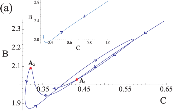
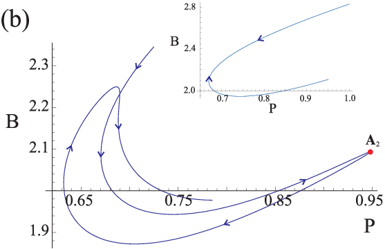
Further information can be found when examining the projections of the whole curve on the -, - and - planes. We show these projections in the case of a Lorentzian spectral distribution having a width ten times larger than that in Fig. 1. Such a choice allows to distinguish more clearly the different curves. All the panels of Fig. 2 show that there is no one-to-one correspondence between any two of the quantities , and . It is interesting to notice that this behavior does not depend on the losses of the cavity, but it remains true also when the environment reduces to a single mode, as seen from the insets of Fig. 2. The absence of one-to-one correspondence between any two of the quantities , and is truly a consequence of the reservoir-mediated interaction between the qubits; in fact, if one examines the dynamics starting from the same initial state, but with the two qubits embedded in independent reservoirs, one-to-one correspondences between these quantities are found. Considering the plot in the - plane, displayed in panel (a), it is possible to see that the system passes through states, for example like those individuated by points and , such that but . This inversion of entanglement ordering has been in general shown for different quantifiers, as between entanglement of formation and either negativity [37] or relative entropy of entanglement [38]. Indeed, there is a region characterized by small values of concurrence () but where the Bell inequality is violated up to values . The - plot of panel (b) gives a justification of this behavior. In fact, as already noticed from Fig. 1 in the -- space, to these small values of concurrence, there correspond high values of purity. In particular, when the maximum of Bell function reaches (point ). This correspondence between small and high values is finally confirmed by the - plot of panel (c). Moreover, it is possible to note that the system crosses the point in the - plane two times (within the time interval we are considering), in correspondence of which two different values of occur, as individuated by the points and in the - plane displayed in panel (c). This means that at the same couple of values , there correspond two different values of (). As a final remark, we note that if one considers the part of plots where the multi-branch behavior of Fig. 1 is retrieved.

For a lossy cavity, the analytic solution for the density matrix element is cumbersome as shown in Ref. [35]. In the following we give these expressions in the simpler case when the common cavity has no losses.
II.3.1 Perfect cavity
For a lossless cavity (single mode reservoir) the density matrix elements of the system can be expressed as function of the population of the super-radiant state and of
| (10) |
and are oscillating functions with different periods (the first being the half of the second one) and their expression is [35]
| (11) |
where is the coupling constant between the qubits and the mode of the cavity. The interaction between the qubits, mediated by the common reservoir, makes the coherence never vanish, as instead happens in the case of independent reservoirs. From the insets of Fig. 2, one sees that there is not a one-to-one correspondence between any two of the quantities , and . Due to the absence of losses in the cavity, the system goes back and forth through the entire curve, meaning that at certain times the qubits recover the pure maximally entangled state of preparation. When dissipation is taken into account and a more complex environment than a single mode is considered this picture becomes more complex and the multi-way behavior in the -- parameter space of Fig. 1 and in the projection planes of Fig. 2 arises.
The analysis above shows that a quite complex interplay occurs among , and . It is known that in general, given two of these quantities, this does not determine the third [25]. However, one may ask if it may happen that some explicit connections among them exist, which can be expressed in a closed form for some class of states.
III -- relation
In this section we seek an equation among , and that may be usefully adopted to quantify their connection in a general context. To this purpose we shall generalize a relation valid only for pure states. It is known that in this latter case, a relation between and holds [16],
| (12) |
In the attempt to generalize this equation to mixed states, we notice that the former equation can be written as with . Therefore, it is rather natural to connect the three quantities , and , for any state, as
| (13) |
where the “remainder” is a quantity expressed in terms of density matrix elements that vanishes for pure states. In particular, four different regions can be distinguished on the basis of and defined in Eqs. (2) and (4):
- •
Region 1: and
(14) - •
Region 2: and
(15) - •
Region 3: and
(16) - •
Region 4: and
(17)
where the symbol means that index must be changed into and viceversa. The introduction of a remainder in Eq. (13) allows us to express the Bell function as a function of concurrence and purity and may explain why states characterized by the same concurrence and purity can have different values of the Bell function. Such a remainder might contain some unknown properties qualifying the state of the system.
Even if in the general case a closed equation between , and does not exist, it may be useful to look for classes of states for which the remainder can be expressed as a function of these same quantities. In the following we show that this occurs in the case of maximally entangled mixed states.
III.1 Application to maximally entangled mixed states
As an example to which to apply the considerations and the formulas above we now consider the case of maximally entangled mixed states (MEMS), defined as those states possessing the maximal amount of entanglement (quantified by tangle or concurrence ) for a given degree of mixedness (quantified by linear entropy or purity ) [18, 19]. MEMS have been generated in laboratory by parametric down conversion [39]; their density matrix depends on the quantifiers chosen for entanglement and mixedness. Typically, tangle is used to quantify entanglement and linear entropy to quantify mixedness. Since the quantities - and - are monotonically related each other, the use of and instead of and does not affect the structure of MEMS density matrix. For these quantifiers the explicit form of MEMS, in the standard computational basis , is given (up to local unitary transformations) by [18]
| (18) |
where the parameter coincides with the concurrence (for any value of the state is entangled) and
| (19) |
According to the parametric regions identified by Eqs. (14)-(17) and the -- relation of Eq. (13), we obtain the following expressions of , , and for various ranges of :
- •
corresponds to region 1 with
(20) - •
corresponds to region 3 with
(21) - •
again corresponds to region 3 with
(22)
Regions 2 and 4 are excluded because for MEMS for any value of . From the last three equations, it follows that Bell inequality violation occurs only for . It is worth to note that in this region of violation the maximum of Bell function assumes the lower bound of violation, , for a given concurrence. This fact can be considered as a further characterization of MEMS [16]. For any value of the remainder results to be a function of only concurrence and vanishes when according to the considerations that follow the -- relation of Eq. (13). We recall that, by varying , the MEMS individuate an upper bound curve in the - plane under which all the two-qubit quantum states are confined [18].
In the following we come back to our dynamical case, showing that choosing properly the initial state, the dynamics of the system flows along this upper bound MEMS curve.
IV Super-radiant state dynamics in -- space and MEMS generation
Here, we investigate the dynamics of the two qubits in the same model of Sec. II.2, in the case they are initially prepared in the one-excitation (super-radiant) Bell state
| (23) |
The trajectory of the representative point of the system in the -- space is shown in Fig. 3.
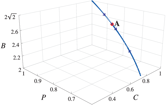
This path is obtained by a dense sampling of triplets of -- values at different times (up to the time ). One sees that the dynamics starts from the pure maximally entangled state (, ), thus maximally violating the CHSH inequality (). Due to the interaction with the environment, , and all decrease and at a certain time the CHSH inequality is not violated anymore. After this time the curve goes below the plane but after a while the memory effects of the non-Markovian environment makes those three quantities simultaneously revive. When the representative point raises above the plane, giving revivals of , it follows again the same curve but runs only a part of it. This is related to the fact that the system is open and environmental noise deteriorates the coherence properties of the state of the system, with a corresponding decrease of the maximum values of and with time. Hence, the dynamics passes through cycles of revivals and collapses until, after a certain time, the CHSH-Bell inequality is not violated anymore.
This behavior can be clearly seen by examining the explicit evolution of the two-qubit density matrix. All the density matrix elements at a given time depend only on the population of the super-radiant state at that time,
| (24) |
Varying the ratio between the spontaneous emission rate and the spectral density width, , two different regimes in the time behavior of can be distinguished. For (weak coupling) there is a Markovian exponential decay controlled by ; for (strong coupling) non-Markovian effects become relevant. In this latter regime the function assumes the form [40]
| (25) |
where . In this strong coupling regime presents damped oscillations while in the weak coupling regime Markovian-like decay occurs (harmonic functions in are replaced with the corresponding hyperbolic ones and with ). In the ideal cavity limit, , becomes a purely oscillating function.
We point out that Eq. (24) corresponds to the density matrix form of MEMS of Eq. (18) (for ) where, after a local unitary transformation on one of the two qubits (changing in and viceversa), plays the role of a time-dependent parameter , whose behavior depends on the values of spectral density parameters. This means that, starting from the super-radiant state, the two-qubit system evolves along the MEMS curve. As a consequence, the physical configuration of two qubits in a lossy common cavity is suitable for a dynamical creation of MEMS (see also other proposals for MEMS generation [41, 42]).
Because of Eq. (25), clearly , and do also depend only on . In particular for the range of values we are in the region 2 (see Sec. III) and CHSH-Bell inequality is never violated; for we are in region 4 where , and assume the form
| (26) |
the CHSH-Bell inequality being violated for . This form of , and implies a closed relation among these three quantities which can be analytically expressed as
| (27) |
where the remainder of Eq. (13) is given by . Eq. (27) corresponds to what obtained in Eq. (22) for MEMS. It is worth to stress that, differently from the general case where no closed relation among , and exists, here we deal with a dynamical case where a closed relation is available. This analytical relation between , and explains why the system draws with time back and forth on the same trajectory in the -- space. Moreover the explicit expressions of Eq. (24) allows to understand why this trajectory remains unaltered when changing the width of the Lorentzian distribution. Indeed, this is a consequence of the fact that each -- point is determined by only one specific value of . In the case of a Lorentzian distribution, exhibits damped oscillations between 0 and 1, so that repeated equal values of give the same -- points and thus in turn the system dynamics draws back and forth the same trajectory in the -- space. On the other hand, the width of the Lorentzian affects the oscillatory behavior of , therefore influencing only the number of times and how high the system can come back on the same curve in the -- space. We emphasize once more that this is true only for this particular initial state.
V Conclusions
In this paper the relation among entanglement, mixedness and nonlocality in a two-qubit system has been investigated. The nontrivial connection among the quantifiers of these properties, namely concurrence , purity and the maximum of Bell function in the state space has been studied in a dynamical context. Two qubits have been assumed to be embedded in a non-Markovian common reservoir at zero temperature. Common reservoir-mediated interaction and memory effects induce, with different intensities, revivals of all the three quantities. The -- “parameter” space has been introduced and exploited for the description of the relations among , and for the two-qubit reduced dynamics.
For an initial two-excitation Bell state, it has been shown that the system draws a multi-branch curve in the -- space. Projection of this curve on two-dimensional spaces clearly shows the absence of one-to-one correspondence between couples of the quantifiers , and [25]. This dynamical feature is maintained even in the limit of perfect cavity suffering no losses. A comparison with the case of independent reservoirs, where this correspondence between couples of the quantifiers occurs, has been made evidencing the role of the common reservoir-mediated interaction between qubits as responsible of the lack of such correspondence.
The search of classes of states where a closed relation among , and holds, has led us to look for general connections among these quantifiers. On the basis of known relations between concurrence and maximum of Bell function in the pure state case, an extended relation between all the three quantifiers for a wide class of mixed states has been given. A remainder, vanishing in the limit of pure state, has been introduced and its explicit form given for four different regions identified by the quantum state under investigation. This term could play a role to explain the complex and not well understood relation among all these quantities. Moreover we have shown that, for the class of maximally entangled mixed states (MEMS), a closed relation among , and exists.
In the final part of the paper we have reconsidered our dynamical model, showing that if the two qubits are initially prepared in the one-excitation Bell state (super-radiant state), differently from the two-excitation case, a one-to-one correspondence between any couple of , and occurs. This results in a single-valued relation represented by a one-branch curve in the -- space which is drawn back and forth by the system. In this case we have a physical configuration in which a closed analytical relation among , and can be written. We have moreover shown that the system evolves maintaining the MEMS density matrix structure. Therefore this physical configuration may be seen as a suitable setup for MEMS generation.
Acknowledgements.
L.M. thanks S. Maniscalco and J. Piilo for useful discussions, and G. Compagno and his group for the kind hospitality at the Università di Palermo. L.M. thanks also M. Ehrnrooth Foundation for financial support.References
- [1] R. Horodecki, P. Horodecki, M. Horodecki, and K. Horodecki, Rev. Mod. Phys. 81, 865 (2009).
- [2] W. K. Wootters, Phys. Rev. Lett. 80, 2245 (1998).
- [3] M. A. Nielsen and I. L. Chuang, Quantum Computation and Quantum Information (Cambridge University Press, 2000).
- [4] J. S. Bell, Physics 1, 195 (1964).
- [5] J. F. Clauser, M. A. Horne, A. Shimony, and R. A. Holt, Phys. Rev. Lett. 23, 880 (1969).
- [6] M. Horodecki, P. Horodecki, and R. Horodecki, Phys. Lett. A 200, 340 (1995).
- [7] A. Acin, N. Gisin, and L. Masanes, Phys. Rev. Lett. 97, 120405 (2006a).
- [8] N. Gisin and R. Thew, Nature Photon. 1, 165 (2007).
- [9] S. Popescu, Phys. Rev. Lett. 72, 797 (1994).
- [10] L. Masanes, Y.-C. Liang, and A. C. Doherty, Phys. Rev. Lett. 100, 090403 (2008).
- [11] M. Forster, S. Winkler, and S. Wolf, Phys. Rev. Lett. 102, 120401 (2009).
- [12] N. Gisin, Phys. Lett. A 154, 201 (1991).
- [13] R. F. Werner, Phys. Rev. A 40, 4277 (1989).
- [14] J. Barrett, Phys. Rev. A 65, 042302 (2002).
- [15] A. Acin, N. Gisin, and B. Toner, Phys. Rev. A 73, 062105 (2006b).
- [16] F. Verstraete and M. M. Wolf, Phys. Rev. Lett. 89, 170401 (2002).
- [17] A. Miranowicz and A. Grudka, J. Opt. B: Quantum Semiclass. Optics 6, 542 (2004).
- [18] W. J. Munro, D. F. V. James, A. G. White, and P. G. Kwiat, Phys. Rev. A 64, 030302 (2001a).
- [19] T.-C. Wei, K. Nemoto, P. M. Goldbart, P. G. Kwiat, W. J. Munro, and F. Verstraete, Phys. Rev. A 67, 022110 (2003).
- [20] M. Ziman and V. Bužek, Phys. Rev. A 72, 052325 (2005).
- [21] E. S. Cardoso and V. Buzek, Phys. Rev. A 72, 042320 (2005).
- [22] W. J. Munro, K. Nemoto, and A. G. White, J. Mod. Opt. 48, 1239 (2001b).
- [23] S. Ghosh, G. Kar, A. Sen(De), and U. Sen, Phys. Rev. A 64, 044301 (2001).
- [24] L. Derkacz and L. Jakóbczyk, Phys. Lett. A 328, 26 (2004).
- [25] L. Derkacz and L. Jakóbczyk, Phys. Rev. A 72, 042321 (2005).
- [26] B. Bellomo, R. Lo Franco, and G. Compagno, Phys. Rev. Lett. 99, 160502 (2007).
- [27] B. Bellomo, R. Lo Franco, S. Maniscalco, and G. Compagno, Phys. Rev. A 78, 060302(R) (2008a).
- [28] Z. Ficek and R. Tanaś, Phys. Rev. A 74, 024304 (2006).
- [29] B. Bellomo, R. Lo Franco, and G. Compagno, Phys. Rev. A 77, 032342 (2008b).
- [30] E. Hagley et al., Phys. Rev. Lett. 79, 1 (1997).
- [31] S. Bose, I. Fuentes-Guridi, P. L. Knight, and V. Vedral, Phys. Rev. Lett. 87, 050401 (2001).
- [32] P. G. Kwiat, S. Barraza-Lopez, A. Stefanov, and N. Gisin, Nature 409, 1014 (2001).
- [33] J. S. Pratt, Phys. Rev. Lett. 93, 237205 (2004).
- [34] J. Wang, H. Batelaan, J. Podany, and A. F. Starace, J. Phys. B 39, 4343 (2006).
- [35] L. Mazzola, S. Maniscalco, J. Piilo, and K.-A. Suominen (2009a), eprint: quant-ph/0904.2857.
- [36] L. Mazzola, S. Maniscalco, J. Piilo, K.-A. Suominen, and B. M. Garraway, Phys. Rev. A 79, 042302 (2009b).
- [37] J. Eisert and M. B. Plenio, J. Mod. Phys. 46, 145 (1999).
- [38] A. Miranowicz, S. Ishizaka, B. Horst, and A. Grudka, Phys. Rev. A 78, 052308 (2008).
- [39] N. A. Peters, J. B. Altepeter, D. Branning, E. R. Jeffrey, T.-C. Wei, and P. G. Kwiat, Phys. Rev. Lett. 92, 133601 (2004).
- [40] S. Maniscalco, F. Francica, R. L. Zaffino, N. Lo Gullo, and F. Plastina, Phys. Rev. Lett. 100, 090503 (2008).
- [41] S.-B. Li, Phys. Rev. A 75, 054304 (2007).
- [42] S. Campbell and M. Paternostro, Phys. Rev. A 79, 032314 (2009).