Concentration of measure for quantum states with a fixed expectation value
Abstract
Given some observable on a finite-dimensional quantum system, we investigate the typical properties of random state vectors that have a fixed expectation value with respect to . Under some conditions on the spectrum, we prove that this manifold of quantum states shows a concentration of measure phenomenon: any continuous function on this set is almost everywhere close to its mean. We also give a method to estimate the corresponding expectation values analytically, and we prove a formula for the typical reduced density matrix in the case that is a sum of local observables. We discuss the implications of our results as new proof tools in quantum information theory and to study phenomena in quantum statistical mechanics. As a by-product, we derive a method to sample the resulting distribution numerically, which generalizes the well-known Gaussian method to draw random states from the sphere.
I Introduction
The term concentration of measure phenomenon refers to the observation that in many high-dimensional spaces “continuous functions are almost everywhere close to their mean”. A well-known illustration is the fact that on a high-dimensional sphere “most points lie close to the equator”. In other words, the values of the coordinate functions concentrate about , their mean. On the sphere, the effect exists not only for coordinate functions, but for any Lipschitz-continuous function. The result—known as Lévy’s Lemma—has surprisingly many applications in both mathematics and physics (see below).
Our main contribution is a “Lévy’s Lemma”-type concentration of measure theorem for the set of quantum states with fixed expectation value.
More concretely, suppose that we are given any observable with eigenvalues on . In the following, we will often call a “Hamiltonian” and the “energy levels”, but this is not the only possible physical interpretation. We fix some arbitrary value , and we are interested in the set of pure quantum states with fixed expectation value , i.e.,
Our main Theorem 1 shows that, subject to conditions on the spectrum of , any continuous function on concentrates about its mean.
The motivation for the approach taken here is two-fold.
I.1 Motivation 1: The probabilistic method
Beyond being a geometric curiosity, the concentration of measure effect is a crucial ingredient to an extremely versatile proof technique: the probabilistic method [1]. Recall the basic idea. Assume, by way of example, one wants to ascertain the existence of a state vector on qubits, such that is “highly entangled” with respect to any bipartition of the systems into two sets. The problem seems daunting: There are exponentially many ways of dividing the composite system into two parts. For any bipartition, we need to make a statement about the entropy of the eigenvalue distribution of the reduced density matrix – a highly non-trivial function. Lastly, in any natural parametrization of the set of state vectors, a change of any of the parameters will affect the vast majority of the constraints simultaneously.
Given these difficulties, it is an amazing fact that the probabilistic method reduces the problem above to a simple lemma with a schematic proof (detailed, e.g., in Ref. [3, 2]). Neither the non-trivial nature of the entropy function, nor the details of the tensor product space from which the vectors are drawn enters the proof. Only extremely coarse information – the Lipschitz constant of the entropy and the concentration properties of the unit sphere – are needed.
Consequently, proofs based on concentration properties are now common specifically in quantum information theory. Examples include the investigation of “generic entanglement” [3], random coding arguments to assess optimum rates in quantum communication protocols, state merging [5], the celebrated counterexample to the additivity conjecture in quantum information theory [6], or the resource character of quantum states for measurement-based computing [7, 8].
The tremendous reduction of complexity afforded by the probabilistic method motivates our desire to prove measure concentration for other naturally occurring spaces, besides the sphere. For the set of “states under a constraint”, Theorem 1 achieves that goal and opens up the possibility of applying randomized arguments in this setting.
I.2 Motivation 2: Statistical mechanics
The second motivation draws from notions of quantum statistical mechanics [13, 9, 10, 11, 12, 14, 15, 16, 17, 18]. The predictions of statistical mechanics are based on ensemble averages, yet in practice prove to apply already to single instances of thermodynamical systems. This phenomenon needs to be explained. It becomes at least plausible if there is a measure concentration effect on the ensemble under consideration. Concentration implies that any observable will give values close to the ensemble mean for almost every state in the ensemble. This will in particular happen at almost every point on a sufficiently generic trajectory through the ensemble. Thus there may be an “apparent relaxation” [10, 11, 15, 16, 17, 18] even in systems not in a global equilibrium state.
Recently, several authors realized that it is particularly simple to state a precise quantitative version of this intuition for ensembles consisting of random vectors drawn from some subspace [10, 18]. However, in the context of statistical mechanics, it may be more natural to consider sets of states with prescribed energy expectation value, rather than elements of some linear subspace. Indeed, such “mean energy ensembles” have been studied before [19, 20, 21, 22]. Thus, it is natural to ask whether the concentration results for linear spaces translate to mean energy ensembles.
We present both positive and negative results on this problem. Since the mean energy ensemble and its properties depend on the spectrum of the chosen observable , so does the degree of measure concentration. For many spectra typically encountered in large many-body systems, our main theorem yields trivial bounds. As explained in Section III, this is partly a consequence of the fact that “Lévy’s Lemma-type” exponential concentration simply does not exist for such systems. However, for families of Hamiltonians with, for example, constant spectral radius, we do get meaningful concentration inequalities. Therefore, the methods presented in this paper are expected to have a range of applicability complementary to other approaches.
The question whether weakened concentration properties can be proven for more general many-body systems under energy constraints remains an interesting problem (see Section III).
II Main Results and Overview
As stated above, we will analyze the set
for some observable and expectation value . The set of all pure quantum states is a complex sphere in ; equivalently, we can view it as the unit sphere in . The obvious geometric volume measure on corresponds to the unitarily invariant measure on the pure quantum states [3]. As we will see below, the set is a submanifold of the sphere (and thus of ); hence it carries a natural volume measure as well, namely the “Hausdorff measure” [23] that it inherits from the surrounding Euclidean space . Normalizing it, we get a natural probability measure on .
Our first main theorem can be understood as an analog of Lévy’s Lemma [24] for the manifold . It says that the measure on is strongly concentrated, in the sense that the values of Lipschitz-continuous functions are very close to their mean on almost all points of . In some sense, almost all quantum states with fixed expectation value behave “typically”. To understand the theorem, note that is invariant with respect to energy shifts of the form , , such that the new eigenvalues are . We then have , i.e., the manifold of states does not change (only its description does). We call a function -Lipschitz if it satisfies , where denotes the Euclidean norm in .
Theorem 1 (Concentration of measure).
Let be any observable on , with eigenvalues , , , and arithmetic mean . Let be any value which is not too close to the arithmetic mean, i.e.,
Suppose we draw a normalized state vector randomly under the constraint , i.e., is a random state according to the natural distribution described above. Then, if is any -Lipschitz function, we have
| (1) |
where is the median of on , and the constants , and can be determined in the following way:
- •
Shift the energies by some offset (as described above) such that and
(2) with , where denotes the harmonic mean energy. The offset may be chosen arbitrarily subject only to the constraint that the constant below is positive.
- •
Compute and
The theorem involves an energy offset , shifting all energy levels to . The idea is to choose this shift such that , i.e. such that the energy in question becomes close to the harmonic mean energy (we show in Lemma 20 below that this is always possible). Specifically, the theorem demands that becomes a bit larger than , resulting in a constant defined in eq. (2). The theorem does not specify uniquely – there is some freedom for optimizing over the different possible choices of . However, there is the constraint that , which prevents us from choosing too small values of (indeed, is equivalent to ). On the other hand, should not be too large, because it appears in the exponent in eq. (1).
To apply the theorem, it is often useful to know the value of the median . Our second main theorem gives an approximation of in the limit :
Theorem 2 (Estimation of the median ).
With the notation from Theorem 1, let be the full ellipsoid
and let be any -Lipschitz function. Then, the median of on the energy manifold satisfies
where .
We proceed by discussing a simple example. Suppose we have a bipartite Hilbert space with dimensions and large, but arbitrary , and the Hamiltonian
| (3) |
We fix the arbitrary energy value , and draw a state randomly under the constraint , which is . What does Theorem 1 tell us about concentration of measure for this manifold of quantum states? To have all positive eigenvalues, our offset must be , and the shifted harmonic mean energy becomes
The offset (equivalently, the constant ) is not specified uniquely by Theorem 1; we try to find a good choice by fixing independently of . After some trial-and-error, turns out to be a good choice (other values work as well, but not ). The next task is to estimate the shift which results from our choice of ; it is determined by the equation
where . It is difficult to solve this equation directly, but it is easy to see that a solution close to exists for large . This fact helps to gain a rough estimate of which is sufficient to prove strong concentration of measure: denote the difference of the left- and right-hand side by , then for all . Since is decreasing, we get for all , hence . The constant
is increasing in , hence , and similarly . On the other hand, since for all , we have . Hence we have to consider the expression only in the relevant interval , where it is decreasing and thus upper-bounded by . Consequently, is positive and satisfies . Substituting these expressions into Theorem 1, we get the following result:
Example 3.
Drawing random pure state vectors under the constraint , where is the observable defined in eq. (3), we get the concentration of measure result
for every -Lipschitz function and all .
It is clear that the amount of measure concentration that we get from Theorem 1 depends sensitively on the spectrum of the Hamiltonian . In particular, not all natural Hamiltonians yield a non-trivial concentration result. For example, in Section III, we show that for a sequence of non-interacting spins, Theorem 1 does not give a useful concentration result in the sense that the corresponding concentration constant in (1) will be very close to zero. However, we will also prove that this is not a failure of our method, but reflects the fact that there simply is no concentration in that case, at least no concentration which is exponential in the dimension.
In the “thermodynamic limit” of large dimensions , the condition on the energy in Theorem 1 becomes . From a statistical physics point of view, is the ground state energy of “temperature zero”, while corresponds to the “infinite temperature” energy. Hence, the condition on can be interpreted as a “finite temperature” condition. However, this condition is no restriction: if one is interested in concentration of measure for , then the simple substitution and will make Theorem 1 applicable in this case as well.
In the situation of Example 3 above, with Hamiltonian (3) on the bipartite Hilbert space with fixed and large , we may ask what the reduced density matrix typically looks like. It is well-known [3] that for quantum states without constraints, the reduced density matrix is typically close to the maximally mixed state. To estimate the typical reduced state in our case, we may consider the Lipschitz-continuous functions , that is, the matrix elements of the reduced state. Theorem 2 gives a way to estimate these matrix elements by integration over some ellipsoid.
Instead of doing this calculation directly, we give a general theorem below which gives the typical reduced density matrix in the more general case that the global Hamiltonian can be written
i.e., if it describes two systems without interaction. The Hamiltonian (3) corresponds to the special case . In this case, we get:
Example 4.
Random state vectors under the constraint , where is the observable defined in (3), typically have a reduced density matrix close to
More in detail, we have for all and
This example is a special case of our third main theorem:
Theorem 5 (Typical reduced density matrix).
Let be an observable in the Hilbert space of dimension with . Denote the eigenvalues of and by and , and the eigenvalues of by respectively. Suppose that the assumptions of Theorem 1 hold, and adopt the notation from there, in particular, with the energy offset specified there. Then, the reduced density matrix of random pure state vectors under the constraint satisfies
for all , where the “canonical” matrix is given by
and the constant equals
where .
The “canonical” matrix given above does not immediately have a useful physical interpretation.
In particular, it is not in general proportional to , i.e., it is not necessarily
the Gibbs state corresponding to as one might have expected based on intuition
from statistical mechanics (we discuss this point in more detail in Section III below).
Note also that is not exactly normalized, but it is close to being normalized (i.e.,
in large dimensions , which follows from ).
To illustrate the use of Theorem 5, we give a proof of Example 4. We use the notation and intermediate results from the proof of Example 3. The energy shift depends on the dimension , i.e., , and we have . More in detail, if we use Mathematica to compute the Taylor expansion of at , we find the inequality
| (4) |
for all . The typical reduced density matrix that Theorem 5 supplies depends on . It is
which tends to the matrix from the statement of Example 4 as . We can use eq. (4) to bound the difference between and . Using that is decreasing in , while and are increasing, a standard calculation yields
| (5) |
for all . Similar calculations can be used to bound the constant from above: for all . Thus, according to Theorem 5, it holds
for all . The estimate (5) together with proves the claim in Example 4. ∎
An interesting aspect of Theorem 5 is that the typical reduced density matrix does not maximize the entropy locally (if so, it would be the Gibbs state corresponding to ). This is expected to have applications in quantum information theory in situations where random bipartite states with non-maximal entanglement are considered. It will be shown in Section IV below that the reduced density matrices maximize a different functional instead which is related to the determinant.
III Implications for Statistical Mechanics
Recently, the concentration of measure phenomenon has attracted a considerable amount of attention in the context of quantum statistical mechanics. Consider some ensemble of quantum states, such as the set of all pure quantum states in a certain subspace of the global Hilbert space. The subspace might be given, for example, by the span of all eigenvectors corresponding to an energy in some small interval with respect to a given Hamiltonian .
Suppose we are given a single, particular, random state vector from this subspace. What properties will this pure state have? At first one might be tempted to think that there is very little knowledge available on the properties of the state, and that most properties should turn out to be random. However, the concentration of measure phenomenon shows that this is not the case – almost all the possible state vectors will have many properties in common.
Several authors [13, 9, 10, 11, 12] have recently argued that this property of measure concentration may help to better understand certain foundational issues of statistical mechanics. Conceptually, statistical mechanics aims to predict outcomes of measurements on systems even in the case that we have only very limited knowledge about the system (say, we only know a few macroscopic variables). Ensemble averages are employed to make predictions, and the predictions agree very well with experiment even in single instances of the system. Concentration of measure is then viewed as a possible theoretical explanation of some aspects of this phenomenon.
As a paradigmatic example, Ref. [10] considers the situation of a bipartite Hilbert space , consisting of system and environment . Then the setting is investigated where the set of physically accessible quantum states is a subspace (for example, a spectral windows subspace as explained above). If we are given an unknown random global quantum state vector , then what does the state typically look like for the system alone? In this case, the postulate of equal apriori probabilities from statistical physics suggests to use the maximally mixed state on , that is , as an ensemble description. Then, taking the partial trace over the environment will yield a state which may be used by observers in to predict measurement outcomes.
According to Ref. [10], concentration of measure in the subspace proves that almost all quantum state vectors have the property that the corresponding reduced state is very close to . That is, with overwhelming probability. It is then argued in Ref. [10] that this result explains why using the ensemble average is in good agreement with experiment even in the case of a single instance of the physical system.
While Ref. [10] considers a very general situation that does not allow for specifying directly what the “typical” state looks like, Ref. [9] make additional assumptions that allow to specify in more detail. That is, if the Hamiltonian is
(that is, there is no or negligible interaction between system and environment), if the restriction is given by a spectral energy window, and if the bath’s spectral density scales exponentially, then for some suitable . That is, under these standard assumptions from statistical mechanics, Ref. [9] argues that the typical reduced state is a Gibbs state.
These results raise an immediate question: what happens if the restriction is not given by a subspace? In statistical mechanics, one often considers the situation that an observer “knows the total energy of the system”, but does not know the exact microscopic state. In all the papers previously mentioned, the intuitive notion of “knowing the energy” has been translated to the technical statement of “knowing with certainty that the quantum state is supported in a spectral subspace”. Obviously, there is at least one natural alternative: knowing the energy might also be read as “knowing the energy expectation value of ”.
In fact, this possibility has been proposed by several authors [19, 20, 21] as a possible alternative definition of the “quantum microcanonical ensemble” (we call it “mean energy ensemble”). The results in this paper give some information on the applicability of the mean energy ensemble in statistical mechanics:
- 1.
As a positive result, we know from Theorem 1 that the concentration of measure phenomenon occurs for the mean energy ensemble as well, if that theorem is applicable to the particular Hamiltonian and energy value that is considered. In this case, many interesting results from Refs. [13, 9, 10, 11, 12] carry over to the mean energy ensemble.
- 2.
On the other hand, the ensemble does not seem to reproduce well-known properties of statistical mechanics, such as the occurrence of the Gibbs state (cf. Theorem 5). Hence it seems to describe rather exotic physical situations.
There is an intuitive reason why the mean energy ensemble behaves exotically: calculations involving Theorem 2 suggest that the -th energy level typically has an occupation proportional to , where is the corresponding shifted energy value (cf. Theorem 1); this is also visible in the form of the typical reduced density matrix in Theorem 5. In particular, typical state vectors “spread out” a lot on the small energy levels. This produces a “Schrödinger cat state” which is in a coherent superposition of many different energy states. Such states are not normally observed in statistical physics.
However, point 2. does not completely rule out the mean energy ensemble as a description of actual physics, due to the following fact:
- 3.
Our result is tailor-made for systems with the property that the corresponding mean energy ensemble concentrates exponentially in the dimension , similarly as in Lévy’s Lemma (corresponding to inequality (6) below with ). However, many natural many-body systems do not have such a concentration property, which is why Theorem 1, 2 and 5 do not apply in those cases.
As an example, we will now show that the mean energy ensemble does not concentrate exponentially in the case of non-interacting spins. Let the energy levels of each spin be and . The total Hilbert space has dimension . If is an integer between and , then the energy level is -fold degenerate. Moreover, suppose that we are interested in the energy value , where . To see if Theorem 1 is applicable, we determine a rough estimate of the energy shift that has to be employed such that . We thus have to find such that
this is only possible if the -term gives a significant contribution. The conclusion is that must be very small, that is, of the order (and this conclusion is confirmed by more elaborate large deviations arguments similar to those discussed below). But then, the constant in the exponent in (1) is approximately
such that Theorem 1 does not give any measure concentration at all.
It turns out, however, that this result is not a failure of our method, but reflects the fact that there simply is no concentration of measure which is exponential in the dimension in this case. The precise statement below makes use of the binary entropy function
defined for (c.f. [25]).
Example 6 (Non-interacting spins: no exp. concentration).
Suppose we have non-interacting spins as explained above, and fix the energy value with . Consider a hypothetical concentration of measure inequality
| (6) |
for all -Lipschitz functions . Here, denotes either the mean or the median of , is the dimension of the system and a fixed constant. If such an inequality is to hold, then necessarily
| (7) |
for any . In particular, the optimal exponent in (7) is strictly smaller than one if and goes to zero as .
Proof.
Let be such that . Let
Normalization gives from which we get
| (8) | |||||
We can also bound using inequality (6). To this end, consider the -Lipschitz function , that is, the real part of the -th component of in the Hamiltonian’s eigenbasis. Due to the invariance of the energy manifold with respect to reflections , both expectation value and median of this function equal zero. If hypothesis (6) is true, then it follows by squaring that
and thus
| (9) | |||||
having used integration by parts. An analogous inequality obviously holds for the imaginary part . From basic information theory (e.g., Chapter 11 in Ref. [25]), we borrow the fact that the number of terms in the definition of is upper-bounded by
| (10) |
for every . ∎
It is highly plausible that similar results hold for the mean energy ensemble of many other many-body systems: the best possible rate of concentration (such as the right-hand side in (6)) is not , but at most with energy-dependent exponent . Deciding whether this upper bound can be achieved remains an interesting open problem. Indeed, we end the present section by sketching a possible route for tackling this question.
The proof of Example 6 uses the coordinate functions as an example for continuous functions without strong concentration properties. We conjecture that this is already the worst case, i.e. that no function with Lipschitz-constant equal to one “concentrates less” than the “most-spread out” of the coordinate functions.
A strongly simplified version of this conjecture is easily made precise. We restrict attention to real spaces and linear functions
of the state vectors. Here, the ’s are the coefficients of in the eigenbasis of the Hamiltonian and the ’s are arbitrary coefficients subject to the normalization constraint . The latter constraint ensures that the Lipschitz constant of the linear funtion is one. If the vectors are drawn from an energy ensemble , we have the elementary estimate
having made use of the fact that is invariant under the transformation which takes for some while leaving the other coordinates fixed.
Upper bounds on the variance of a random variable are sufficient to establish simple concentration estimates (by means of Chebychev’s inequality). From that point of view, we have proven that coordinate functions show the least concentration among all linear functions, according to methods based on second moments alone. Generalizing this observation to more general functions and higher moments would allow us to restrict attention to the eigenbasis of the Hamiltonian, thus “taking the non-commutativity out of the problem”. Conceivably, this would constitute a relatively tractable path to a more complete understanding of concentration in typical many-body systems.
IV Invitation: a simple Hamiltonian
As a preparation for the proof in the next section, we give a particularly simple example of a Hamiltonian which admits a more direct proof of concentration of measure; in the meantime, we will also see that the “harmonic mean energy” from Theorem 1 appears naturally. Consider a bipartite quantum system on a Hilbert space , with dimensions and . We may assume without restriction that . We are interested in the manifold of state vectors with average energy , where is some Hamiltonian on . What happens if we draw a state from that submanifold at random? Instead of studying this question in full generality (which we will do in Section V), we start with the simple example
where is an observable on alone. This is a special case of a more general bipartite Hamiltonian without interaction as studied in Theorem 5. A nice consequence is that
that is, the constraint depends on the reduced density matrix alone.
The unitarily invariant measure on the pure quantum states on the global Hilbert space induces in a natural way a measure on the density matrices in : if is some measurable subset of the density matrices, then
Formally, the measure is the pushforward measure [26] of the unitarily invariant measure on the pure states of with respect to the map ; that is, .
Due to the simple form of the Hamiltonian , we may calculate probabilities with respect to . The probability density distribution corresponding to is invariant with respect to unitaries on , but it depends on the eigenvalues of the reduced density matrix . The relation is [2, 27]:
| (11) |
where is the normalization constant and .
We will now study the simplest case , where
and we may assume without loss of generality that . We fix some arbitrary energy value between and . Since the average energy is the energy of an “infinite temperature” Gibbs state, we additionally assume that , which is no restriction, but saves us some distinction of cases. Thus, .
The state space is now the Bloch ball; that is, the unit ball in . The distribution has been calculated for the case already by Hall [28]. In ordinary spherical coordinates, it can be written
where , and is some normalization constant. It can be derived from eq. (11) by using that points in the Bloch ball correspond to density matrices with eigenvalues and . If , this measure becomes the usual Euclidean measure in the Bloch ball, corresponding to the Hilbert-Schmidt measure [27]. In general,
We write for .
It is easy to see (and we will show this below) that the subset of mixed states in the Bloch ball with is the intersection of a plane with the Bloch ball; that is, a disc . To determine probabilities, we need to compute the area of two-dimensional subsets . In light of the density introduced above, it is tempting to use the term as the measure of . The normalized version is a probability measure:
| (12) |
It turns out that this measure agrees with the normalized geometric volume measure that we use elsewhere in this paper (for example in Theorem 1). We discuss this fact in detail below after the proof of Proposition 7. Using this identity and deferring its justification to below, we get a concentration of measure result:
Proposition 7.
The reduced density matrix concentrates exponentially on the canonical state
that is,
for all .
Proof.
It follows from the condition that must have diagonal elements
where . By Schur’s Theorem [29], the eigenvalues and of must majorize the diagonal elements, that is, , hence . Thus, among all states satisfying the energy condition, the canonical state is the “most mixed” one, in the sense that its radius in the Bloch ball is the smallest possible.
Geometrically, this has the following interpretation. Translating the condition to the Bloch ball representation, that is, representing density matrices by vectors , we get
This defines a plane with
in ; the intersection of that plane with the Bloch ball gives the set of density matrices that fulfill the energy condition. This set is a disc , with the vector representation of at its center. Since the trace distance on the density matrices corresponds to the Euclidean distance in the Bloch ball, the set of states satisfying the energy condition with corresponds to an annulus in with inner radius ; we denote this annulus by . Hence
By elementary integration, we get
Since , this yields
Substituting
proves the claim. ∎
In this paper, the measure that we are interested in is the Hausdorff volume measure on the energy manifold . To compute the correct probabilities when restricting to the Bloch ball by partial trace, we need to invoke the pushforward of with respect to . So is the probability measure that we have defined above in eq. (12) equal to this pushforward measure, i.e., does
hold? Fortunately the answer is “yes”, but this is not directly obvious. First we observe that may be interpreted as an “energy shell measure” in the following sense. The submanifold measure from eq. (12) can be given by a limit, in a spirit similar to the definition of the “Minkowski content” (cf. Ref. [23]): For , denote by the set of matrices that are -close to , and have an energy expectation value of . This is half of the -neighborhood of . Then, up to a normalization constant,
But is a “slice” of the Bloch ball in between two parallel planes. The set consists of those matrices determined by the inequality , where is some energy difference corresponding to . In particular,
This is an energy shell. Hence it is basically the uniform distribution on this energy shell on the pure states which, by taking the partial trace and the limit , generates our probability measure .
In the general case of arbitrarily many different energy levels , this energy shell has different “widths” at different points ; in the limit , this width is proportional to , where denotes the projection onto the sphere’s tangent space at . Hence the corresponding “energy shell measure” does not in general equal the geometric (Hausdorff) measure used elsewhere in this paper, which arises from an analogous limit procedure, but starting with the uniform distribution in an -neighborhood of .
However, here we are in a very special situation: we only have two different energy levels and which are highly degenerate. In this case, it turns out that is constant along . To simplify the argument, we double the dimensions and work in real space ; the case applies to Proposition 7 above.
Lemma 8.
Consider the real energy manifold
in the special case that there are only two different energy levels, i.e. there exist such that , and . Furthermore, assume that . Let denote the projection onto the tangent space of the unit sphere, and let . Then, is constant on .
Proof.
Direct calculation yields
where . Since
equals on all of , it follows that is constant on . But then,
is also constant on all of . ∎
Hence, in our case of only two different energy levels, the energy shell has constant width everywhere, such that the measure defined in eq. (12) indeed agrees with the geometric measure that we use elsewhere in the paper.
Proposition 7 shows that a typical reduced density matrix is close to ; that is, it is diagonal in -basis, and it can be written with and some appropriate “inverse temperature” . Hence it is a Gibbs state.
This result suggests that the local state always concentrates on a Gibbs state when , also in the more general case . But this guess is false, as we have already shown in Theorem 5 and Example 4 – the local density matrix always commutes with , but it is not in general the corresponding Gibbs state.
In light of the calculation above, it is now easy to give an intuitive explanation for this fact. In analogy to the previous proposition for , we expect that the distribution of eigenvalues as given in eq. (11) will dominate the concentration of measure to some local “canonical” state. It also seems reasonable to assume (and can be verified numerically) that the -terms do not contribute much for large , and that the other terms exponential in dominate. But these terms are
and so we conclude that the reduced density matrix should concentrate on the one which maximized the previous expression. This suggests the following conjecture:
Conjecture 9.
Suppose that is a Hamiltonian on a bipartite Hilbert space with fixed and varying . Then typical quantum states with fixed mean energy have the property that concentrates exponentially on the determinant maximizer
given the maximizer is unique.
We will now see that the prediction of this conjecture is consistent with Theorem 5. To this end, we now compute the determinant maximizer explicitly. First of all, it is easy to see that must be diagonal if written in the basis of , i.e., : Suppose is any density matrix with , and let denote the diagonal elements. Then , where denotes the eigenvalues of . Now if is the matrix with diagonal elements and other entries zero, then is still true, but by the Hadamard determinant theorem [29]
Hence the maximizer is diagonal; it remains to determine its diagonal elements . We have to maximize subject to the constraints and . It turns out to be difficult to do that directly, so we drop the normalization condition for the moment and solve the resulting equation
where is the Lagrange multiplier. This gives , and . Since this distribution is not automatically normalized, we can use the freedom to shift the energy levels by some offset , i.e., , . The resulting distribution is normalized, i.e., , if and only if
that is, if the offset is shifted such that the new energy value equals the harmonic mean energy . We have thus reproduced the canonical density matrix of Theorem 5. Moreover, the calculation above shows that the occurrence of the harmonic mean energy is very natural and not a technical artifact of our proof. (In Section VI, we give a method for numerical sampling of the energy manifold, and there, the harmonic mean energy will appear in a natural way as well.)
V Proof of main theorem
Before proving the main theorems, we fix some notation that will be useful for the proof. Following the lines of Gromov [26], we define a metric measure space to be a separable complete metric space with a finite Borel measure , i.e., . (In fact, one could more generally consider Polish spaces with a –finite Borel measure, as described by Gromov.) In this paper, we will only consider the two cases that is the energy manifold , or a full ellipsoid , both equipped with the obvious geometric measure and the metric that is induced by the surrounding Euclidean space (for more details, see Section V).
We denote the -sphere by , and the -ball is denoted , i.e.,
The symbol is used for the topological boundary, for example, .
We denote the -dimensional (Hausdorff) volume measure on -dimensional submanifolds by . In case that , we write for the normalized measure on , i.e.,
for Borel subsets . Sometimes we consider subsets that are not actually submanifolds, but are turned into submanifolds in an obvious way. For example, the Ball is itself a metric measure space, but not a submanifold, since it is not open. However, its interior is a submanifold of , and
while . Expectation values with respect to are denoted .
Given some Hamiltonian on , we would like to prove concentration of measure for the “mean energy ensemble”
To relate our discussion to real-valued geometry, we work instead in with . That is, doubling all energy eigenvalues of to get the energy levels , and slightly abusing notation, we can write
Geometrically, is the intersection of the unit sphere with an ellipsoid (given by the energy condition). The action of shifting all energies by some offset (as postulated in Theorem 1) alters the ellipsoid, but not the ellipsoid’s intersection with the sphere; it leaves invariant. It is interesting to note that the corresponding full ellipsoid’s volume turns out to be minimal exactly if the energy shift is tuned such that , i.e., for the harmonic mean energy shift close to the one which is postulated in Theorem 1.
We would like to prove measure concentration for the algebraic variety in ordinary Euclidean space. Introducing a function via
we can write
If is any energy value with and for all , then the differential has full rank on all of , such that is a proper submanifold of of codimension .
If for some (but and ), the eigenvectors corresponding to this energy value are singular points of . Still, removing those eigenvectors from , we get a valid submanifold of of codimension . Since and agree up to a set of measure zero, we will drop the tilde in the following, and simply write for the manifold with eigenvectors removed. If we treat as a metric measure space, we include the eigenvectors in its definition to have a complete metric space.
As a submanifold of , the sets carry a natural geometric volume measure. Since every is a compact submanifold, it makes sense to talk about the normalized measure on , and to ask whether this measure exhibits a concentration of measure phenomenon. Our main proof strategy to answer this question in the positive is due to Gromov [26]. To explain this strategy, we introduce the notion of a “typical submanifold”. Suppose that is a metric measure space, and is a subset (say, a submanifold) which is itself a metric measure space. Then we say that “ is typical in ” if has small codimension, and if a small neighborhood of covers almost all of . That is, already for small .
For example, given an -dimensional sphere , any equator (which is itself an -dimensional sphere) is typical in ; this is just Lévy’s Lemma. On the other hand, a polar cap with angle is only typical in if .
Gromov’s idea can now be explained as follows:
-
If is a metric measure space that shows concentration of measure, and if is a typical submanifold of , then shows measure concentration as well: it “inherits” concentration of measure from .
The intuitive reason why this idea works is as follows. Consider the behavior of Lipschitz-continuous functions on . By continuity, those functions do not change much if we turn to an -neighborhood of ; but then, since is assumed to be typical in , we already obtain almost all of , and so the behavior of the functions on will be similar to that on – in particular, expectation values will be similar, and the concentration of measure phenomenon will occur in if it occurs in . However, Gromov seems to explore this idea in his book only for the case that is a sphere.
In our case, we have to find a submanifold which is itself subject to the concentration of measure phenomenon, such that holds and such that is typical in . A first obvious guess is to use the sphere itself; clearly, is a subset of the sphere , and we have concentration of measure on the sphere by Lévy’s Lemma. However, can only be typical in if the energy is close to the “typical” value , which turns out to be the mean value . Since we definitely want to consider different energies far away form the mean energy, is not a useful choice. Instead, it will turn out that we can choose to be a full ellipsoid with appropriate equatorial radii (in fact, will be the slightly enlarged full energy ellipsoid for an appropriate energy shift).
Our main tool from integral geometry is the Crofton formula [30, 31]. It expresses the volume of a submanifold of in terms of the average volume of intersection of that manifold with random hyperplanes.
Lemma 10 (The Crofton formula [30]).
Let be a -dimensional submanifold of . Consider the invariant measure on the planes of dimension in . If ,
where , and denotes the surface area of the -sphere.
Note that the Crofton formula is formulated in Ref. [30, (14.69)] only for the case that is a compact submanifold, but the proof remains valid also in the case that is not compact. This observation is also expressed in Ref. [31].
For the details of the definition of the invariant measure , see Ref. [30]. In short, the Lie group of all motions (translations and rotations) in possesses the closed subgroup of motions leaving a fixed -dimensional plane invariant. Then, there is a one-to-one correspondence between the set of -planes in and the homogeneous space . Since both and are unimodular, possesses an invariant density which can then be interpreted as a density on the -planes in .
Note that this measure is defined only up to some multiplicative constant – different authors use different normalizations (cf. Ref. [32]), which gives different constants instead of in Lemma 10. However, for fixed and , we always have
and it is only those ratios that are relevant for the calculations. If , then equals the number of points in the set . A useful possible expression for the constants is [32]
The Crofton formula will be useful in the following lemma, which gives a lower bound on the measure of -neighborhoods of subsets of . Given any subset (say, any curve), directly estimating seems difficult – if the curve intersects itself many times, the neighborhood can be almost arbitrarily small. On the other hand, the Crofton formula takes into account how “meandering” subsets are, by counting the number of intersections with hyperplanes.
Lemma 11 (Measure of neighborhood).
For every open subset with and , we have
where denotes the open -neighborhood in of .
Proof.
If is any -dimensional plane in , then , where is the surface of an ellipsoid. If the intersection is not empty, then is a circle, and is a compact quadratic curve, hence an ellipse. By the Crofton formula,
so the set of planes with has measure zero, and we can ignore them. Let now be the set of all planes such that is a finite non-empty set. Since a circle and an ellipse in the plane intersect in at most four points if they are not equal, we have for all . Hence, the Crofton formula yields
Using Crofton’s formula for the -dimensional submanifold , we get on the other hand
since every plane that intersects intersects in at least a disc of radius . Combining both inequalities, the claim follows. ∎
To deal with concentration of measure on submanifolds, we need to introduce some additional notions of the theory of measure concentration; they all can be found in the book by Gromov [26], and also, e.g., in Ref. [33] with a few errors corrected.
Let be a metric measure space with , then the “partial diameter” is defined by
that is, the smallest diameter of any Borel subset with measure larger than . If is a metric measure space with , the observable diameter is defined as
where is the push-forward measure on . In the special case that , i.e., if is normalized such that , this definition implies
| (14) |
This shows that small amounts to a large amount of measure concentration – in fact, one can conversely infer that for implies that all -Lipschitz maps satisfy
| (15) |
where is the median of on , see Ref. [26] and, for a proof, Ref. [34, Lemma 2.3]. (Replacing by on the right-hand side removes the restriction .) Another useful notion is the separation distance
In Ref. [26], arbitrary Borel sets are allowed in the definition of the separation distance; here, we only use open sets, since they are submanifolds and hence subject to the Crofton formula. In the most important case of two parameters, the equation implies that for every there are open subsets with and such that .
In the following, we need an inequality relating separation distance and observable diameter. It has first been stated in Ref. [26], and a small lapse has been corrected in Ref. [33]. Since the notation of Ref. [33] differs significantly from the notation used here, we give a proof in order to keep the presentation self-contained.
Lemma 12 (Observable diameter).
For every metric measure space , and for every , it holds
Proof.
Suppose that . Let be an open set with , and define a function via
where denotes the metric on . It follows from the triangle inequality that is continuous with Lipschitz constant . Let . According to (14), there is a subset with such that . Since , it follows that , hence we have . Similarly, if is another open set with , it follows that , so there is some with . Thus,
Since was arbitrary, it follows that , and thus . This proves the second inequality.
To prove the first inequality, suppose that . This means that there exists a -Lipschitz function such that for all with
it holds . Clearly, the function is increasing in . Let , then
for all . Since every finite Borel measure on a Polish space is regular [35, Ulam Theorem], it follows that . Similarly, define , and let
An analogous argument shows that . Moreover, if and . Due to the regularity of , we conclude that for . Setting and , we get . Letting for , it follows from the Lipschitz continuity of that , and . Now if is arbitrary, the open sets have measure , and . This proves that . ∎
Now we can formulate a lemma on how inherits measure concentration from surrounding bodies:
Lemma 13 (Measure concentration on from that of surrounding body).
Let , and let be a metric measure space such that . Then, for all
Proof.
Abbreviate . Suppose that , that is, for every , there are open subsets such that and and . Let . Using Lemma 11, we get
Since also , we get . All in all, we have shown that
Lemma 12 yields the chain of inequalities
for every .∎
Our goal in the following will thus be to find a good -dimensional body with small observable diameter and such that the ratio appearing in the previous lemma is not too small. To this end, note that
where is the full energy ellipsoid. We would like to relate to . For this purpose, the following isoperimetric inequality will be useful.
Lemma 14 (An isoperimetric inequality).
Let , and let be a Borel subset which covers at most half of the sphere, i.e., . Then,
Proof.
We use the isoperimetric inequality on the sphere [24, 36, Appendix I]: Among all Borel sets in with fixed volume, the minimal volume of the boundary is assumed by a round ball. Thus, let be a polar cap (i.e., round ball) with corresponding angle such that . By the isoperimetric inequality,
For , let , then , so is decreasing. Since , it follows that for all . Multiplying the corresponding equation with the non-negative expression gives for
But the left-hand side is exactly , such that is decreasing, and hence is decreasing, so
and this expression is larger than if (it grows asymptotically like ). ∎
To deal with ellipsoids, we need some results on expectation values of certain functions.
Lemma 15 (Ellipsoidal expectation values).
Let be the full ellipsoid with equatorial radii , . Then we have the following expectation values with respect to the geometric measure in :
Proof.
First, we use a linear transformation to reduce the expectation value calculations to integrals on the ball . That is, let for , then by the transformation formula for integrals, we have
where . The only other non-trivial ingredient are the spherical integrals
| (16) | |||||
These formulas can be proved directly by applying hyperspherical coordinates, cf. Ref. [37]. ∎
Now we are ready to estimate the crucial expression for surrounding ellipsoids .
Lemma 16 (Ratio of and the surrounding ellipsoid).
Let , and
be the harmonic mean energy corresponding to the energy levels , . Suppose that
with some such that the energy manifold is not empty. Moreover, suppose that is less than the median of on the sphere . Let be a full ellipsoid with equatorial radii , , i.e.,
Then, we have
Proof.
According to the isoperimetric inequality from Lemma 14, we have (with the energy ellipsoid as defined directly above that lemma),
Hence it remains to lower-bound ; this is exactly the Haar measure probability . In principle, this probability can be computed exactly: using the volume-preserving map from the unit sphere to the probability simplex [38], this probability equals the ratio of the volumes of the two bodies that originate from intersecting the simplex with a hyperplane. This ratio has been computed in Ref. [39], and the result is for . Unfortunately, the result is only valid in the non-degenerate case; moreover, despite its simple form, it is hard to estimate that value in a way which is useful in the current calculation. Thus, we instead use a different approach which is based on geometry of the ellipsoid. Let , and let be the sphere of radius in . First we show the inequality
| (17) |
for any . This can be seen as follows: let such that and . Then, and , such that . Hence , and so is lower-bounded by , which equals .
Let be the set of vectors in with norm between and . With the help of Inequality (17), we get
Thus, we have reduced the problem to finding a lower bound on . Indeed, applying Lemma 15 to the assumptions of this lemma, we see that the expectation value of with respect to the geometric measure in is exactly
so we can indeed expect that much of the weight of is contained in . To prove this, we use the Chebyshev inequality. Let be the variance of with respect to the geometric measure on , then it is easy to see that
and the probability that a point in is not contained in is upper-bounded by . Hence
The claim follows from substituting explicit expressions for and . ∎
Since we want to show that our energy submanifold inherits measure concentration from an ellipsoid, we first have to prove concentration of measure for ellipsoids:
Lemma 17 (Measure concentration for ellipsoids).
Let be the full ellipsoid with equatorial radii , . Then, for every , we have
where .
Proof.
In accordance with Refs. [40, 24], for a (convex) body with surface , we say that is strictly convex if for every there exists some such that and implies . The unit ball is strictly convex, and one can choose
for . According to Ref. [24, p. 37], if is any measurable subset with -neighborhood , we have
Now let be the linear map which maps the ball onto the ellipsoid . Since is linear, it preserves the geometric measure; that is, for every measurable subset , we have . Now let be any measurable subset. We claim that
To prove this, let
and let . It follows that there is some such that . Let , then since , so . Thus
Let now be any -Lipschitz function, let be the median of on , and let such that . It follows that
Repeating the calculation for and applying the union bound yields
| (18) |
Due to the characterization of the observable diameter as given in (14), we obtain , and the claim follows from expressing in terms of . ∎
As a last technical lemma, we need a comparison between the mean and the median on the -dimensional sphere. We suspect that the statement is well-known, but we have been unable to locate a proof in the literature.
Lemma 18 (Mean vs. median on the sphere).
Let be any function that is -Lipschitz with respect to the Euclidean distance measure, inherited from the surrounding space . Moreover, let denote the expectation value, and denote the median of on . Then,
Proof.
Without loss of generality, we may assume that . We use Lévy’s Lemma on the sphere [36]. Normally, it is formulated for the geodesic distance instead of the Euclidean distance ; but since , it follows that must be -Lipschitz also for the geodesic distance. Since two arbitrary points on the sphere always have geodesic distance less than or equal to , it is clear that for all . Let . Lévy’s Lemma states that
Abbreviating and , we get
This proves the claim. ∎
Now we are ready to prove concentration of measure for the manifold that arises from intersecting a sphere with an ellipsoid in Euclidean space.
Theorem 19 (Concentration of measure for , -version).
Let , and any set of positive energy levels with arithmetic mean , harmonic mean , maximum , minimum , and . Suppose that is any energy value which satisfies
- •
for some ,
- •
.
Then, for every -Lipschitz function with median , we have for the normalized geometric measure
whenever the denominator on the right-hand side is positive. The constant can be chosen as .
Moreover, the median of on can be estimated as follows. Let be the full ellipsoid of points with , and let be the Lipschitz constant of in . Then
where the constant can be chosen as , and
Proof.
Let . We may suppose that not all energy levels are equal, i.e., there exist and such that ; otherwise, there is nothing to prove. Define the function by , and by , then . Moreover, for all , which proves that the Lipschitz constant of with respect to the Euclidean distance in is upper-bounded by . Since , the third condition together with Lemma 18 ensures that is less than or equal to the median of on the sphere.
For every , define the energy ellipsoid via . Suppose that , so there is some with , hence
It follows that if . Consequently, , and will be the surrounding body of that we use when applying Lemma 13. We arbitrarily fix the value
which turns out to be an almost optimal choice (clearly, ). Hence is a full ellipsoid with equatorial radii
Using that and a few more easy simplifications, we get by applying Lemma 16
By Lemma 17 and , we have measure concentration in :
Then Lemma 13 yields measure concentration in – applying that lemma, using the previous inequalities together with the fact that and that is decreasing and hence lower-bounded by , we get
Then the first claimed inequality follows from the characterization of the observable diameter as given in (15).
To prove the second claim, suppose that is any -Lipschitz function, and define for
We already know that is large. Lemma 11 yields
We know that we have measure concentration in ; setting
and using eq. (18) of Lemma 17, we get for all
and using [36, Appendix V.4],
Set now
then . Thus,
and if is any element of that intersection, it holds and , such that
| (19) |
Now we specialize by setting
where
This is chosen such that . The assertion of the theorem is then proved by substituting all the previously established inequalities into (19). ∎
Consider now the assumptions given in Theorem 1, but
denote the complex dimension by . Define ,
double all energy eigenvalues, and substitute this into Theorem 19. After dropping all
tildes, this substitution yields the statements of Theorem 1 and 2.
The proof of Theorem 5 can now be given as follows.
Proof of Theorem 5. Every can be written
where and . We embed all vectors in real space by introducing coordinates and such that
First we apply Theorem 2 to estimate the matrix elements of . Embedding the ellipsoid from Theorem 2 into , we get a real ellipsoid with equatorial radii , where each equatorial radius appears twice, namely for the coordinate axes and . Let , then a transformation to spherical coordinates yields
where we have used eq. (16) and the equation . Hence
Since , this yields
To bound the Lipschitz constants, we compute gradients: the result for the real part is
and for the imaginary part, we get
Consider the functions and . All corresponding Lipschitz constants in the ellipsoid satisfy
since this square root denotes the largest equatorial radius, which is an upper bound to . It follows from Theorem 2 that the median of both functions satisfies
where
By the triangle inequality, we have
for every . Since the Lipschitz constants of and in the sphere (and thus in ) satisfy , it follows from Theorem 1 that
and similarly for , where we used the abbreviation
Combining the two inequalities for the real and the imaginary part, we get
By the union bound, the probability that there exist indices and such that is upper-bounded by . If this is not the case, i.e., if no such indices exist, then
Thus,
This proves the claim. ∎
As stated in the introduction, we now give a proof that it is always possible to shift the energy offset such that the energy in question becomes (close to) the harmonic mean energy.
Lemma 20 (Harmonic mean and energy shifts).
Suppose we are given energy levels and an energy between the smallest and the arithmetic mean energy , that is
Then there exists such that the harmonic mean of the energies equals , and all energies are non–negative: . Moreover, is unique unless all energies are equal.
Proof.
Denote the harmonic mean of energy values by ; similarly, we use to emphasize the dependence of the arithmetic mean on the energy values. Let which defines a continuous function. We may assume without restriction that and . If , then
It remains to show that , then by continuity there must be some such that . The limit identity we would like to show is equivalent to
We apply an inequality given by Furuta [41]:
This proves existence of some such that . In order to see uniqueness, note that the Cauchy-Schwarz inequality for two vectors and , i.e. implies that , and we have equality if and only if . The derivative of the function turns out to be
which must thus be strictly positive unless all energies are equal. ∎
VI Approximate sampling of the manifold
There is a well-known method [42, 43] to pick random points from the surface of a hypersphere : Generate random real numbers, distributed independently identically according to the normal distribution with density proportional to . Then, normalize the resulting vector: For , the point
is uniformly distributed on the unit hypersphere.
If the uniform distribution on the hypersphere shall be sampled only approximately, then the normalization is not necessary: we have the norm expectation value and the variance , such that the distribution of the vectors themselves closely resembles the uniform distribution on the sphere in high dimensions . This way, expectation values of functions with respect to the uniform distribution on the sphere can be estimated numerically to good accuracy (assuming that is slowly varying and not growing too fast at infinity). This has the quantum interpretation (if is even) of drawing random pure states in .
It turns out that a simple modification of this algorithm yields approximate sampling of the energy manifold , or rather of its measure that we use in this paper. We describe the algorithm below. In contrast to the rest of this paper, we do not give explicit error bounds in this case, because the necessary calculations are straightforward but very lengthy, and the resulting error bounds depend sensitively on the assumptions on the regularity of the functions that are considered. However, we discuss a rough estimate of the error at the end of this section.
Algorithm 21 (Approximate sampling of ).
Suppose we are given an observable on with eigenvalues and an energy value such that Theorem 1 applies and proves sufficient concentration of measure. Then, the uniform (Hausdorff) measure on the manifold of quantum states with can be numerically sampled in the following way:
- 1.
Find an energy shift such that , and such that the harmonic mean of the new energy levels equals , i.e.,
- 2.
Generate all real and imaginary parts and of (in the eigenbasis of ) independently according to the Gaussian distribution proportional to
If and (which means that we have a void constraint), this algorithm reduces to the well-known sphere point picking algorithm as a special case (note that the real dimension is , which cancels a factor in the exponent). If is not proportional to the identity, then the entries of the random vector are independently, but not identically distributed. Note that a similar “Gaussian approximation” has been used in Ref. [21] right from the start in the analysis of the mean energy ensemble (without error bounds).
Without using the results in this paper, direct calculation shows that the distribution generated by the algorithm above satisfies
(explaining the choice of the energy shift) and . The corresponding variances are and
this expression is also present in Theorem 1, where it is called and assumed to be small (the factor is absorbed into there).
Thus, the algorithm above produces points close to the energy manifold with high probability. But does it approximate the uniform distribution on ? Since physics mainly involves computing expectation values of observables, we are interested in a weak form of approximation where we say that two measure and on (or on submanifolds) are close, i.e., , if for all real functions that satisfy certain regularity conditions (such as Lipschitz continuity and polynomial growth at infinity).
For example, the uniform measure on the sphere and in the ball are close if is large: Since
most of the points in the ball are close to the surface. As a consequence, a simple calculation shows that expectation values of -Lipschitz functions satisfy
Are the uniform measure and the resulting Gaussian measure from Algorithm 21 close in this sense? The answer is yes, and the results in this paper give a simple geometric explanation for this fact, which is schematically depicted in Figure 1:
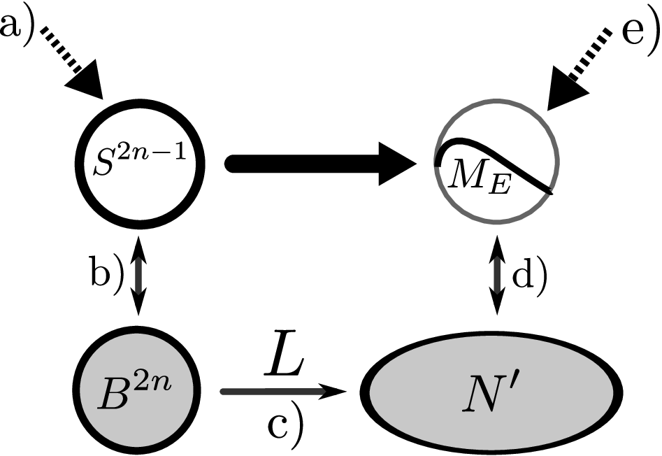
- a)
As explained at the beginning of this section, it is well-known how to pick random points approximately from the uniform distribution on the sphere : choose real and imaginary parts randomly, distributed independently identically according to a Gaussian distribution proportional to .
- b)
We have just seen that the uniform distribution in the ball and on the sphere are close to each other. Hence the algorithm from a) also samples the uniform distribution in the ball to good approximation.
- c)
Let be the full ellipsoid with equatorial radii
in the directions of the eigenvectors of , i.e.,
Then the ball and the ellipsoid are related by a linear transformation which preserves the normalized geometric volume measure: , then and .
Sampling the ball , and then applying the linear transformation , is the same as sampling the full ellipsoid . Writing , the components of vectors after the transformation are related to the components before by . Hence
Thus, we have shown that Algorithm 21 samples the full ellipsoid to good approximation.
- d)
The full ellipsoid is close the the full ellipsoid from Theorem 2. There, it was shown that the uniform volume measure in is close to the uniform measure on the energy manifold . Hence the uniform volume measure in is close to .
- e)
The sampling algorithm gives a simple method for a numerical check of identities such as the form of the reduced density matrix in Example 4. It is interesting to note that even though the typical reduced density matrices are not Gibbs states (cf. Theorem 5), the distribution involved in Algorithm 21 involves the Boltzmann-like term , where is constant, and denotes the -th energy level.
How good is the approximation given by Algorithm 21? As explained above, the algorithm is meant to approximate expectation values of functions on the energy manifold with respect to the measure . Thus, we would like to estimate the expression , where denotes the expectation value with respect to the Gaussian measure used in the algorithm. As a lower bound on that error (for some ), recall that
The function is Lipschitz continuous, and the upper bound on the Lipschitz constant on the unit ball does not grow with . Assume for simplicity that and are constant in (like in Example 3 and Example 4). Then
which shows that we have to expect at least an error of the order even for functions and Hamiltonians that behave very regularly.
A rough upper bound on the error can be given by adding the error contributions of steps a), b), c), and d) in Algorithm 21. It seems that the dominant contribution comes from step d) – a corresponding error estimate is given in Theorem 2. It is roughly of the order , again assuming that the energies and the Lipschitz constant are constant in .
VII Conclusions
In this work, we have established the notion of concentration of measure for quantum states with a fixed expectation value. The results that we established constitute on the one hand a new proof tool to assess properties of quantum states with the probabilistic method. Such a proof tool is expected to be helpful in a number of contexts, e.g., when sharpening counterexamples to additivity by enforcing a strong “conspiracy” by means of a suitable Hilbert Schmidt constraint, adding to the portfolio of techniques available related to the idea of a probabilistic method.
On the other hand, in this work we are in the position to introduce concentration of measure ideas to notions from quantum statistical mechanics, specifically to the mean energy ensemble, and link this physically meaningful ensemble to ideas of typicality. Obviously, a constraint of the type introduced here could as well relate to settings where the particle number is held constant, so is expected to be applicable to a quite wide range of physical settings. It is also the hope that methods similar to the ones established here also help assessing questions of typicality in the context of quantum dynamics and addressing key open problems in the theory of relaxation [15, 16, 17, 18] of non-equilibrium complex quantum systems.
VIII Acknowledgments
We would like to thank C. Gogolin and R. Seiler for discussions. This work has been supported by the EU (COMPAS, CORNER, QESSENCE, MINOS) and the EURYI.
References
- [1] N. Alon and J. H. Spencer, The probabilistic method (Wiley, 2000).
- [2] S. Lloyd and H. Pagels, “Complexity as thermodynamic depth”, Ann. Phys. 188, 186 (1988).
- [3] P. Hayden, D. Leung, and A. Winter, “Aspects of generic entanglement”, Commun. Math. Phys. 265, 95 (2006).
- [4] P. Hayden, D. W. Leung, P. W. Shor, A. Winter, “Randomizing quantum states: Constructions and applications”, Commun. Math. Phys. 250, 371 (2004).
- [5] M. Horodecki, J. Oppenheim, A. Winter, “Quantum information can be negative”, Nature 436, 673 (2005).
- [6] M. B. Hastings, “A counterexample to additivity of minimum output entropy”, Nature Physics 5, 255 (2009).
- [7] D. Gross, S. T. Flammia, and J. Eisert, “Most quantum states are too entangled to be useful as computational resources”, Phys. Rev. Lett. 102, 190501 (2009).
- [8] M. J. Bremner, C. Mora, and A. Winter, “Are random pure states useful for quantum computation”, Phys. Rev. Lett. 102, 190502 (2009).
- [9] S. Goldstein, J.L. Lebowitz, R. Tumulka, and N. Zanghi, “Canonical typicality”, Phys. Rev. Lett. 96, 050403 (2006).
- [10] S. Popescu, A.J. Short, and A. Winter, “Entanglement and the foundations of statistical mechanics”, Nature Physics 2, 754 (2006).
- [11] P. Reimann, “Foundation of statistical mechanics under experimentally realistic conditions”, Phys. Rev. Lett. 101, 190403 (2008).
- [12] C. Gogolin, “Einselection without pointer states”, arXiv:0908.2921.
- [13] M. Srednicki, “Chaos and quantum thermalization”, Phys. Rev. E 50, 888 (1994).
- [14] S. Garnerone, T. R. de Oliveira, and P. Zanardi, “Typicality in random matrix product states”, arXiv:0908.3877.
- [15] C. Kollath, A. Läuchli, and E. Altman, “Quench dynamics and non equilibrium phase diagram of the Bose-Hubbard model” Phys. Rev. B 74, 174508 (2006).
- [16] M. Rigol, V. Dunjko, V. Yurovsky, and M. Olshanii, “Relaxation in a completely integrable many-body quantum system: An ab initio study of the dynamics of the highly excited states of lattice hard-core bosons”, Phys. Rev. Lett. 98, 050405 (2007).
- [17] M. Cramer, C. M. Dawson, J. Eisert, and T. J. Osborne, “Exact relaxation in a class of non-equilibrium quantum lattice systems”, Phys. Rev. Lett. 100, 030602 (2008).
- [18] N. Linden, S. Popescu, A. J. Short, and A. Winter, “On the speed of fluctuations around thermodynamic equilibrium”, arXiv:0907.1267.
- [19] D. C. Brody, D. W. Hook, and L. P. Hughston, “Quantum phase transitions without thermodynamic limits”, Proc. R. Soc. A 463, 2021 (2007).
- [20] C. M. Bender, D. C. Brody, and D. W. Hook, “Solvable model of quantum microcanonical states”, J. Phys. A 38, L607 (2005).
- [21] B. Fresch and G. J. Moro, “Typicality in ensembles of quantum states: Monte Carlo sampling versus analytical approximations”, arXiv:0909.3175.
- [22] Z. Jiang and Q. Chen, “Understanding Statistical Mechanics from a Quantum Point of View”, in preparation.
- [23] H. Federer, Geometric measure theory (Springer-Verlag, 1969).
- [24] M. Ledoux, The concentration of measure phenomenon (Mathematical Surveys and Monographs 89, AMS, USA).
- [25] T. M. Cover and J. M. Thomas, Elements of information theory, Second Edition (Wiley, New York, 2006).
- [26] M. Gromov, Metric structures for Riemannian and Non-Riemannian spaces (Modern Birkhäuser Classics, 2007).
- [27] K. Zyckowski and H–J. Sommers, “Induced measures in the space of mixed quantum states”, J. Phys. A 34 No. 35, 7111 (2001).
- [28] M. Hall, “Random quantum correlations and density operator distributions”, Physics Letters A 242, 123 (1998).
- [29] R. Bhatia, Matrix analysis (Springer, 1997).
- [30] L. A. Santaló, Integral geometry and geometric probability (Addison-Wesley, 1972).
- [31] H. Tasaki, “Geometry of reflective submanifolds in Riemannian symmetric spaces”, J. Math. Soc. Japan 58 No. 1 (2006).
- [32] R. Schneider and W. Weil, Stochastic and integral geometry (Springer, 2008).
- [33] K. Funano, “Concentration of -Lipschitz Maps into an infinite dimensional -ball with the -distance function”, Proc. Amer. Math. Soc. 137, 2407 (2009).
- [34] K. Funano, “Observable concentration of mm-spaces into nonpositively curved manifolds”, Geometriae Dedicata 127, 49 (2007).
- [35] J. Elstrodt, Maß– und Integrationstheorie (Springer, 1996).
- [36] V. D. Milman and G. Schechtman, Asymptotic theory of finite dimensional normed spaces (Lecture Notes in Mathematics 1200, Springer, 2001).
- [37] L. E. Blumenson, “A derivation of -dimensional spherical coordinates”, American Mathematical Monthly 67, No. 1, 63 (1960).
- [38] I. Bengtsson and K. Zyczkowski, Geometry of quantum states - an introduction to quantum entanglement (Cambridge University Press, 2006).
- [39] A. P. Dempster and R. M. Kleyle, “Distributions determined by cutting a simplex with hyperplanes”, The Annals of Mathematical Statistics 39 5, 1473 (1968).
- [40] A. Barvinok, Measure concentration in optimization (Springer, 2007).
- [41] T. Furuta, “Short proof that the arithmetic mean is greater than the harmonic mean and its reverse inequality”, Mathematical Inequalities and Applications 8 4, 751 (2005).
- [42] M. E. Müller, “A note on a method for generating points uniformly on -dimensional spheres”, Comm. Assoc. Comput. Mach. 2, 19 (1959).
- [43] G. Marsaglia, “Choosing a point from the surface of a sphere”, The Annals of Mathematical Statistics 43 2, 645 (1972).