Dissertation
submitted to the
Combined Faculties of the Natural Sciences and Mathematics
of the Ruperto-Carola-University of Heidelberg. Germany
for the degree of
Doctor of Natural Sciences
Put forward by
Andreas Braun
born in Koblenz
Oral examination: February 5th, 2010
F-Theory and the Landscape of
Intersecting D7-Branes
| Referees: | Prof. Dr. Arthur Hebecker | ||
| Prof. Dr. Michael G. Schmidt |
Abstract
In this work, the moduli of D7-branes in type IIB orientifold compactifications and their stabilization by fluxes is studied from the perspective of F-theory. In F-theory, the moduli of the D7-branes and the moduli of the orientifold are unified in the moduli space of an elliptic Calabi-Yau manifold. This makes it possible to study the flux stabilization of D7-branes in an elegant manner. To answer phenomenological questions, one has to translate the deformations of the elliptic Calabi-Yau manifold of F-theory back to the positions and the shape of the D7-branes. We address this problem by constructing the homology cycles that are relevant for the deformations of the elliptic Calabi-Yau manifold. We show the viability of our approach for the case of elliptic two- and three-folds. Furthermore, we discuss consistency conditions related to the intersections between D7-branes and orientifold planes which are automatically fulfilled in F-theory. Finally, we use our results to study the flux stabilization of D7-branes on the orientifold using F-theory on . In this context, we derive conditions on the fluxes to stabilize a given configuration of D7-branes. This thesis furthermore contains an introduction to F-theory and a brief review of some mathematical background.
Chapter 1 Introduction
Unification has always been among the central themes of theoretical physics. String theory is one of the most ambitious projects in this development: it is aimed at nothing less than unifying all fundamental forces, including gravity, into a single theory. As all fundamental forces apart from gravity are quantum theories, this involves in particular giving a consistent quantum theory of gravitation. String theory is arguably the best-developed scheme for a theory with which this might be achieved.
In the last decade it was found that the five consistent superstring theories, all defined in ten space-time dimensions, are linked by an astonishing network of dualities. This lead to the conclusion that they are all limits of a single, more fundamental theory: M-theory (see e.g.[1]). In many cases, dualities open up completely new points of view and methods of computation. One of the most striking examples is given by the AdS/CFT correspondence [2]. On the mathematical side, dualities have inspired many far-reaching conjectures, the most famous example being homological mirror symmetry [3].
A fundamental challenge, which becomes even more pressing in the age of the LHC, is to connect string theory to existing models of particle physics and cosmology. Even though we seem to be holding a unique theory in our hands, this theory exists only in ten space-time dimensions. To remedy this problem one has to “compactify” string theory, so that only four dimensions, the ones we perceive, remain large. As superstring theory naturally incorporates supersymmetry (SUSY), one is hence tempted to aim for a supersymmetric version of the standard model, or some extension thereof. This choice has also a technical side: compactifications of string theory in which SUSY is broken at a low scale are under much better control than compactifications in which SUSY is broken at a high scale.
Compactifications of string theory involve the choice of a six-dimensional manifold. Even though the requirement of low-energy SUSY limits the choices that can be made to so-called Calabi-Yau manifolds, a huge freedom still remains. This freedom is further enhanced by the inclusion of so-called D-branes. D-branes are higher-dimensional objects which lead to gauge theories in the low-energy theory, see [4] for a review. As we are aiming for the gauge group of the standard model (or some GUT group), we are interested in studying compactifications with D-branes11 1 This is not the case in heterotic string theory, which has an or gauge theory already in ten dimensions. We discuss the dualities that connect compactifications of heterotic strings with compactifications of string theory with D-branes in various parts of this thesis.. Intersecting brane models are a promising candidate for constructing standard-like models [5].
String theory contains gravity in ten dimensions, which means that the ten-dimensional space-time is dynamical. Hence the manifold we have compactified string theory on will be dynamical as well. Without further input, the deformations of this manifold have no potential and give rise to massless scalar fields in four dimensions, called moduli. As D-branes are dynamical objects, they contribute further moduli, the study of which is one of the main topics of this work. Moduli are a phenomenological disaster because they mediate interactions that are comparable to gravity in strength and thus spoil the equivalence principle. We will refer to this as the moduli problem of string compactifications.
Fortunately, string theories contain further ingredients which solve the moduli problem in a natural way. The crucial ingredient are so-called fluxes, background values of -form fields along the compact directions. These fluxes have to obey quantization conditions similar to Dirac monopoles, and can only exist along non-trivial homology cycles of the compactification manifold. There has been a large amount of work devoted to the study of compactifications with fluxes in recent years, see [7, 8, 6, 9] for reviews. In particular, it has been realized that the potential which is generated by the energy density of the fluxes is capable of fixing geometric as well as D-brane moduli, hence solving the moduli problem. In this work, we use a framework called F-theory to study the flux stabilization of D7-branes22 2 A D-brane extends in spatial directions, so that it is a -dimensional object in space-time. in compactifications of type IIB string theory in detail.
From the perspective of the underlying physics, the choice of fluxes and the inclusion of D-branes is very similar to the choice of a compactification manifold. On the one hand, all three involve a choice for the background value of some degrees of freedom. If we allow ourselves to choose a background value for the space-time metric such that six dimensions are compact, we might as well allow background values for other degrees of freedom. In fact, it would seem unnatural not to. On the other hand, the actual choices we have to make to specify the compactification manifold, fluxes and D-branes are all discrete. Once a manifold with D-branes and fluxes is chosen, the flux potential, together with a contribution from non-perturbative effects, will fix the geometric moduli and the positions and shapes of the D-branes.
1.1 The string theory landscape
The topology of the compactification manifold, D-branes and the fluxes allow, in principle, to compute the complete low-energy spectrum including all coupling constants. The effective four-dimensional theories one obtains are hence parameterized by the values of a set of integers. The number of possible effective theories can be obscenely large, with rough estimates leading to numbers such as [10]. All of these compactifications correspond to valid solutions of string theory.
Compactifications of string theory on different manifolds are not as distinct as it may seem at first. In fact, there can be transitions between topologically different Calabi-Yau manifolds. Geometrically, these transitions involve deforming a Calabi-Yau manifold until a singularity develops and subsequently resolving this singularity such that one ends up with a topologically different manifold. It turns out that this process is, however, perfectly well-behaved in string theory, see e.g. [12, 11]. Even though there is no general proof of the conjecture that all Calabi-Yau spaces are connected by such singular transitions33 3 This idea is goes back to the mathematician Miles Reid and is sometimes called “Reid’s phantasy” [13]., all examples that are known so far are part of a gigantic web [14, 15]. Similar insights have been obtained regarding D-branes and fluxes [16]. Hence different flux compactifications with D-branes should be properly viewed as different vacua in the “landscape” of all string compactifications.
As we have discussed, the uniqueness of string theory in ten dimensions is lost upon compactification. Instead, there is a (possibly finite) discretuum of string vacua in four dimensions. This result can be interpreted in a number of ways. One approach is to postpone worries about uniqueness until one has constructed a string compactification which is consistent with experiments. This is a difficult task and much of the work in string phenomenology has been following this path. Another conclusion one might draw is that we have not properly understood string theory yet. A logical possibility is that we are missing a fundamental principle which can tell us how to single out one specific compactification, which then, hopefully, reproduces the Standard Model of particle physics as its low-energy description.
The point of view which is the basis for this work, is to accept the existence of the multitude of string vacua as a fundamental feature of string theory, see [17] for an early proposal of this idea. Conceptually, a good analogy for the state of affairs is given by chemistry [18]. Even though there are only three building blocks, neutrons, protons and electrons, there are many stable (or metastable) vacua: atoms. A crucial difference is, of course, that we can observe many different atoms, including excited states, in nature, whereas other string vacua seem practically inaccessible to us.
The general idea to handle such a landscape of string vacua is hence to look for correlations between aspects of the emerging low-energy theories and compare the findings to established experimental facts. Investigations of this sort were pioneered in [19, 20, 21], see also [6, 24] for reviews. In the context of intersecting D-brane models on toroidal orientifolds, a statistical study has been performed in [22, 23].
The picture of the landscape of string vacua we have drawn has an interesting interplay with cosmology. As the different vacua can be connected by tunneling, or decay into each other, the landscape can become populated statistically in the evolution of the early universe. This offers solutions to several cosmological problems, see e.g. [25] and [26]. One of the most prominent cosmological problems that can be addressed in flux compactifications is the cosmological constant problem. As has been proposed in [27], the cosmological constant, being equal to the energy density of the vacuum, can be small due to cancellations among the many possible fluxes.
The vacuum energy for supersymmetric compactifications, however, is always non-positive. Hence a positive cosmological constant can only be obtained after SUSY is broken. It has been shown in [28] (see also [29] for a summary) that this can be achieved in a controlled way in the setting of flux compactifications of type IIB string theory, to be discussed below. The SUSY-breaking metastable minimum one obtains have a tunably small positive cosmological constant.
The complicated effective potential that arises in the string landscape is also an ideal playground for implementing models of inflation, see [30] for a review. There is growing evidence that the number of meta-stable string vacua which are compatible with very general properties of the Standard Model (minimal mass for lightest Kaluza-Klein excitations, small positive cosmological constant, not too large extra-dimensions) is finite [31].
Flux compactifications on Calabi-Yau manifolds generically contain so-called throat geometries which describe strongly warped regions [32]. The magnitude of the warping, which gives rise to large hierarchies of mass-scales from the 4-dimensional perspective, depends on the ratio of certain flux numbers [33]. (This can be mapped fairly explicitly [34, 35, 36] to the famous 5-dimensional model of Randall and Sundrum [37], which explains the hierarchy between the electroweak and the Plank scale.) A statistical analysis shows that throats are generically expected in compact spaces with many cycles [38].
1.2 Type IIB orientifold compactifications and F-theory
One of the best-understood branch of the string theory landscape is provided by Calabi-Yau orientifold compactifications of type IIB string theory with D3 and D7 branes. This is also the framework in which most of the ideas presented above were implemented. In this section, we only give some details related to this work, see [8, 6, 24] for a thorough introduction to type IIB orientifolds.
At low energies, type IIB string theory is well described by the ten-dimensional type IIB supergravity [1]. The bosonic field content of type IIB supergravity splits into the Neuveu-Schwarz (NS-NS) and the Ramond-Ramond (R-R) sector. In the Neuveu-Schwarz sector there is the metric , the dilaton , a 2-form potential . The 2-form gives rise to a 3-form field-strength . The Ramond-Ramond sector contains the -form potentials , . The exterior derivatives of the forms yield the field strengths . The five form furthemore has to fulfill the self-duality condition , where denotes the Hodge- operation. For convenience we introduce the fields
| (1.1) |
The bosonic equations of motion of type IIB supergravity can be derived from the action
| (1.2) |
supplemented by . As the self-duality makes the kinetic term of vanish, it can only be enforced at the level of the equations of motion. We have used units in which the string length, which is related to the string tension by , is set to unity.
Type IIB string theory contains D-branes of all even dimensions. Their effective action consists of two pieces, one of which, the so-called Dirac-Born-Infeld action, describes their dynamics and the gauge theory living on their worldvolume. The remaining piece, the Chern-Simons action, describes the coupling of a D-brane to the various Ramond-Ramond fields of string theory [4]:
| (1.3) |
In the above equation we have abbreviated , where and . Furthermore, denotes the Chern class and is the -roof genus, see Appendix A.1. The 2-form of the gauge theory living on the worldvolume of the D-brane is denoted by . and denote the tangent and normal bundle of , respectively. The integrand in the expression above only makes sense when expanded in terms of the various differential forms that appear in it. The integral then picks out those forms matching the dimension of the D-brane. Note that the Chern-Simons action of a D-brane contains a term
| (1.4) |
Hence a D-brane sources the field . In this sense, the Chern-Simons action is a generalization of the coupling of a point-particle to the electromagnetic potential.
Taking the quotient of type IIB string theory on a Calabi-Yau manifold by
| (1.5) |
produces a so-called orientifold compactification. Here denotes the parity transformation on the string world-sheet, is the left-moving fermion number on the world-sheet and is a holomorphic involution of the Calabi-Yau manifold which projects out the holomorphic 3-form . The geometric quotient of the Calabi-Yau by is hence no longer Calabi-Yau. Compactifications of type IIB string theory on Calabi-Yau manifolds have SUSY in four dimensions. Orientifolding reduces the supersymmetry further to . The action of on the fields of type IIB supergravity is
| (1.6) |
String theory compactifications must obey certain consistency conditions, which are known as the tadpole cancellation conditions. They originate from Gauss’ law for the charges (which correspond to various differential forms) induced by D-branes and fluxes, applied in a compact geometry. From the point of view of string theory, the tadpole cancellation conditions guarantee the absence of anomalies. To cancel the charge of D7-branes, compactifications of type IIB string theory must contain orientifold 7-planes (O7-planes). O7-planes are given by the fixed locus of the involution . They are lie at the fixed-point locus of a holomorphic involution, so that they are locally given by the vanishing of holomorphic function.
The coupling of orientifold planes to the fields of type IIB supergravity can also be described by an action similar to (1.3). Denoting the worldvolume of an O-plane by , it is given by [4]
| (1.7) |
In the above equation, denotes the Hirzebruch -genus, see Appendix A.1. The coupling of an O-plane to is hence
| (1.8) |
This is the same as the coupling of a D-brane except of a factor of and a minus sign. This sign is crucial for the cancellation of the charges between D-branes by O-planes. For O7-planes and D7-branes, the relative factor is . In the double cover, we hence need to have eight times as many D7-branes as O7-planes to cancel their charges. After orientifolding, only half of the D7-branes are present. Denoting the homology class of all the O7-planes in the quotient by , the homology class of all D7-branes must hence be to cancel the D7-brane tadpole. Hence we cannot simply add D7-branes to a compact Calabi-Yau compactification as they can only be consistently included in type IIB orientifolds44 4 It is possible to include D7-branes even in the absence of O7-planes in non-compact models. Note that this means in particular that the total homology class of all D7-branes is fixed.
In order not to spoil Lorentz invariance in the effective four-dimensional theory, we need all D-branes to fill out all four non-compact dimensions. This means that D3-branes are points in the six compact directions, whereas the D7-branes extend in four compact directions. As we need the right O-planes to cancel the charges of the D7-branes, a consistent model should contain O7-planes which also fill out the four non-compact directions and have the real codimension two in the six compact dimensions. The involution should hence have a fixed point locus which has codimension two in the compact geometry. As the involution is furthermore required to be holomorphic, the O7-planes are given by divisors of the Calabi-Yau manifold.
The simplest way to cancel the D7-brane tadpole is to place four D7-branes on top of the O-plane. When one moves the D7-branes off the O7-plane, supersymmetry requires them to be given by the vanishing of holomorphic functions on . Hence both the O7-planes and the D7-branes are described by divisors.
Let us briefly review some aspects of the moduli of such compactifications, see also [39, 40]. The moduli of Calabi-Yau threefolds split into Kähler and complex structure moduli, see Appendix A.4.6. These can be thought of as variations of the Kähler form and the holomorphic 3-form , respectively, see Appendix A.4.6. In particular, complex structure moduli can be expressed in terms of the periods
| (1.9) |
where the are elements of the third homology group of the Calabi-Yau manifold.
As is odd and is even under , we find that Calabi-Yau orientifolds have Kähler and complex structure deformations. Whereas each complex structure deformation corresponds to a complex degree of freedom, the bosonic field content of a chiral multiplet, there is only one real degree of freedom associated with each Kähler deformation. In the four-dimensional effective theory, the Kähler moduli pair up with the zero modes of the two form to form the bosonic components of chiral multiplets55 5 Although these moduli can be naturally included in linear multiplets, one usually dualizes them to chiral multiplets, see [39].
As D7-branes are submanifolds of , one expects their deformations to be given by sections of their normal bundle [40]. As we discuss in Section 4.4.1, D7-branes are not completely generic hypersurfaces, but have obstructed deformations due to the presence of the O7-plane. They are forced to take a shape such that all intersections between the D7-branes and the O7-planes are double intersections. We discuss how this arises by using the weak coupling limit of F-theory in Section 2.4.4. As has been discussed in [41], this can also be seen in perturbative type IIB string theory.
Due to the curvature terms in (1.3) and (1.7), D7-branes and O7-planes contribute to the D3-brane tadpole. This contribution can be cancelled by either introducing D3-branes or 3-form fluxes , which contribute to the D3-brane tadpole due to the coupling in the type IIB supergravity action.
It has been shown in [33], that one can switch on 3-form fluxes in type IIB orientifolds preserving SUSY. The geometry of these models is, up to warping, still described by a Calabi-Yau orientifold. These fluxes are capable of fixing all the complex structure moduli. This is described by the Gukov-Vafa-Witten superpotential:
| (1.10) |
This superpotential can be easily translated into an effective potential for the periods, (1.9). We have drawn a cartoon of a flux compactification in Figure 1.1
The remaining Kähler moduli can be fixed by 2-form fluxes on the D-branes and non-perturbative effects, such as gaugino condensates. As has been argued by [28], these models can have metastable de Sitter vacua in which SUSY is broken. Furthermore, one can show that the moduli of D-branes are fixed by fluxes as well, see e.g. [42, 43]. An explicit picture of this, however, is lacking except for simple examples [44, 45, 46].

D7-branes and O-planes couple to the form via (1.4) and (1.8). As , they magnetically source . This means that compactifications in which we displace D-branes from the O-planes necessarily have a non-constant axiodilaton. The equations of motion force to be a holomorphic function of . This means that undergoes upon encircling a D-brane and upon encircling an O-brane. Because type IIB has a self-duality, there can be consistent solutions in which the D7-brane charge is not cancelled locally. This maps
| (1.11) |
so that in particular and are identified. The corresponding solutions are the similar to the backgrounds one obtains for cosmic strings [47], which also are codimension-two objects (in four dimensions).
Backgrounds with varying dilaton are most naturally described by F-theory. The idea leading to F-theory is to interpret as the complex structure modulus of a torus [48]. This is a natural identification, because two tori that have complex structure moduli connected by an transformation are diffeomorphic as complex manifolds [49, 50]. One way to see this is the construction of a torus as a quotient of . One identifies , so that any two tori that come from equivalent lattices are also equivalent. Two such lattices are isomorphic if they are related by an transformation. Interpreting as the modular parameter of an extra torus geometrizes the duality group of type IIB string theory. As is a holomorphic function of the coordinates of the Calabi-Yau orientifold , there is a torus over every point of which varies holomorphically. This is called an elliptic fibration. The way this torus is fibred over the base space encodes the positions of the D7-branes and O7-planes. In particular, the fibration is non-trivial due to the fact that the fibre torus degenerates over the positions of the branes, see Figure 1.2 There is a map which relates degenerations of the fibre torus to the gauge symmetry of the corresponding branes. We give an introduction to elliptic fibrations in Section 2.2.

The fact that D7-branes are (real) codimension-two objects makes them backreact strongly on the geometry, i.e. there is no probe approximation and their presence can be inferred also from great distance [47, 51]. This effect is automatically taken into account by requiring the total space of the fibration of the torus over to be a Calabi-Yau manifold .
The moduli space of this Calabi-Yau manifold encodes the moduli space of plus the moduli of the fibration of the over . As the details of the fibration are determined by the positions of the D7-branes and O7-planes in , the moduli space of this Calabi-Yau manifold unifies the moduli space of a Calabi-Yau orientifold with the moduli space of the D7-branes wrapped on its 4-cycles. Another advantage of this description is that constraints such as double intersections between O-planes and D-branes are naturally incorporated in this framework. Recombinations of D-branes, processes in which the intersection between two branes is smoothed out such that a single brane results, can also be easily described within this framework. In particular, we show that recombinations are related to shrinking cycles of the elliptic Calabi-Yau manifold of F-theory in Section 4.1.
A large part of this thesis is devoted to the question of how complex structure moduli of elliptic Calabi-Yau manifolds encode the positions and the shape of D7-branes and O7-planes. As complex structure moduli of Calabi-Yau manifolds come from cycles of the middle homology (see Appendix A.4.6), our strategy is to analyse how these cycles arise from the topology of the D7-branes and O7-planes. Using the details of the elliptic fibration over , we show how this can be achieved for elliptic surfaces and Calabi-Yau threefolds, i.e. for a complex one- and two-dimensional base space . Related work using different techniques recently appeared in [52].
Even though the fibre torus may seem like an auxiliary concept, it becomes quite real in the dual M-theory description: type IIB orientifolds on are dual to M-theory on in the limit in which the size of the fibre torus goes to zero [53]. This is called the F-theory limit.
From our perspective, the real power of the F-theory description is that we can describe flux compactifications from the perspective of M-theory. As 11-dimensional supergravity contains a 3-form potential, one can switch on 4-form flux in M-theory backgrounds. Under the duality to type IIB, the flux is mapped to both flux and gauge flux on the branes. Compactifications of M-theory on elliptic fourfolds [54] with 4-form flux share many of the good properties of type IIB flux compactifications: The geometry is, up to warping, still Calabi-Yau in the presence of fluxes [55] and the potential generated by the fluxes [57, 56] is capable of fixing all the complex structure moduli. Similar to type IIB flux compactifications, moduli stabilization is best described by writing the flux potential in terms of the periods. As the periods of F-theory compactifications on elliptic fourfolds determine the position and shape of D7-branes and O7-planes, this approach allows us to study flux stabilization of D-branes [59, 58]. An understanding of the map between periods of elliptic Calabi-Yau manifolds and the D-brane configurations they describe hence allows a very explicit study of D-brane stabilization by fluxes. This is our main motivation for working out how the cycles of elliptic Calabi-Yau manifolds are related to deformations of D7-branes and O7-planes. We give an example of this approach in Chapter 5: we show how to use the map between cycles and D7-brane positions to work out flux stabilization of D-branes on the orientifold which is described by in F-theory.
F-theory can also be thought of as a non-perturbative description of type IIB backgrounds. One way to see this is to note that the self-duality group which is used in F-theory contains strong-weak coupling transitions. Hence there can be compactifications of F-theory which inevitably contain regions where the coupling is strong. Correspondingly, F-theory vacua can contain branes and couplings which are absent in perturbative type IIB string theory. In agreement with the interpretation of singularities of the elliptic fibration as gauge groups of the corresponding branes, those objects can support gauge theories with exceptional gauge groups on their worldvolume. In the context of GUT model-building, this has recently attracted a lot of attention [61, 62, 60, 63, 64]. In perturbative type IIB compactifications with D-branes, one needs instanton effects to generate the right Yukawa couplings, e.g. the coupling in GUTs [65]. In GUTs based on F-theory, these couplings can come from singularities that are of type. Other advantages include a natural mechanisms for the breaking of the GUT gauge group down to the standard model and for the generation of the hierarchy between th GUT and the Planck scale. Furthermore, one can engineer the absence of higherdimensional operators that lead to Proton decay by choosing the geometry appropriately. For a study of SUSY-breaking in these models, see [66, 67, 68]. Until recently, most of the work on F-theory GUTs has focussed on the study of desirable effects in local models. Studies of global compactifications include [69, 70, 71]. For the F-theory versions of perturbative type IIB GUT models see [73, 72].
1.3 Overview
In Chapter 2 we give an introduction to F-theory and elliptic fibrations. We introduce the Weierstrass model description and discuss how various stacks of branes are encoded in the elliptic fibration. We mainly focus on the weak coupling limit, in which F-theory describes perturbative IIB orientifold compactifications.
After the first chapter we start with the main part of this thesis, which contains our own work. In Chapter 3, which is based on [74, 75], we treat F-theory on elliptic surfaces in detail. is the only non-trivial compact two-dimensional Calabi-Yau manifold, so that it represents the simplest non-trivial F-theory compactification. We start this section with a review of the properties of elliptic surfaces, which have a two-sphere as their base space. The enhancement of gauge symmetry which occurs for coincident D-branes can be beautifully mapped to singularities of . This is also evident from the duality to the heterotic string, which we discuss in detail. We then show how to construct the second homology group of from the presence of D7-branes and O7-planes. In other words, we explicitly understand the motion of the 16 D7-branes the background geometry in terms of shrinking or growing cycles stretched between the branes or the orientifold planes. We then discuss the relation of a described by a Weierstrass model at the orientifold point to . Even though these spaces are different, they describe the same F-theory background. We discuss an intuitive way to deform these spaces into each other and show that they approach the same space in the F-theory limit. We also provide an example, given by the Enriques involution, which shows that there can be symmetries which are only present in the F-theory limit in the Weierstrass model description.
In Chapter 4, we study the moduli D7-branes and O7-planes of F-theory compactifications on elliptic three-folds from the perspective of complex structure deformations. This chapter is based on [76]. Working in the weak coupling limit, we construct 3-cycles from the topology of the D-branes and O-planes. We achieve complete agreement between the degrees of freedom encoded in the Weierstrass model and the complex structure deformations of the elliptic Calabi-Yau threefold. All relevant quantities can be expressed in terms of topological quantities of the base space, allowing us to formulate our results for general base spaces. Furthermore, we discuss in detail how the degrees of freedom of D7-branes are restricted as compared to generic hypersurfaces.
In Chapter 5, we consider the stabilization of M-theory on in the presence of fluxes. Given a certain flux which is consistent with the F-theory limit, we can explicitly derive the positions at which D7 branes or stacks of D7 branes are stabilized. Our analysis is based on a parameterization of the moduli space of type IIB string theory on (including D7-brane positions) in terms of the periods of integral cycles of M-theory on , obtained in Chapter 3. This allows us, in particular, to select a specific desired gauge group by the choice of flux numbers. This chapter is based on [77].
The appendix contains an introduction to some of the mathematics used throughout this work.
Chapter 2 Aspects of F-theory and elliptic fibrations
In this chapter we review F-theory and explain the geometrical constructions that are needed. Some of the underlying mathematics is presented in the appendices. Our exposition mostly focuses on topics and methods that are directly relevant to the subsequent chapters, see [24, 78] for recent reviews of similar material.
2.1 Type IIB and
The type IIB string theory has an self-duality. In the ten-dimensional IIB supergravity action this shows up as an which acts on the complexified string coupling , also known as the axiodilaton, and the NS-NS and R-R 2-forms as
| (2.1) |
and leaves invariant. On the quantum level, quantization of the field-strengths associated to the 2-forms degrades the symmetry to . Its nonperturbative nature is apparent from the fact that it exchanges the field strength coupled to the fundamental string with the field strength of a D1 brane, a non-perturbative object. This goes along with an exchange of strong and weak coupling, and is generated by the element (for )
| (2.2) |
F-theory [48] describes type IIB backgrounds which are patched together using this self-duality. This construction is inevitable in the presence of D7-branes and orientifold 7-planes (O7-planes) as they are magnetically charged under the real part of . Upon encircling11 1 As these objects have real codimension 2 in a 10-dimensional spacetime, there is a well-defined notion of a winding number. a D7-brane we have that . The corresponding element of is commonly denoted by22 2 The two elements actually generate the whole group . Given their physical interpretation this means that all type IIB vacua with varying coupling are built out of D-branes and strong weak coupling transitions. This observation will be made more precise later on.
| (2.3) |
For O7-planes, the action on is given by . The corresponding element is however not simply , but . Altough the extra minus sign acts trivially on , its presence can be inferred from the orientifold action on the 2-form fields.
Supersymmetry requires to be a holomorphic function of the base. From this it follows that the torus degenerates such that at the positions of the D-branes. This is best described by using the modular function instead of itself. The function is a holomorphic bijection from the fundamental domain of (see Figure (2.1)) onto the Riemann sphere and is invariant under transformations of (details can be found in [50]).

The fundamental domain contains three singular points which are fixed points under a subgroup of . These points and the generators of this subgroup are33 3 We have chosen a normalization of Klein’s -function that agrees with the convention used in the physics literature [79].
| invariant under | ||
|---|---|---|
| 0 | ||
| . |
Whenever encircles one of these three points, undergoes the corresponding transformation.
A very elegant way to describe how type IIB backgrounds with varying string coupling are patched together is to interpret as the complex structure modulus of an extra torus. This torus does not describe further dimensions of space-time, but rather gives a geometrization of backgrounds with varying axiodilaton . This is the basic idea of F-theory. In this picture, the is the monodromy group acting on the 1-cycles, and thus on the complex structure modulus, of the fibre torus. The tori can be patched together because two tori which have a complex structure modulus related by an transformation can be mapped holomorphically to one another. As the complex structure modulus of the extra torus is used to describe the axiodilaton, its volume is of no physical importance.
From this point of view, F-theory is a description of type IIB backgrounds with D7-branes which is obtained by holomorphically fibering a torus over spacetime. The monodromies acting on this torus encode the positions (and type) of the D-branes. The spaces one obtains in this way are called elliptically fibred manifolds, and we will review their properties and construction in the next section. We will finally be interested in elliptically fibred Calabi-Yau manifolds [79].
2.2 Elliptic fibrations
An elliptic fibration is a space together with a holomorphic map (the projection) to a space (the base), such that the generic fibre, , is a non-singular elliptic curve, also known as a torus.
![[Uncaptioned image]](1003.4867v1/ellfib.png)
Elliptic fibrations may have a section , which is a map from the base into the total space such that intersects each fibre once.
![[Uncaptioned image]](1003.4867v1/ellfibs.png)
We can also have n-sections, in which case the section intersects each fibre n-times.
Let us introduce the so-called Weierstrass model description:
| (2.4) |
There is a very intuitive way to understand this equation. For every point of the base it describes a double cover of the Riemann sphere, branched over four points: the three roots of the right hand side plus the point at infinity. Hence it describes a torus, which varies its shape when we change the point on the base.
![[Uncaptioned image]](1003.4867v1/dct2.png)
For our purposes, it will be of advantage to slightly rewrite the Weierstrass equation so that it describes the elliptic fibre as hypersurface in weighted projective space.
| (2.5) |
We take to be the homogeneous coordinates of a bundle44 4 One can also use other spaces for embedding the fibre and in this way finds elliptic fibrations which allow for more than one section [80]. These fibrations do not have the full monodromy group [81], allowing a non-zero -field invariant under S-duality to be switched on. This can be exploited to construct F-theory duals to the CHL string [82]. over . The bundle over the base is such that is a section of and is a section of , for an appropriate line bundle . It follows that and are sections of and , respectively. If we take e.g. the projective space as the base, all this boils down to letting and transform under the scaling of and making and homogeneous polynomials such that (2.5) is a homogeneous equation with respect to a bundle over . A similar construction applies if is any toric variety. An elliptic fibration described by (2.5) hence is given by a hypersurface in a bundle over the base if is a toric variety. Thus one can use all the standard techniques to analyse it, see e.g. Appendix A. This can be generalized to situations in which the base itself is a hypersurface or complete intersection, see [83] for the details.
Let us fix some point in the base. In this case (2.5) is a homogeneous equation of degree 6 in . The singularities of are located at and . As is not part of , the space described to (2.5) always misses these singularities. Bertini’s theorem [84], see also Appendix A, then ensures that is generically a smooth space if and are sufficiently generic.
The first chern class of is readily computed. Denoting the hyperplane divisor of , which is given by by we find that
| (2.6) |
Hence
| (2.7) |
Thus for fixed point in the base, (2.5) describes a one-dimensional Calabi-Yau space, also known as a torus. The projection is now given by simply forgetting about the coordinates . The section of this fibration is found by mapping any to the point . Using the scaling of one can check that the equation has actually only one solution. This single point is the intersection between the section and every fibre. The obvious trick here is that eliminates any dependence on the base.
In application of elliptic fibrations to F-theory one is usually interested in a fibration such that the surface described by (2.5) is Calabi-Yau. This requirement can be seen from a number of perspectives that will be explained when we come to the physics of F-theory on elliptic fibrations. Let us denote the divisor associated to the bundle by . Using the second adjunction formula, (A.63), the Chern class of is
| (2.8) |
so that the condition for the first Chern class of to vanish is
| (2.9) |
Thus has to be equal to the anticanonical bundle for (2.5) to describe a Calabi-Yau manifold.
Choosing is the easiest example. As , where is the hyperplane divisor, the anticanonical bundle must vanish on two points of . Thus its sections are given by homogeneous polynomials of degree two. To get a Calabi-Yau space, we thus need to choose and to be homogeneous polynomials on of degree and , respectively:
| (2.10) |
The weights of the projective coordinates are given by
| 3 | 2 | 1 | 0 | 0 | |
| 6 | 4 | 0 | 1 | 1 | . |
As there is only one non-trivial Calabi-Yau manifold in two complex dimensions, (2.10) describes an elliptic surface, an object that will reappear frequently throughout this work.
As a second example, consider . Now we find that , where is the hyperplane divisor of and is the hyperplane divisor of . The sections of are thus given by homogeneous polynomials that have the bidegree . We can write our Weierstrass model,
| (2.11) |
where the weights of the projective coordinates are given by
| 3 | 2 | 1 | 0 | 0 | 0 | 0 | 0 | |
| 6 | 4 | 0 | 1 | 1 | 0 | 0 | 0 | |
| 9 | 6 | 0 | 0 | 0 | 1 | 1 | 1 | , |
and the degrees of homogeneity of and are as indicated. Using the methods explained in the appendix, one can check that the two examples are indeed Calabi-Yau. For every equivalence relation, the sum of the weights of all projective coordinates must equal the degree of the equation defining the hypersurface.
In our general discussion we have assumed that actually has holomorphic sections and (2.5) describes a smooth space. This can seen to be true without much work for the two examples. It is intuitively clear that the construction presented demands the bundle to be “positive” in some sense. A more precise rephrasing of this criterion is the concept of ampleness, as described in the appendix. Spaces with an ample anticanonical bundle are called Fano varieties and have been classified in dimensions up to three [85]. The toric fano threefolds have recently been discussed in the physics literature in [86].
2.2.1 Topological invariants
Given a base , there is only one choice for the bundle such that (2.5) yields an elliptic Calabi-Yau manifold: . This allows to derive expressions for its characteristic classes in terms of the characteristic classes of the base, which are often called Sethi-Vafa-Witten formulae [87].
Elliptic Calabi-Yau twofolds are always elliptic surfaces. Hence their Euler characteristic is always given by .
For the case of elliptic threefolds, we use the trick of [87]. As the whole structure of the elliptic threefold is fixed once the Chern classes of the base are known, we expect that we can write the Euler characteristic of an elliptic threefold over as an integral of the Chern classes of . Furthermore, the elliptic fibration is trivial if and only if , so that the expression for the Euler characteristic of must be proportional to . Hence we make the Ansatz
| (2.12) |
To determine the constant we consider an example, . As , where denotes the hyperplane divisor, we find that . Furthermore, we can compute the Euler characteristic of by considering a Calabi-Yau hypersurface in the toric variety given by the weights
| 3 | 2 | 1 | 0 | 0 | 0 | |
| 9 | 6 | 0 | 1 | 1 | 1 | , |
where are the homogeneous coordinates on . The Euler characteristic of this hypersurface Calabi-Yau can be computed by integrating the top Chern class of , see Appendix A.4.6 for similar examples. In the present case, the result is . Hence we find , so that we have found
| (2.13) |
We can use the same strategy to compute the Euler characteristic of an elliptic fourfold by intergrating the Chern classes of the base. The result is [87]
| (2.14) |
2.3 Monodromy and singularities
The -function of the torus fibres is given in terms of and as
| (2.15) |
As for it follows that the fibre degenerates over those points of the base, where the discriminant vanishes. These are the locations of the 7-branes of F-theory.
We can also understand this in a second way by directly checking when the torus becomes singular. Writing, for a fixed point in the base,
| (2.16) |
one can check that
| (2.17) |
so that the fibre torus degenerates if and only if . The difference between the roots on the right hand side are nothing but the positions of the branch points, if one thinks of the torus as a double cover over . As the distances between the branch points give the sizes of the 1-cycles of the torus, the singularities that arise when the branch points coincide develop because a 1-cycle of the torus is pinched. In the mathematics literature, is referred to as a vanishing cycle.
The relation between the vanishing cycle and the action on a 1-cycles of the torus upon encircling the locus is given by the Picard-Lefschetz monodromy formula [88, 89],
| (2.18) |
Here denotes the intersection form. Let us choose a basis for the 1-cycles of a torus and call the horizontal 1-cycle and the vertical 1-cycle , see Figure 2.2.

We choose the orientation such that . If the cycle vanishes, an arbitrary cycle undergoes the monodromy
| (2.19) |
when it is transported around the singularity. As expected, the transformation is given by an matrix. A consequence of the fact that monodromies are linked to vanishing cycles is that monodromies are only defined locally. Let be the cycle that vanishes at the point and the corresponding monodromy. If we now encircle another point , at which another cycle vanishes, the cycle is transformed to
| (2.20) |
Correspondingly, the monodromy matrix is changed to , where is the monodromy matrix associated with the vanishing of the cycle . Thus monodromies are only defined up to conjugation globally. If two vanishing cycles fulfill the relation
| (2.21) |
they are said to be mutually local. If this condition is met, the map (2.20) acts as the identity, so that the two monodromies are, in a sense, independent.

Note that the functional dependence of the -function on the base, (2.15), is such that all monodromies locally are some power of or [92]. By Table 2.1, monodromies that are different from can occur whenever is or . As near , the monodromy is not but . Similarly, in the vicinity of is given by
| (2.22) |
so that the monodromy around is .
2.3.1 Elliptic Surfaces
Let us first discuss the case of elliptic surfaces as it contains (almost) all the salient ingredients. For F-theory compactifications we are thus talking about elliptic surfaces, as described by (2.10). The following analysis will not depend on this, however, as only local properties are relevant.
The types of singular fibres that can occur for elliptic surfaces have been classified by Kodaira [90, 88]. The type of singular fibre only depends on the vanishing degree of , and . The fibre singularities can be directly translated to singularities of the complex surface, as is indicated in Table 2.2.
| fibre type | singularity type | monodromy | |||
|---|---|---|---|---|---|
| smooth | none | ||||
| none | |||||
Note that the monodromies are local, i.e. only determined up to -equivalence.
As an example we discuss the case of an fibre in some detail. The according monodromy is , so this configuration describes two coincident D7-branes (see Section 2.1). At a point where the fibre degenerates, two of the coincide so that, adjusting the normalization for convenience, the Weierstrass model locally reads
| (2.23) |
To see what happens to the whole space we have to keep the dependence on the base coordinates. Let us deform away from the degenerate point by shifting . This means that now
| (2.24) |
The quadratic difference of the now indegenerate roots is given by
| (2.25) |
Comparing this with (2.17) and ignoring the slowly varying factor associated with the distant third root, we have
| (2.26) |
Since we also want to see what happens to the full space, let us reintroduce the dependence on the base coordinates, , and write (2.24) as
| (2.27) |
Without loss of generality we assume and use as an affine coordinate. Near the fibre we can write , so that the Weierstrass model reads
| (2.28) |
By computing the gradient, one quickly sees that the above equation describes a singular hypersurface. This analysis can easily be modified to see that simple roots of do not lead to any singularity of the whole space, whereas higher roots lead to singularities in accordance with Kodaira’s classification.
We can resolve this singularity in two ways, both of which will make a two-sphere emerge.
Deformation
Let us first do the obvious and deform it to
| (2.29) |
where is some complex parameter.
As the situation is somewhat analogous to the conifold case [93], we will essentially repeat the analysis that is done there: We first note that can always be chosen to be real by redefining the coordinates. Next, we collect in a complex vector with real part and imaginary part . The hypersurface (2.29) may then be described by the two real equations
| (2.30) |
We can understand the topology of X by considering its intersection with a set of 5-spheres in given by , :
| (2.31) |
If we assume for a moment that , the equations above describe two s of equal size for every that are subject to an extra constraint. If we take the first to be unconstrained, the second and third equation describe the intersection of another with a hyperplane. Thus we have an bundle over for every finite . This bundle shrinks to zero size when approaches zero so that we reach the tip of the cone. Furthermore, the bundle is clearly non-trivial since the hyperplane intersecting the second rotates as one moves along the first . Let us now allow for a non-zero , so that is no longer singular. The fibre still shrinks to zero size at , but the base remains at a finite size. This is the 2-cycle that emerged when resolving the singularity.
Blow-up
The blow up of the singularity
| (2.32) |
is performed in detail in Appendix A.4.4. It is also done from the perspective of toric geometry in Appendix A.3.4. The result is the same as the result of the deformation: the resolution contains a . Shrinking this leads back to the original space.
Even though blow-ups and deformations may yield very different spaces in the case of e.g. conifold singularities on Calabi-Yau threefolds, they produce the same space (although with a different complex structure) for surfaces. When discussing the moduli space of surfaces in more general terms in Section 3.1, this result will emerge in a more general context.
Although the deformation seems like the more obvious thing to do, the blow-up is technically
much more easy when it comes to more complicated singularities. The result is that the
resolution of an ADE singularity produces a set of two-spheres that intersect according
to the Dynkin diagram of a simply-laced Lie algebra. Of course these singularities will eventually be
connected to gauge enhancements. This will be discussed in all generality in Section 2.5.
We have collected the algebraic equations describing the ADE singularities in Table 2.3.
The ADE singularities can also be described as quotient singularities, see e.g. [91].
| Singularity | Lie Algebra | Equation | Dynkin diagram |
|---|---|---|---|
![[Uncaptioned image]](1003.4867v1/ANDYN.png) | |||
![[Uncaptioned image]](1003.4867v1/DNDYN.png) | |||
![[Uncaptioned image]](1003.4867v1/E6DYN.png) | |||
![[Uncaptioned image]](1003.4867v1/E7DYN.png) | |||
![[Uncaptioned image]](1003.4867v1/E8DYN.png) |
2.3.2 General case
The picture sketched in the last section essentially persists in higher dimensions. When the fibre degenerates over some divisor in the base, there is a corresponding singularity over the same locus. If this singularity is resolved, one finds a number of s whose intersection matrix characterizes the type of singularity. The main difference is that these two-spheres might be interchanged when moving on [94, 95, 96, 97]. This corresponds to an outer automorphism of the associated Lie Algebra. The way these outer automorphisms fold the Dynkin diagrams of the simply laced Lie Algebras is depicted in Figure 2.4.

There is an algorithm [98], introduced into the physics literature in [99], which allows to deduce the type of fibre in the general case. It is generally called Tate’s algorithm. The distinction arises between so-called ‘split’ and ‘non-split’ configurations. In the non-split case, monodromies like the ones displayed in Figure 2.4 occur, whereas they are absent in the split case.
Let us demonstrate this distinction in a simple example: Consider the case of an singularity, fibred over another space . Let this space be locally given in terms of affine coordinates , such that the singularity occurs over . We can then write:
| (2.33) |
Here and are functions of the remaining coordinates , or, more generally, sections of some line bundle on . Blowing up the point yields an exceptional set given by an equation of the type
| (2.34) |
inside . Fixing a point on , and become constants, so that we can factorize (2.34). Thus the blow-up produces two s that intersect in a singularity over every point of . Globally, however, (2.34) does not factorize in general. Thus (2.34) describes just one surface, which means that the two s are permuted when moving in . Thus they cannot be considered to be independent but are locked together. A further blow-up can be used to resolve the remaining singularity, so that we find the Dynkin diagram of , see Figure 2.5. As the two ‘outer’ s are permuted, the Dynkin diagram of is folded to that of .

In the example just presented, a factorization condition has to be met in order for the singularity to be split. This carries over to the general case: generically the singularities will be of the non-split type, so that we end up with Lie groups that are not simply laced. The singularity is only of the split type if certain factorization conditions are fulfilled. To formulate those conditions, it is convenient to write the Weierstrass model in a slightly different shape:
| (2.35) |
The denote sections of appropriate line bundle of the base, i.e. homogeneous polynomials of the projective coordinates. Defining the variables:
| (2.36) |
we can write the discriminant as:
| (2.37) |
Completing the square and the cube in (2.35) we find the relation to the ordinary Weierstrass form:
| (2.38) |
The classification of singularities and the distinction between the split/non-split case uses the order of vanishing of the various [99], see Table 2.4. Only the distinction between the groups and is a bit more subtle, we will come back to this point in Section 2.4.1.
| type | group | ||||||
|---|---|---|---|---|---|---|---|
| — | |||||||
| — | |||||||
| unconven. | |||||||
| unconven. | |||||||
| unconven. | |||||||
| — | |||||||
| unconven. | |||||||
| non-min | — |
It is important to note that one has to impose an extra condition to have non-simply laced groups in the case of a base of more than one complex dimension, so that the folding of Dynkin diagrams happens generically. We discuss these conditions in detail for configurations with a type IIB dual in Section 2.4.1.
2.4 Sen’s weak coupling limit
Let us now start to discuss some of the physics that is associated with elliptic fibrations. From the approach advocated in Section 2.1 we interpret the complex structure modulus of the fibre torus, implicitly given by
| (2.39) |
as the axiodilaton of a type IIB compactification on . D7-branes and O7-planes couple to the axiodilaton, so that there are monodromies in that act on upon circling them. As these monodromies occur precisely upon encircling a locus in the base over which the elliptic fibre degenerates, 7-branes in F-theory are located at the discriminant locus
| (2.40) |
As expressed in (2.19), monodromies are linked to vanishing cycles of the fibre torus. The locations in the base over which the cycle vanishes are the locations of a so-called 7-brane. Note that we can always choose an -frame such that any given -brane has the charge of a D7-brane: . As soon as we have different -branes which are not mutually local in the sense of (2.21), they cannot both be a D7-brane. This signals the appearance of strong coupling effects: Remember that the elliptic fibration of F-theory is patched together using the S-duality of type IIB string theory from a physical perspective. Thus we might start at weak coupling at one point in the base, but are inevitably mapped to strong coupling after encircling a brane with the right monodromy. This is also reflected in the fact that the string coupling will generically be large over some regions of the base. Hence our theory becomes intrinsically non-perturbative. Merging branes that are not mutually local leads to the wealth of different monodromies that occur in Table 2.2.
To connect F-theory to type IIB orientifold compactifications, we thus need to find configurations such that the imaginary part of can be large (almost) everywhere, while finding a global frame in which all monodromies are the ones of D-branes () and O-planes (). From the discussion of the last paragraph it should be clear that these two requirements are actually one and the same.
The problem of finding the weak coupling limit of F-theory compactified on elliptic fibrations of the form (2.5) has been solved by Sen [100, 101, 79], see also [102].
One rewrites
| (2.41) |
and
| (2.42) |
where is a constant and , and are sections of appropriate line bundles: , and . Note that and are still in the most general form if we parameterize them as above. The weak coupling limit is to take . To see this, consider the modular function in this limit:
| (2.43) |
The discriminant in the weak coupling limit is given by
| (2.44) |
plus terms of the order or higher. We observe that for we have everywhere away from the zeros of , where the numerator of the right hand side of (2.39) vanishes. The monodromy around the points at which is precisely , so that these are the positions of the O-planes.
Note that the location of the O-planes corresponds to a double zero in the discriminant . This is a hint that the O-plane actually is a bound state of two branes. Going beyond leading order in reveals that the locus of the O-plane is split into two branches, the splitting being proportional to [79]. The two branches have the charges and , so that they are mutually non-local branes and produce the monodromy when taken together. Thus an orientifold plane is nothing but two aligned branes in F-theory.
The remaining branes are described by the equation
| (2.45) |
and there is an frame in which all of them have monodromy , so that (2.45) describes the positions of D-branes.
Having established that describes the position of O-planes and describes the position of D-branes, we can now analyse how the gauge theories living on the D-branes are encoded in the geometry. The classification of singularities discussed in Section 2.3 clearly hints at a direct identification between the two. It is easy to show this fact for configurations that can be described within type IIB. We will return to the general case in Section 2.5.
Let us first consider the case of an singularity. The corresponding monodromy is (see e.g. Table 2.2] so that there are D7-branes located at the position of the singularity over the base. As there is a gauge theory on the worldvolume of a D7-brane, it is clear that the singularity type can only give the non-Abelian part of the gauge theory. This has a natural explanation from the M-theory perspective, discussed in Section 2.5.
We can also have singularities of the type in the weak coupling limit. The corresponding monodromy suggests that this describes an O-plane with coincident D7-branes. This gives rise to a gauge theory, further supporting the identification between singularities and gauge enhancement. Note that an O-plane with less than four coincident D-branes gives rise to a gauge theory of type, i.e. there is no singularity with .
Exceptional gauge groups never occur in perturbative type IIB compactifications. One thus expects that the corresponding exceptional singularities do not arise in the weak coupling limit. Indeed, one can show that exceptional singularities force to be of order one by translating Table 2.4 to (2.41) and (2.42). Hence all exceptional singularities are destroyed when taking the limit .
2.4.1 Tate’s algorithm in the weak coupling limit
In the following, the singularities and corresponding gauge enhancements that appear in the weak coupling limit are systematically analyzed using Tate’s algorithm. In particular, the distinction between the split and the non-split case is formulated in terms of D-branes and O-planes.
As only singularities of , and type arise in the weak coupling limit, we focus on the following entries of Table 2.4:
First note that the discriminant in the weak coupling limit, (2.44), is proportional to
| (2.46) |
Here the definitions given in (2.36) were used. The location of the O7-planes is given by , whereas the D7-branes are located at . Up to normalization, the parameterization of and in terms of , and is the same as the parameterization in terms of , and .
Remember that coincident D7-branes carry as their worldvolume gauge group and D7-branes coincident with an O7-plane have an gauge group on their worldvolume. If a stack of D7-branes intersects an O7-plane, the gauge group is not but .
Let us now consider the gauge enhancement along some curve in the base. If one of the contains (some power of) as a factor, is defined by , so that the do not contain as a factor.
vs.
For gauge enhancement along , D-brane and O-plane are described by the vanishing of
| (2.47) |
Note that the intersection between the D7-brane stack at and the O-plane is special: at the equation describing the O7-plane is a square, so that two branches of the O-plane meet at every intersection with the D7-brane stack. The monodromy action that corresponds to the O-plane locus contains an involution. As the O-plane is a square at every intersection point with the D-brane, no path on the D-brane will experience any involutions. Once we allow the singularity to be folded, the O-plane can intersect the D-brane in an arbitrary way. In the case, D-brane and O-plane are given by the vanishing of
| (2.48) |
Note that, contrary to the first case, the intersection between the D-brane stack and the O-plane locus is now completely generic.
vs.
In the split case, in which the gauge enhancement is given by , D7-brane and O7-plane are given by the vanishing of:
| (2.49) |
There is a stack of D7-branes and one O7-plane along . The locus of the remaining D-branes is such that they intersect this stack either together with another O-plane or in pairs. This restriction is absent in the corresponding non-split case, in which is folded to . In this case the locus of D7-brane and O7-plane is described by:
| (2.50) |
vs.
Finally, let us turn to the case and . For both, the locus of D7-brane and O7-plane is described by:
| (2.51) |
There is a stack of D7-branes and one O7-plane along , which intersects all other degeneration loci in a generic fashion. Again, the singularity is generically of the non-split type, implying . For to occur, we additionally need the polynomial to factor [99]. This means that the discriminant of this equation, which is proportional to , needs to be a perfect square. But this means that the intersection of the stack at with the remaining D7-branes,
| (2.52) |
is a perfect square. Hence the remaining D7-branes are forced to intersect the stack at in pairs if we want to have as the gauge enhancement.
In this section it has been explicitly demonstrated that ADE singularities are generically folded in the weak coupling limit. Even though the monodromies that can fold simply laced Dynkin diagrams to non-simply laced Dynkin diagrams seem like a “global” issue, they were seen to arise locally: the distinction between the two cases can be formulated in terms of how the intersections with the remaining D-branes and O-planes occur.
These facts are not surprising from the perspective of D-branes in orientifolds, see e.g. [4]. It is well-known that a stack of D-branes that is transversely intersected by an orientifold plane carries an instead of a gauge group. The situation is more subtle for a stack of D-branes that coincides with an orientifold plane and furthermore is intersected by another, transverse, O-plane. In the classic example of the Bianchi-Sagnotti-Gimon-Polchinski orientifold [103, 104], such a configuration is seen to have the gauge group of . The F-theory analysis, however, gives a singularity of in the same situation [105]. The resolution of this apparent discrepancy is that there is a non-zero fractional -flux in the conformal field theory which further breaks the gauge symmetry [106]. This flux is absent in the F-theory description
2.4.2 A note on the axiodilaton
Whereas there is a clear distinction between open string moduli and the overall normalization of the axiodilaton for orientifolds, this is not true in general for F-theory compactifications. Another feature of the weak coupling limit is that it disentangles the axiodilaton from all other moduli.
Let us first show that it is not possible to change the normalization of in generic configurations. To see this, we rewrite and . The axiodilaton is then implicitly given by
| (2.53) |
whereas the discriminant locus. i.e. the positions of the 7-branes, is at
| (2.54) |
Changing the normalization of is equivalent to changing the normalization of . If we perturb or , this will alter the solutions to (2.54), thereby deforming some of the 7-branes. We can, however, write
| (2.55) |
so that changing while keeping will not change the discriminant locus. This will, however, have no effect on the overall scaling of the axiodilaton because the nominator of (2.53) also contains a factor of . Thus we cannot alter the normalization of without deforming the 7-branes.
The axiodilaton in the weak coupling limit is given by
| (2.56) |
Thus, keeping small but fixed, we can change without altering the discriminant locus by rescaling and . Hence is separated from the other moduli in the weak coupling limit, so that it can be taken to be small without changing the locations of the 7-branes.
The fact that is separated from the 7-brane moduli in the weak coupling limit can also be seen by comparing the degrees of freedom contained in in general situations with those that arise in the weak coupling limit. As already discussed, the number of brane moduli contained in and is given by
| (2.57) |
in a general situation. Here we denote the number of independent sections of a bundle by and the dimension of the automorphism group of by .
In the weak coupling limit, we have to count the number of sections that can be used for , and . As the discriminant locus is given by in the weak coupling limit, the description in terms of , and is redundant, as terms of the form , with a section of , can originate either from the term or in . Furthermore, we can pull out a constant from and without changing . Hence we find
| (2.58) |
degrees of freedom. The single degree of freedom that is lost in is precisely the overall normalization of which becomes independent in the weak coupling limit. In a sense, the weak coupling limit separates the axiodilaton from the 7-brane moduli while keeping the total number of degrees of freedom fixed.
2.4.3 The double cover Calabi-Yau
Having found the locus of the orientifold plane in the weak coupling limit of F-theory, we can reconstruct the type IIB orientifold. The usual strategy in type IIB is to start with a Calabi-Yau manifold that allows an involution which maps the holomorphic top form . The fixed point locus of this involution is the locus of an O-plane, so that we find an O7-plane whenever the fixed-point locus has complex codimension one. To cancel the RR tadpole associated to the D7-branes, one has to put D7-branes respecting the involution into this background. The sum of their homology classes has to equal four times the homology class of the O-plane (with everything being counted in the quotient of the Calabi-Yau manifold by the involution: ).
As the O-plane is the fixed point locus of an involution, we can reconstruct the Calabi-Yau manifold by building a double cover of the base which is branched over the locus of the O-plane. This can be described as a hypersurface in a projectivized bundle over the base space :
| (2.59) |
where is a coordinate in , which is chosen such that . Note that is the same bundle introduced in (2.5). The Chern class of is
| (2.60) |
so that the Calabi-Yau condition for reads
| (2.61) |
Note that this is precisely the condition for the elliptic manifold that is used in the corresponding F-theory description to be Calabi-Yau, see (2.9). Thus we have shown that the Calabi-Yau condition of F-theory is a consequence of the Calabi-Yau condition of type IIB before orientifolding.
The simplest example of this has (implicitly) already been discussed. Consider . We can build a double cover of that is Calabi-Yau (a torus in this case) by branching over four points, see the argument and figure below (2.4). This is described by the equation
| (2.62) |
in . The homogeneous coordinates obey the equivalence relation , so that is a section in . Thus is a section of , i.e. a homogeneous polynomial of degree four. Now consider an elliptic fibration over described by an equation of the form (2.5). From (2.41) and (2.42) it follows that is a section of and is a section of , i.e. they are homogeneous polynomials of degree and , respectively. In this case (2.5) describes an elliptic surface, see (2.10).
2.4.4 The geometry of the D7-brane locus
In the weak coupling limit, D7-branes are not generic hypersurfaces, but they are described by an equation of the form
| (2.63) |
where denotes the locus of the O7-plane. Throughout this work, we will refer to D7-branes that are described by an equation like (2.63) as generic allowed D7-branes. In the base space, (2.63) forces the D7-brane to be a square when restricted to the O-plane [74]. In the double cover, this means that any D-brane is mapped to a distinct55 5 This holds only locally, as the D-brane, which is given by in the double cover, does not factorize in general image brane in the vicinity of the O-plane, see Figure 2.6. It should be stressed that this is not some artefact of the F-theory description, but can also be shown directly from the type IIB perspective [41]. We present a detailed discussion of the constraints a generic allowed D7-brane has to fulfill, as compared to a generic hypersurface of the same topology, in Section 4.4.1 in the case of a complex two-dimensional base. This allows us to enumerate the obstructed deformations of a D7-brane. In this section we analyse the local geometry of a D7-brane in the vicinity of an O7-plane for the case of a complex two- and three-dimensional base.

Two-dimensional base
Let us investigate (2.63) in the vicinity of an intersection point. We parameterize the neighborhood of this point by complex coordinates and . Without loss of generality, we take (i.e. the O7-plane is at ) and assume that the intersection is at . This means that vanishes at and, since we already know that vanishes at this point, we conclude that . Expanding and around the intersection point,
we find at leading order66 6 Note that is subdominant w.r.t. to , which is not true for .
| (2.64) |
In the generic case , this is the complex version of a parabola ‘touching’ the O-plane with its vertex. Thus, we are dealing with a double intersection point.77 7 This is also clear from the fact that, if we were to introduce by hand a term in (2.64), our intersection point would split into two. In the special case , (2.64) is reducible and we are dealing with two D7-branes intersecting each other and the O7-plane at the same point. The former generic case hence results from the recombination of this D7-D7-brane intersection. In both cases, we have a double intersection point. In other words, the constraint corresponds to the requirement that all intersections between the D7-branes and O7-planes must be double intersection points. We will discuss the effect this has on D-brane moduli in Section 4.4.1.
Let us try to understand this configuration from the double cover perspective. Consider two D-branes at and the involution , which fixes the O-plane at . After modding out the involution, our space looks locally like the upper half-plane. In order to make contact with the F-theory picture, we introduce a new coordinate and find that this situation is described by an O-plane at and a D-brane at . Note that a single D7-O7 intersection in F-theory (which does not occur in the weak coupling limit), corresponds to a single D7-brane that is mapped onto itself by the orientifold projection. This configuration, where the D-brane sits e.g.at is allowed in the presence of a second D-brane that coincides with the O-plane. Note that the D7-brane locus in the double cover, given by
| (2.65) |
has double-point singularities at .
Three-dimensional base
In the case of a complex three-dimensional space, we can always choose coordinates such that locally
| (2.66) |
Thus the O-plane is still located at , whereas the D-brane locus is now given by
| (2.67) |
For any fixed , this is the same we found in the case of a complex two-dimensional base. At , however, something special happens. Note that we can redefine , and bring (2.67) in the canonical form of an singularity, see Table 2.3. Note that the D7-brane in a two-dimensional base, (2.64), is smooth. In the double cover Calabi-Yau, the D7-brane is described by
| (2.68) |
As has been pointed out in [41], this equation describes a singular variety: the singularity that occurs in the base has turned into a so-called Whitney umbrella in the double cover. Again, we find the same configuration as in the case of a complex two-dimensional base, two intersecting branes, as long as . The Whitney umbrella arises because these two lines merge as we approach .
The fact that the D7-brane locus in the double cover is singular is problematic for two reasons. The deformations of D7-branes are counted by cohomology classes of its worldvolume, for a complex three-dimensional base [40] and for a complex two-dimensional base. These expressons, however, only were derived (and only make sense) for a smooth D7-brane worldvolume. As we have seen, this is not the case. Second, the D3-brane tadpole gets a contribution that is proportional to the Euler characteristic of the D7-brane worldvolume in the double cover, which is again not well-defined if the D7-brane is singular.
2.5 Dualities
In this section we give a brief review of the dualities between F-theory and M-theory, as well as the heterotic string.
2.5.1 M-theory and type IIA
As M-theory compactified on is dual to type IIA in 10 dimensions, we can relate M-theory to type IIB by Compactifying on a further and applying T-duality. Thus, M-theory on corresponds to type IIB on . The complexified type-IIB coupling constant is given by the complex structure of the torus. Furthermore, taking the torus volume to zero corresponds to sending the radius on the type IIB side to infinity. In other words, M-theory on with vanishing volume gives type IIB in 10 dimensions, which we take as our working definition of F-theory. Considering the compactification of M-theory on an elliptically fibred manifold and using the above argument for every fibre, we arrive at type IIB with varying coupling on the base space. Of course we have to assume that the dualities we have used are valid also non-perturbatively.
The duality to M-theory serves to establish the fact that should be Calabi-Yau from a further perspective. Compactifications of M-theory on a space of the form (2.5), i.e. a compact complex Kähler manifold, only preserve some supersymmetry if is Calabi-Yau. This verifies the result of Section 2.4.3 from a different perspective.
The duality between M-theory and F-theory can be used to analyse F-theory vacua from the perspective of M-theory, a tool that will be used (and sometimes tested) throughout this work. It is important to keep in mind that F-theory only arises in the limit of vanishing fibre size. It is clear from the type IIB side that the fibre volume is of no physical importance, so M-theory has to get rid of its Kähler modulus before it can be dual to F-theory. The limit in which the volume of the elliptic fibre of an M-theory compactification shrinks to zero size is called the F-theory limit. Let us describe this in some more detail: The sizes of effective curves of the elliptic Calabi-Yau manifold are given by
| (2.69) |
see also Appendix A.3.2. Denoting the elliptic fibre by , we thus need to send in a limit in which
| (2.70) |
This means that is supposed to approach a boundary of the Kähler cone of . This fits the construction of F-theory we started with: while the size of the fibre torus was irrelevant, size and shape of are of course physically relevant.
On the M-theory side, gauge enhancement cannot stem from massless open strings stretched between D-branes. The singularities that signal the appearance of extra massless states, however, arise by collapsing certain sets of two-spheres, as discussed in Section 2.3. States that correspond to -branes wrapped on two-spheres have masses that are proportional to the sizes of those spheres. This means there are extra massless states in the spectrum when the two-spheres are collapsed. As the corresponding states are BPS, they will not receive corrections as the spheres shrink to zero size. In compactifications of M-theory to 6 dimensions or less, the massless states that originate from -branes wrapped on collapsed two-spheres live on submanifolds of the compactification manifold, which is of course identified with the locus of a brane in F-theory. Furthermore, M-theory contains a three-from potential, , which gives rise to one massless gauge bosons for every 2-cycle in . Gauge symmetries in M-theory arise in very much the same fashion as they do in IIA, where non-Abelian gauge symmetries stem from wrapped -branes and s originate from the 3-form potential [107], see also [91]. From the perspective of type IIA string theory, the Cartan generators of exceptional groups originate from multi-pronged strings on the singular geometry, see [108, 109, 110].
As there is no conceptual difference between singularities of the and the type and exceptional singularities, it is clear that exceptional singularities in F-theory must give rise to the corresponding gauge groups. The appearance of singularities that correspond to non-simply-laced gauge groups discussed in Section 2.3.2 also leads to non-simply laced gauge groups in a natural way: if two collapsed two-spheres are identified through monodromy then so are the states of wrapped branes. This justifies the claims we made earlier: the non-Abelian part of the gauge group in F-theory compactifications is identical to the singularities of the elliptic fibration as indicated in Table 2.4.
2.5.2 Heterotic
The foundation of the duality between F-theory and the heterotic string is the duality between M-theory compactified on and the heterotic string compactified on [53], see also Section 3.1.3. In the limit in which the fibre of shrinks (the F-theory limit), one decompactifies so that we end up with heterotic on [48, 112, 113, 114, 111].
In this duality, the Kähler modulus of the base and the complex structure modulus of the fibre of are mapped to the complex and Kähler structure moduli of the on the heterotic side. The precise relation between these parameters has been worked out in [113]. The volume of the base of corresponds to the coupling of the heterotic string theory. The breaking of that is achieved by Wilson lines on the heterotic side appears in the form of deformations of the Weierstrass equation away from the singularity on the F-theory side. This is discussed in detail in Section 3.1.3.
For compactifications of F-theory to less than 8 dimensions, we can use the beforementioned duality fibrewise. This gives the statement that F-theory on a -fibred Calabi-Yau manifold (here the fibre must itself be elliptically fibred) is dual to the heterotic string on an elliptically fibred Calabi-Yau threefold such that both have the same base . This means that the elliptic Calabi-Yau fourfold has a base which is a fibration over .
![[Uncaptioned image]](1003.4867v1/hetFdual.png)
On the F-theory side, the information about gauge enhancement is encoded in the degenerations of the fibre . Over every point of , this maps to a pair of Wilson lines on on the heterotic side. Fibering these data over gives the so-called spectral cover construction for vector bundles on elliptic Calabi-Yau manifolds [115, 116]. The point of view of spectral covers has recently proven quite useful in the study of F-theory compactifications, see e.g. [60, 64, 70, 117].
2.6 Moduli
From the perspective of the Weierstrass model, (2.5), moduli naturally arise as polynomial deformations: for a given base , there can be many choices of the holomorphic sections and . In simple examples, holomorphic sections of the anticanonical bundle of the base (or some power thereof) are nothing but homogeneous polynomials on the base. In this case, the number of sections can easily be counted by determining the number of monomials and subtracting the number of automorphisms of the base coordinates, see also Appendix A.3.
Let us work this out for the simple case of , introduced in (2.10). In this case and are homogeneous polynomials of degree and on , respectively. As a homogeneous polynomial of degree on has monomials, so that we need to specify complex numbers to specify the polynomials and . In doing so, we have used specific coordinates on . Any transformation of the homogeneous coordinates, however, gives rise to an automorphism of . Thus we can use this and set three coefficients to arbitrary values. Furthermore, we can use the equivalence relation to eliminate one further coefficient in and . This can also be phrased differently: as all the physical information is contained in as a function of the base, we can always rescale and such that is remains unchanged. This rescaling is of course nothing but the one induced by sending . Thus we find that complex parameters completely determine (2.10).
As a second example, let us come back to the elliptic Calabi-Yau with base , introduced in (2.11). In this case and are homogeneous polynomials of bidegree and , respectively. A homogeneous polynomial of the coordinates of which has bidegree has
| (2.71) |
coefficients, see Appendix A.4.5. Thus, monomials are contained in and . Any automorphism of can clearly be written as a composition of an automorphism of and an automorphism of , so that the dimension of this group is dimensional88 8 We have collected some results concerning the automorphisms of toric varieties in Appendix A.4.5.. We loose one further degree of freedom due to rescaling, so that we finally find degrees of freedom.
The method we have just demonstrated can also be used to find the degrees of freedom of a single brane, i.e. a factor of the discriminant locus. If we have a hypersurface in that is described by the vanishing of a generic section of a bundle , we can count the number of deformations by counting the number of holomorphic sections in . The first adjunction formula [118], see Appendix A.4.2, gives the equality
| (2.72) |
Thus we actually do the usual thing by counting sections in : we determine the deformations of a hypersurface by counting sections in the normal bundle. From this it follows directly that hypersurfaces that are not described by completely generic sections in some bundle cannot have arbitrary deformations in their normal bundle. In other words, their deformations naturally do not live in their normal bundle in , but some other bundle. Looking back at the D-brane locus in the weak coupling limit, (2.63), it is clear that the deformations of D-branes cannot come from their normal bundle in general. We will discuss this in detail for the case of a two-dimensional base in Section 4.4.1.
In the case of , the discriminant has degree , so that F-theory on describes branes moving on . As we have shown above, this model has just complex degrees of freedom, so that the branes cannot move independently. This happens because the discriminant locus is not given by a generic section in but must have the form . Naively, points on can be displaced by section in the normal bundle, which is just here. As is a non-generic section in , the normal bundle is, however, not the right object to look at. From the physics perspective, the fact that the branes can not all be mutually local prevents us from moving them freely, i.e. there are less open string states than naively expected. This should become clear when we discuss the moduli space of in Section 3.2.
Let us now switch to a different view of the geometric moduli of F-theory compactifications. The deformations of the sections and are nothing but deformations of monomials appearing in the Weierstrass model, (2.5). We have already argued that the elliptic fibrations that are relevant to F-theory should be such that (2.5) is an elliptically fibred Calabi-Yau manifold. Thus we expect the moduli of F-theory compactifications to be connected to the moduli of elliptic Calabi-Yau manifolds, which can be split up in complex structure and Kähler moduli space[119]. As the elliptic Calabi-Yau spaces we compactify F-theory on are given as hypersurfaces defined by a Weierstrass model (or, more generally, complete intersection such that one of the defining polynomials is of the Weierstrass form), deformations of and are so-called polynomial deformations of the Calabi-Yau given by (2.5) and thus correspond to complex structure moduli. Although the number of polynomial deformations does not necessarily equal the number of complex structure moduli [120], they do agree for a huge number of examples. In particular, they agree for most of the examples discussed in this work.
Motivated by the last paragraph, we now describe the moduli of F-theory compactifications from the perspective of the elliptically fibred Calabi-Yau n-fold , as given by (2.5). This is at the heart of the description of F-theory via M-theory, in which the elliptic Calabi-Yau is actually used to compactify 11D supergravity. The moduli of split into complex structure and Kähler moduli99 9 As we review in Section 3.1, this is slightly more subtle for surfaces, where complex structure and Kähler moduli come from the same cohomology group..
Let us first discuss complex structure deformations. From the discussion of the previous section, we expect polynomial deformations of the Weierstrass model, and hence deformations of the branes contained in F-theory compactifications, to contribute to complex structure deformations. A second source of complex structure deformations of are complex structure deformations of the base space .
Consider again the example of . As this space has no complex structure deformations, we expect all complex structure deformations of the elliptic fourfold (2.11) to come from polynomial deformations of the Weierstrass model. By using the methods explained in Appendix A we find that . This precisely matches the number of polynomial deformations computed above. Thus all complex structure deformations of correspond to deformations of branes in this case.
We now turn to the Kähler moduli of . Kähler moduli can be thought of as coefficients of an expansion of the Kähler form, , into a basis of harmonic -forms. Harmonic 1-forms are dual to 2-cycles which nicely split up into 2-cycles of the base and the class of the elliptic fibre. Here the minimality of the Weierstrass form, (2.5), is of great importance: it has only one size related to the fibre which comes from the size of the ambient . All components of the singular fibres that do not meet the section are blown down [88, 121, 122].
In conventional orientifold compactifications, there is a clear distinction between open and closed string moduli. If we describe the moduli of F-theory compactifications through the geometric moduli of the elliptic Calabi-Yau space , this distinction is lost. The geometry of encodes both the shape of the base space and the positions and types of various 7-branes that can be present. In particular, it is the complex structure moduli space of which contains the moduli of the branes. The moduli space of complex structures of Calabi-Yau spaces can in turn be described in terms of the periods, which are given by integrals of the holomorphic top form over the cycles of the middle dimensionality. Thus we expect a link between the deformations of 7-branes and the middle homology of the corresponding elliptic Calabi-Yau manifold. Much of this work is devoted to explore this idea.
Chapter 3 F-theory on
In this section we explore compactifications of F-theory on . Because it is the simplest F-theory compactification (apart from completely trivial ones), many aspects of F-theory appear in a very pure form and can be easily analyzed.
3.1 Geometry of the surface
In two complex dimensions there is, up to diffeomorphisms, just one compact Calabi-Yau manifold: . See [88] for the general theory and [91] for the role of in string dualities.
3.1.1 Moduli space and second homology group
The Hodge diamond of is:
| (3.1) |
There is a natural inner product among the 2-forms of given by
| (3.2) |
On the dual homology cycles, this inner product counts the intersection numbers. The self-intersection number is given by the intersection of a cycle with another homologous cycle. For surfaces, there is a direct relation between the self-intersection number of cycles and their topology. As the canonical bundle of is trivial, the second adjunction formula applied to a curve embedded in states that
| (3.3) |
For a curve, the first Chern class of the anticanonical bundle is equal to the top Chern class of the tangent bundle. Integrating it, we obtain the Euler characteristic of . The self-intersection number of in , on the other hand, in given by the number of points for which a section of the normal bundle of in must vanish. As the normal bundle of in is a line bundle, this number is equal to the integral of its first Chern class over . The second adjunction formula (see Appendix A.4.2 then gives
| (3.4) |
Note that this means that any curve which has a self-intersection number of more than 2 must be reducible.
The signature of the metric on the 2-forms of can be determined by the Hirzebruch signature theorem, see Appendix A.1. As the result is , we know that there are negative definite forms and positive definite ones. Hence the second homology class , equipped with the natural metric given by the intersection numbers between cycles, is an even (see (3.4)) self-dual (Poincare duality) lattice with signature , commonly denoted by . By the classification of even self-dual lattices, the lattice is given by the direct sum of three copies of the hyperbolic lattice and two copies of the root lattice of , albeit with negative definite norm on the summands.
The root lattice is the unique even unimodular lattice of rank 8. Any element takes the form , where is a basis of satisfying . The coordinates have to be all integer or half-integer and must fulfill [123].
We choose the (non-unique) set of 8 simple roots
| (3.5) |
The structure of this basis is encoded in the Dynkin diagram of . The extended Dynkin diagram is obtained by adding the (linearly dependent and thus non-simple) highest root [124] (see Figure 3.1).
| (3.6) |
The coefficients in this expansion are known as the Coxeter labels.

The reflections in the hyperplanes orthogonal to the 240 roots are symmetries of the root lattice and generate the Weyl group of type . Its order is given by [123]. The Weyl group contains a subgroup of order consisting of all permutations of the coordinates and all even sign changes. This subgroup is the Weyl group of type . The full Weyl group is generated by this subgroup and the block diagonal matrix where is the Hadamard matrix
| (3.7) |
There is a basis of such that the matrix formed by the inner products of the basis vectors reads
| (3.8) |
where is the positive definite Cartan matrix of and
We will denote the basis vectors spanning the three blocks by and , . Accordingly, . Using the notation introduced in the last section for the lattice, any integral 2-cycle can now be written as
| (3.9) |
where and . The as well as the are all integers, while the fulfill the relations and and furthermore have to be all integer or all half-integer in each of the two blocks.
A point in the moduli space of is chosen, i.e. there is an implicitly defined Ricci flat metric, by fixing the overallvolume of and a positive signature 3-plane in , see Figure 3.2.

We choose three real 2-cycles , , which fulfill the constraints and span . A real Kähler form and a holomorphic 2-form for the surface specified by are then given by and , respectively11 1 Here and below, we use the same character for a 2-form, its associated cohomology class and its Poincaré-dual 2-cycle.. This description has an obvious symmetry which acts by rotating the three 2-forms . It leaves the , and hence the metric, invariant, but changes the complex structure. This gives the structure of a Hyperkähler manifold.
The Picard group, defined as
| (3.10) |
is given by the intersection of the lattice with the codimension-two surface orthogonal to the real and imaginary parts of . The dimension of , also called Picard number, counts the number of algebraic curves and vanishes for a generic manifold.
If we require to admit an elliptic fibration with a section, i.e. an elliptic described by a Weierstrass model, there are at least two algebraic curves embedded in - the fiber and a section, the latter being equivalent to the base . Thus the space orthogonal to the plane defining the complex structure has a two-dimensional intersection with the lattice , which fixes two complex structure moduli22 2 This behavior is a specialty of and is related to the fact that, contrary to higher-dimensional Calabi-Yau spaces, . . One can show that the two vectors in the lattice corresponding to the base and the fiber form one of the factors in (3.8). Thus, has to be orthogonal to the subspace corresponding to this factor. The precise position of , which lies completely in this factor, is fixed by the requirement that the fibre volume goes to zero in the F-theory limit. The only remaining freedom is in the complex structure. As must be orthogonal to , it is confined to be a space-like two-plane in with the inner product
| (3.11) |
There are complex structure deformations left in the elliptically fibred case: may be expanded in twenty 2-forms, which leads to complex coefficients. However, there is still the possibility of an arbitrary rescaling of by one complex number, as well as the complex constraint , so that we find an -dimensional complex structure moduli space. Note that this is precisely the number of polynomial deformations of the Weierstrass model description of , discussed in Section 2.6.
3.1.2 Singularities
As we have discussed in Section 2.3.1, ADE singularities of complex surfaces arise via vanishing two-spheres. By (3.4), cycles whose representatives are two-spheres have self-intersection number . The converse also holds33 3 This is non-trivial as there can be elements of that only have representatives that are the disjoint union of several curves., i.e. any element of the lattice that has self-intersection has a representative which is a two-sphere [88]. We will call these objects the roots of the lattice . As the volumes of cycles are measured by their projection onto the three-plane , singularities develop at those points in moduli space at which there are roots that are orthogonal to , i.e. elements that fulfill
| (3.12) |
At a generic point in moduli space, no roots are orthogonal to , so that our surface is smooth. If we happen to be at a point in moduli space that corresponds to a singular , we can resolve the singularity by rotating such that no more roots are orthogonal to it.
As explained in the last section, we can decompose into the holomorphic 2-form and the Kähler form in various ways. Thus rotations of , and hence also resolutions of singularities, can be described as complex structure or Kähler deformations This choice gives rise to different complex structures but leaves the geometry otherwise untouched. This is the deeper reason why the two different methods of resolution presented in Section 2.3.1 gave the same result. The blow-up, which is equivalent to a Kähler deformation, has the same effect as the polynomial deformation, which is equivalent to a complex structure deformation, because both correspond to the same deformation of the metric.
As the intersection pattern between the exceptional divisors characterizes the singularity, we can determine the singularity that arises at a point in the moduli space of by computing the intersection matrix of the roots that are orthogonal to at . This matrix is equal to minus the Cartan matrix of the corresponding Lie algebra. From the point of view of physics, this amazing correspondence between geometry and group theory stems from the fact that gauge enhancement in compactifications of M-theory arises from singularities of the compactification manifold.
The beautiful isomorphism between singularities and Lie algebras can also be seen from a more modest perspective [91]. Singularities of that have a crepant resolution, i.e. a resolution that respects the triviality of the canonical bundle, must correspond to finite subgroups of . This happens because has holonomy group , so that the holonomy that acts on a tangent vector upon encircling an isolated singularity must be a finite subgroup of . The classification of these groups happens to be the same as the classification of the ADE Lie algebras.
3.1.3 Wilson line breaking and resolution of singularities
A different perspective on the moduli space of can be gained by exploiting the duality between M-theory on and the heterotic string on . In this duality, the Wilson lines, i.e. the gauge bundle, on is mapped to geometric deformations of . This point of view is a very efficient tool to identify loci in the moduli space that feature a specific singularities. In this section we give a brief introduction to Wilson line breaking and show the similarity to the resolution of singularities of .
In gauge field theories based on a certain group, the symmetry can be broken by introducing Wilson lines associated with non-contractible loops of the underlying space-time geometry. This is in one-to-one correspondence with Dynkin’s method for finding maximal subgroups by deleting nodes in the extended Dynkin diagram. Altough we specifically discuss the case of , the structure of Wilson line breaking is of course similar for other groups.
The action of a Wilson line in (viewed as a vector in ) on a root is
| (3.13) |
To find the sublattice of which corresponds to deleting a simple root , we choose a Wilson line satisfying (see, e.g., [125, 126])
| (3.14) |
Requiring this transformation to be a symmetry of the root lattice, we are left with the sublattice of roots satisfying [127, 128].
The point in moduli space is realized when is located in the block spanned by ()44 4 Accordingly, , , for real numbers and s.t. .. Rotating the plane into the block changes the singularity and eventually gives rise to a smooth . Singularities which may still be present after this rotation correspond to subgroups of . As we explain in detail in the following, one can relate the symmetry breaking by Wilson lines described above to the rotation of the plane in .
Let us consider the rotation of from a point with singularity to a point with singularity as an example. The Wilson line that realizes this breaking is . This identifies a vector in the subspace of that corresponds to the first block in (3.8). Let us now rotate in the direction of . We can do this by rotating one of basis vectors of (where lives), e.g. , in this direction: , . Once this rotation has been performed, is located in the subspace of spanned by
| (3.15) |
For a generic position of in this six dimensional space and for generic values of , the lattice orthogonal to is of the type .55 5 In M-theory on the surface given by this leads to the gauge group . Reinterpreting (3.5) as a set of simple roots of , this can be understood from the fact that the cycle corresponding to as well as the cycle corresponding to the highest root (3.6) acquire finite volume. For , we find that is orthogonal to (and hence to ) and we therefore have a further independent shrinking cycle. This results in a change of singularity type to .66 6 This corresponds to gauge enhancement in M-theory. The fact that we found another shrinking cycle is due to the integrality of . Thus the orthogonality of to for corresponds to the previously discussed condition for the highest root to survive after introducing the Wilson line .
This reasoning can be extended to a generic rotation of into the block. The three vectors that span correspond to the three Wilson lines that can be switched on on on the heterotic side. Let us be more explicit here. A situation in which all Wilson lines vanish corresponds to a point with gauge symmetry . Hence the three all lie in the three blocks spanned by . Let us choose
| (3.16) |
The constants and should be chosen such that . Note that different are automatically orthogonal.
Switching on three orthogonal77 7 It is clear that we can always redefine three non-orthogonal Wilson lines in such that they are orthogonal without altering their action on the roots, (3.13). Wilson lines in on the heterotic side corresponds to the point in moduli space of described by
| (3.17) |
where summation over is understood. Note that we have to adjust the constants and to maintain the condition . As the Wilson lines are mutually orthogonal, this also holds for the .
If the three Wilson lines break to a subgroup , this group characterize the singularities of at the point in moduli space described by (3.17). This allows us to use the techniques of Wilson line breaking of gauge groups to find a point in the moduli space of at which develops specific singularities.
For elliptic surfaces, the symmetry between the three is lost, i.e. we have to choose which direction corresponds to the holomorphic 2-form and which to the Kähler form . Furthermore, one of the blocks must be chosen to correspond to the fibre and the base of the elliptic fibration. The two vectors spanning this -block must be orthogonal to . Let us choose e.g. and . As we discuss in detail in Section 3.4, the Wilson line entering is set to zero in the F-theory limit. Hence the moduli space of F-theory on is governed by only two Wilson lines. This is appropriate, as F-theory on is dual to the heterotic string on , which allows only two Wilson lines.
3.2 K3 moduli space and F-theory
In this section we give the F-theory interpretation of elliptic surfaces. This means that we map the complex structure moduli space of elliptic surfaces to the movement of branes on . We have already discussed that configurations with coincident branes are characterized by singularities which arise via collapsed two-spheres. The very same 2-cycles are used in the conventional parameterization of the complex structure moduli space of , where one considers the period integrals,
| (3.18) |
Geometrically, these periods are nothing but the volumes of . Hence, the volumes of 2-cycles of must determine the positions of the branes of F-theory. In this section we show how this works in the weak coupling limit. In particular, we construct the relevant 2-cycles from the monodromies of D-branes and O-planes.
3.2.1 Cycles and branes
In this section we want to gain a more intuitive understanding of the cycles that are responsible for the brane movement. For this we picture the elliptically fibred K3 locally as the complex plane (in which branes are sitting) to which a torus has been attached at every point. We will construct the relevant 2-cycles geometrically. We have already seen that the cycles in question shrink to zero size when we move the branes on top of each other, so that these cycles should be correlated with the distance between the branes. Remember that D7-branes have a non-trivial monodromy acting on the complex structure of the fibre as , which has
| (3.19) |
as its corresponding matrix. Similarly, O7-planes have a monodromy of , where the minus sign indicates an involution of the torus, meaning that the complex coordinate of the torus goes to . Thus 1-cycles in the fibre change orientation when they are moved around an O-plane.
If we want to describe a 2-cycle between two D-branes, it is clear that it must have one leg in the base and one in the fibre to be distinct from the 2-cycles describing the fibre and the base. Now consider the 1-cycle being vertically stretched in the torus88 8 Of course this notion depends on the -frame we consider, but anyway we construct the cycle in the frame where the branes are D-branes. In the end the constructed cycle will be independent of the choice of frame.. If we transport this cycle once around a D-brane and come back to the same point, this cycle becomes diagonally stretched because of the T-monodromy. If we then encircle another brane in the opposite direction, the 1-cycle returns to its original form, so that it can be identified with the original 1-cycle. This way to construct a closed 2-cycle was already mentioned in [100]. This 2-cycle cannot be contracted to a point since it cannot cross the brane positions because of the monodromy in the fibre. The form of the 2-cycle is illustrated in Figure 3.3. We emphasize that to get a non-trivial cycle, its part in the fibre torus has to have a vertical component.

Next we want to compute the self-intersection number. In order to do this, we consider a homologous cycle and compute the number of intersections with the original one. By following the way the fibre part of the cycle evolves, one finds that the resulting number is minus two (see Figure 3.4). The minus sign arises from the orientation. This is precisely what we expected from the previous analysis. To see the topology of the cycle more clearly, it is useful to combine the two lines in the base stretching between the branes to a single line. This is shown in Figure 3.5. The component of the cycle in the fibre is then an that wraps the fibre in the horizontal direction, so that it shrinks to a point at the brane positions. Thus it is topologically a sphere, which fits with the self-intersection number of and the discussion of the previous section.


Now we want to determine the intersection number between different cycles and consider a situation with three D7-branes. There is one cycle between the first two branes and one between the second and the third, each having self-intersection number . From Fig. 5 it should be clear that they intersect exactly once. If one now compares the way they intersect to the figure that was used to determine the self-intersection number, one sees that the two surfaces meet with one direction reversed, hence the orientation differs and we see that the mutual intersection number is . Thus we have shown that the intersection matrix of the independent cycles between D-branes is minus the Cartan Matrix of .

We now want to analyze the cycles that arise in the presence of an O7-plane. Two D7-branes in the vicinity of an O7-plane can be linked by the type of cycle considered above. However, there are now two ways to connect the D-branes with each other: we can pass the O-plane on two different sides, as shown in Figure 3.7. By the same argument as before, each of these cycles has self-intersection number . To get their mutual intersection number, it is important to remember the monodromy of the O-plane, which contains an involution of the torus fiber. Thus, the intersection on the right and the intersection on the left, which differ by a loop around the O-plane, have opposite sign. As a result, the overall intersection number vanishes.

Now we have all the building blocks needed to discuss the gauge enhancement in the orientifold limit, which is . We should find an for each O7-plane with four D7-branes on top of it. The cycles that are blown up when the four D7-branes move away from the O7-plane are shown in Figure 3.8. It is clear from the previous discussion that all cycles have self-intersection number and cycle intersects every other cycle precisely once. Thus, collecting the four cycles in a vector , we find the intersection form
| (3.20) |
which is minus the Cartan matrix of . It is also easy to see that collapsing only some of the four cycles yields minus the Cartan matrices of the appropriate smaller gauge enhancements.

Let us make a comment regarding F-theory on away from the weak coupling limit. Remember the representation of the 2-cycle that controls the distance between two D7-branes as a line, Figure 3.5. The fibre component of this cycle is such that its shrinks at the position of the D-branes. These are in turn characterized by their charge, which is , so that the A cycle in Figure 2.2 shrinks. Our construction of cycles hence is reminiscent of open strings in the presence of branes [108, 109, 110]. Thus it is in principle clear how the cycles that make up the Dynkin diagrams of exceptional groups come about. In this case one needs multi-pronged strings, so that there will be cycles that connect three instead of two branes in our picture. This gives us another point of view on the fact that elliptic surfaces have only 18 complex degrees of freedom, but describe branes.
3.2.2 with four singularities
In the last section we have discussed the cycles that govern the positions of four D-branes grouped around an O-plane. As there is an singularity when all four D-branes are on top of the O-plane, the intersection pattern of the cycles is minus the Cartan matrix of . This happens four times in the orientifold limit of , in which there are four singularities. We want to find the identify which cycles in shrink to produce the orientifold limit. For this we have to find a change of basis of such that the becomes obvious. To find this change of basis, we first give the holomorphic 2-form that describes an elliptic with four singularities using the results of Section 3.1.3.
We are interested in an elliptic that is described by a Weierstrass equation, so that we have a section which intersects each fibre once. As discussed above, this means that the symmetry between and is broken. As fibre and base must be orthogonal to the holomorphic 2-form, is confined to be an expansion of cycles that live in the lattice
| (3.21) |
and is confined to fibre and base. Hence we can only use two99 9 Note that we are not in F-theory limit until we send in the limit in which the fibre shrinks. It is the great advantage of the Weierstrass model that it already anticipates what will happen in the F-theory limit. We shall have more to say to this Section 3.4. Wilson lines, which fits with the fact that F-theory on is dual to the heterotic string on .
Using the template of Section 3.1.3 we can then write the complex structure of an elliptic described by a Weierstrass model as
| (3.22) |
We have defined and use as a shorthand for .
Two Wilson lines that break down to are given by
| (3.23) |
We have already shown in Section 3.1.3 that breaks down to . Furthermore, deletes the root , see (3.5), but leaves the highest root of untouched, see Figure 3.9.

Plugging and into (3.22) we find at the point:
| (3.24) |
Note that setting and reproduces the complex structure given in [58].
We now show that the lattice vectors orthogonal to span the lattice . Using the expansion (3.9), their coefficients have to satisfy
| (3.25) |
As we know that these lattice vectors must be orthogonal to the complex structure for every value of and , we find the conditions
| (3.26) |
These equations are solved by the following four groups of lattice vectors:
| 1 | ||||
|---|---|---|---|---|
| 2 | ||||
| 3 | ||||
| 4 |
| (3.27) |
It is not hard to see that there are no mutual intersections between the four groups, and that the intersections within each group are given by the matrix (3.20). This serves as an explicit check that (3.24) is indeed the correct holomorphic 2-form of at the point.
It should be clear that one can choose different linear combinations of the basis vectors in each block that still have the same inner product. This only means we can describe the positions of the D-branes by a different combination of cycles, which are of course linearly dependent on the cycles we have chosen before and span the same lattice. We can make an assignments between the cycles in the table and the cycles constructed geometrically as shown in Figure 3.10.

When we are at the point, where of the cycles of have shrunk, the only remaining degrees of freedom are the deformations of the remaining1010 10 As we explain in detail in Section 3.3.4, this space is not quite the same as . For our purposes it is, however, okay to think of it as such. . The four cycles describing these deformations have to be orthogonal to all of the brane cycles. There are four cycles satisfying this requirement,
| (3.28) |
and the torus cycles must be linear combinations of them. From the fibration perspective, the torus cycles are the cycles encircling two blocks (and thus two O-planes), so that the monodromy along the base part of those cycles is trivial. They can be either horizontal or vertical in the fibre, giving the four possibilities displayed in Figure 3.11. Note that all of them have self-intersection zero and only those that wrap both fibre and base in different directions intersect twice.

To find out which linear combination of the forms in (3.28) gives which torus cycle, we will consider a point in moduli space where the gauge symmetry is enhanced from to . At this point, there are integral cycles orthogonal to the intersection matrix of which is minus the Cartan matrix of . Furthermore, we know that this situation corresponds to moving all D-branes onto two O7-planes. We will achieve this leaving two of the four blocks untouched, while moving the D-branes from the other blocks onto them. This means that we blow up one of the cycles in each of the blocks that are moved, while collapsing two new cycles that sit in between the blocks. Doing this we find three independent linear combinations of the cycles in (3.28) that do not intersect any of the cycles that are shrunk.
Before explicitly performing this computation, we choose a new basis that is equivalent to (3.28):
| (3.29) |
In this basis we can write at the point as
| (3.30) |
We also have switched to a new parameterization in terms of and . They will turn out to be the complex structures of the base and the fibre torus.
Let us now go to the point by setting in (3.24). After switching again from and to and , we find
| (3.31) |
The integral cycles that are orthogonal to are:
| 1 | ||
|---|---|---|
| 2 | ||
| 3 | ||
| 4 | ||
| 5 | ||
| 6 | ||
| 7 | ||
| 8 |
| (3.32) |
They are labelled as shown in Figure 3.12. Note that this means that we have moved block onto block and block onto block .

One can check that, out of the basis displayed in (3.29), only has a non-vanishing intersection with some of the forms above, whereas all of them are orthogonal to . Thus, is contained in the cycle that wraps the fibre in vertical direction and passes in between and (cf. Figure 3.11). Furthermore, the non-zero intersection between and tells us that wraps the fibre horizontally (for this argument we used ). Given these observations, it is natural to identify the four cycles (3.29) with the four cycles displayed in Figure 3.11. More specifically, we now know that is vertical in the fibre and passes in between and , while is horizontal in the fibre and passes in between and . The four cycles characterize the shape of . Other possible assignments between the cycles of (3.29) and those displayed in Figure 3.11 correspond to reparameterizations of the tori and are therefore equivalent to our choice.
We now have to assign the cycles and to the two remaining cycles of Figure 3.11. For this purpose, we will explicitly construct the cycles between the four blocks. Since they can be drawn in the same way as the cycles between the D-branes, cf. Figure 3.13, we see that all of them must have self-intersection number . We also know that their mutual intersections should be . From what we have learned so far, all of them should be either orthogonal to and or orthogonal to and . It is easy to check that the first case is realized by:
| (3.33) |
One can show that the second case is not possible. This can be seen from the following argument:
If we can find -cycles that are orthogonal to and , we can decompose them as
| (3.34) |
Note that the are now responsible for making the -cycles wind around the base torus, so that we do not loose any generality by omitting them in the decomposition above. Because of the constraint , we can only have intersecting one of the cycles in block by putting appropriately for . By the structure of the lattice, (3.9), this forces us to also set for . It is clear that this will also make this cycle intersect with one of the cycles in block , contradicting one of its defining properties. This means that we simply cannot construct the -cycles to be all orthogonal to and .

We can now use the intersections of the -cycles with the complex structure at the point, eq.(3.30), to measure their length and consistently distribute the four blocks on the pillow. We find that
| (3.35) |

It is clear that we can add the two orthogonal cycles and to the -cycles, , without destroying their mutual intersection pattern. However, this changes their length by . This means that we can make the -cycles wind around the pillow times in the real and times in the imaginary direction. Calling the real direction of the base (fibre) () and the imaginary direction of the base (fibre) (), we can now make the identifications:
| (3.36) |
Alternatively one can find the positions of and by computing their intersections with the -cycles:
| (3.37) |
Note that these intersections change consistently when we let . We display the distribution of the torus cycles in Figure 3.15.

At the orientifold point we can write the complex structure of as
| (3.38) |
In the above equation, denotes the complex structure of the torus with unprimed coordinates, whereas denotes the complex structure of the torus with primed coordinates. We have so far always switched freely between cycles and forms using the natural duality. We now make this identification explicit at the orientifold point:1111 11 We have normalized the orientifold such that and .
| . |
Thus we have shown that the parameters and in
| (3.39) |
do indeed describe the complex structure of the base and the fibre torus.
The findings of this section represent one consistent identification of the torus cycles and the -cycles that connect the four blocks. It is possible to add appropriate linear combinations of , , and without destroying the mutual intersections and the intersection pattern with the cycles in the four blocks. What singles out our choice is the form of in (3.24) as well as the that was implicitly defined in (3.31).
3.2.3 D-Brane positions from periods and the weak coupling limit revisited
In this section, we study deformations away from the point. To achieve this, we have to rotate the complex structure such that not all of the vectors spanning the lattice are orthogonal to it. In other words, we want to add terms proportional to the forms in (3.27) to . To do this, we switch to an orthogonal basis defined by
| (3.40) |
As we will see, each is responsible for moving only one of the D-branes when we rotate the complex structure to
| (3.41) |
Here denotes . Note that all of the are orthogonal to , so that we only have to change the coefficient of to maintain the constraint .
We can use the information about the length of the blown-up cycles to compute the new positions of the branes. Let e.g. : This gives the first cycle of block , , the length , so that we move one brane away from the O-plane. As a result, the at block is broken down to . At the same time, the sizes of and are changed to
| (3.42) |
Thus we can move the brane from block onto block by choosing , or onto block by choosing . This can also be seen from the overall gauge group which is for these two values of .
As we have seen in the last paragraph, controls the position of one of the four D-branes located at block , as compared to the position of the O-plane at block . If we let all of the be non-zero, we find the following values for the lengths of the cycles in block :
| (3.43) |

To determine the D-brane positions, it is important to note that the D-branes are moving on a pillow, . We thus use a local coordinate system equivalent to . It is centered at the position of the O-plane of block at one of the corners of the pillow. The intersections of the cycles with are line integrals along the base part of the cycles (see Figure 3.16), multiplied by the line integral of their fibre part (which can be set to unity locally). This is of importance for the length of : due to the orientation flip in the fibre when surrounding the O-plane, we have to evaluate both parts of the line integral going from the O-plane to the D-branes to account for the extra minus sign. This is indicated by the arrows that are attached to the cycles in Figure 3.16. It is then easy to see that associating the with the positions of the D-branes yields the correct results. Note that one achieves the same gauge enhancement for and , because for both values one of the is collapsed, cf. (3.43). Thus the D-branes labelled and have to be at the same position in both cases, which fits with the fact that holds due to the action.
By the same reasoning, the remaining give the positions of the other D-branes measured relative to the respective O-plane. For example, the moduli to give the positions of the D-branes of block (see (3.27)). We have also shown that we can connect the four blocks by following the gauge enhancement that arises when we move a brane from one block to another, cf. (3.42). This means that we can also easily connect the four coordinate systems that are present at the position of each O-plane. We have now achieved our goal of explicitly mapping the holomorphic 2-form to the positions of the D-branes. For this we have used forms dual to integral cycles. These are the cycles that support the M-theory flux which can be used to stabilize the D-branes. By using our results, it is possible to derive the positions of the D-branes from a given complex structure (unless the solution is driven away from the weak coupling limit). We thus view this work as an important step towards the explicit positioning of D-branes by M-theory flux.
The geometric constructions of this article only make sense in the weak coupling limit, in which the monodromies of the branes of F-theory are restricted to those of D7-branes and O7-planes. It is crucial that the positions of the D-branes and the shape of the base torus factorize in the weak coupling limit, . The shape of the base torus is measured by multiplying the cycles , , and with . The result is independent of the positions of the branes in the weak coupling limit, as the only potential source of interference is the in , which is negligible as compared to . Thus the branes can really be treated as moving on without backreaction in the weak coupling limit.
Certain gauge groups, although present in F-theory, do not show up in perturbative type IIB orientifolds and thus cannot be seen in the weak coupling limit. The lattice of forms orthogonal to only has the structure of gauge groups known from type IIB orientifold models when we let in (3.22). This comes about as follows: Starting from the point, we can cancel all terms proportional to in (3.22) when we are at finite coupling. In the limit , the fact that has as its prefactor prevents the cancellation of the term in . The presence of this term ensures that only perturbatively known gauge enhancements arise.
3.3 Enriques involutions and Weierstrass models
In this section we consider the action of the Enriques involution1212 12 The Enriques involution is a fixed-point free holomorphic involution of which is non-symplectic, i.e. it projects out the holomorphic 2-form [88, 130]. It yields the Enriques surface as the quotient space. on elliptic surfaces. In particular, we are interested in its compatibility with the description of by a Weierstrass model.
It is well-known that , allows an Enriques involution [129]. Our strategy is to find the point in the moduli space of at which it degenerates to and then deform it to get to a described by a Weierstrass model. It turns out that this deformation is not consistent with the holomorphicity of the Enriques involution, the obstacle being the single distinguished section of the Weierstrass model1313 13 A freely acting -symmetry of the real metric manifold still exists, but it is not holomorphic in the complex structure of the Weierstrass model.. This problem does not arise for elliptic surfaces that are given in non-standard Weierstrass form, e.g. one with two distinguished sections [80, 81]. In the F-theory limit all these descriptions meet. In particular also the usual Weierstrass form becomes symmetric under the Enriques involution.
To describe this degeneration of to in detail, we need to know which two-spheres shrink to produce the 16 singularities. We first study the breaking of to , so that we can use the map between Wilson lines and degenerations of discussed in Section 3.1.3.
3.3.1 The lattice and its sublattice
As there is no distinction among the 16 singularities of , we expect that the breaking of to can be achieved by three equivalent Wilson lines.
In the following we will show that
| (3.44) |
take us from to .
It is easy to see that these three Wilson lines are equivalent, i.e. they are related by a Weyl reflection1414 14 For example, if we apply and the following element of the Weyl subgroup of type , , we get , and ..
Let us start with . This Wilson line removes , giving us the Dynkin diagram of .

Next, removes the node corresponding to . We are left with two copies of the Dynkin diagram of (see Figure 3.18), which we extend by their respective highest roots


Finally, removes and , leaving us with 8 unconnected nodes corresponding to the sublattice of .1515 15 Here, the removed nodes are two instead of one; this is because the Wilson line acts on two simple groups. The remaining simple roots are:
| (3.45) |
3.3.2 The orbifold limit of
We begin with some definitions regarding . The non-trivial element of acts as on all the coordinates () of . After modding out, the 16 points of fixed under the -action lead to 16 singularities. Their locations are at
| (3.46) |
The 2-cycles of are all even with respect to and survive the orbifolding. An integral basis is given by the six 2-tori corresponding to the --plane. Their intersection numbers are
| (3.47) |
The corresponding Poincaré-dual 2-forms are
| (3.48) |
As we will see in more details later, blowing up the 16 singularities of gives rise to 16 s. They are orthogonal with respect to each other and to the torus-cycles . There is a natural choice of complex structure on : and 1616 16 The natural expressions for the Kähler form and the holomorphic 2-form are then and , where and . In terms of the Poincare-dual of the integral cycles , we have where we defined and . .
It is well known that some surfaces, including , allow a fixed-point free involution yielding an Enriques surface1717 17 Nikulin classified all involutions of reversing the sign of [131] and found that they can be labeled by three integers . Only one involution in this classification, , has no fixed points.. The action of on is given by [129]
| (3.49) |
Hence, and are even under , while , , and are odd. From (3.46) it is clear that the singularities are interchanged pairwise. We will use the transformation properties of the cycles of under this involution to identify them with specific cycles of the lattice.

We now discuss the cycles of from the perspective. The singular limit of is obtained by fixing the position of such that cycles with intersection matrix shrink. We start with a surface with an singularity and rotate to a point. In Section 3.3.1 we have specified Wilson lines breaking to . Using these Wilson lines and following the procedure detailed in Section 3.1.3, we will arrive at the desired point in moduli space.
We introduce a set of simple roots , , of (cf. (3.5)), the highest roots and of the root lattices as well as the highest roots , , of their respective sublattices of types and (see Figure 3.19):
| (3.50) |
On the basis of (3.44), we choose the following Wilson-line vectors in (The signs between the two factors will be justified in a moment by the properties of the lattice under the Enriques involution):
| (3.51) |
We start with living in the space spanned by , , , , , . The first step is to move in the direction of by the rotation . The result is a surface with singularity. While , , , , and are blown up, the cycles
| (3.52) |
collapse. () is the additional root appearing in the first (second) lattice. () are the corresponding highest roots of .
Next, we rotate . Since the products of , , , , and with the rotated basis vector are all non-zero, these cycles acquire finite volume, while , , and , , remain orthogonal to . Out of the roots in (3.3.2), however, we can take those that have an integer product with and construct the four further shrunk cycles
| (3.53) |
A set of simple roots for the orthogonal lattice is given by and . The intersection matrix of these simple roots is . We therefore obtained a surface with a singularity.
Finally, we rotate , go to an point in . The roots that are removed from are , , , , , and , , while the new shrinking cycles are
| (3.54) |
To sum up, following the procedure outlined in the last section, we found that can degenerate to if is orthogonal to
| (3.55) |
This set of cycles provides a primitive embedding of the lattice into .
The lattice orthogonal to the shrunk cycles is given by integral combinations of the following six cycles:
| (3.56) |
The 3-plane lives in the subspace of spanned by these vectors so that the cycles in in general have finite size. We want to identify this lattice with the lattice made up of the . We will use the transformation properties of the torus-cycles under to identify them with elements of .
Previously we have seen that the Enriques involution must map the singularities of to each other in pairs. We hence expect that the cycles on the left column in (3.55) are mapped to the cycles on the right one.
Up to automorphism of , the Enriques involution acts on the lattice by interchanging the two as well as the two -blocks, and as on the remaining -block [88] (see also [81]):
| (3.57) |
If we set and apply the transformation (3.57) to the 16 cycles in (3.55), we do not obtain what we expect, i.e. that the 8 cycles in the left column in (3.55) are mapped to the ones in the right column. To get this result, we need an Enriques involution such that the have definite parity. A sensible identification is thus1818 18 One can check that this transformation provides an automorphism of the lattice .
| (3.58) |
Hence, the basis (3.56) of becomes
| (3.59) |
Note that the set of vectors (3.55) could be guessed without any reference to a particular choice of Wilson lines by going directly to the Dynkin diagram language. Then, the involution property of the three orthogonal null vectors of the -block that we add to rotate the shrinking cycles is determined by requiring the exchange of the two blocks.
We can now choose an integral basis of with the properties of , i.e. whose elements have definite parity under and whose intersection matrix is1919 19 The matrix is equal to . :
| (3.60) |
One can check that this is an integral basis of . The first two lines of (3.60) give two blocks odd under , while the last line gives a block even under . Therefore, we may identify and with the vectors and of the last block and , , and with the vectors , , and of the first two blocks.
3.3.3 as a double cover of
In this section, we are going to study the connection of with a smooth from a geometric perspective. We show how to find the lattice in a blow-up of .
It is well-known that one can construct a smooth as a double cover [88, 79] over , branched along a curve of bidegree :
| (3.61) |
There are two algebraic cycles, each given by fixing a point on one of the s. We call the associated Divisors and . The corresponding curves are tori and represent the generic fibres of two different elliptic fibrations of the surface given by (3.61). As (3.61) gives two values of for a generic point on , we find .
Let us choose a particular form for :
| (3.62) |
For ease of exposition we have introduced the inhomogeneous coordinates . The surface defined by (3.62) is easily recognized as , as we explain in following: In the vicinity of the points , it is given by , i.e. it has sixteen singularities. Let us now describe this surface as an elliptic fibration. We project to the coordinate , so that each fibre torus is given by (3.62) with fixed. The complex structure of the fibre torus is given by the ratios of the branch points . As these do not depend on , the complex structure of the fibre is constant. Over the four points in the base where , we have , so that the fibre is instead of , see Figure 3.20. A similar fibration is obviously obtained when projecting to the -coordinate.

This is the very same structure one finds when projecting to any suborbifold. Any of these projections can be promoted to an elliptic fibration by choosing the complex structure of appropriately. Only two of them can, however, be seen algebraically in (3.62). The divisors and correspond to multisections2020 20 A section is a divisor that is not part of any fibre and intersects each fibre once. Correspondingly, a multisection or -section intersects each fibre times. (two-section) of these two fibrations. They are tori and can be identified with and . The other in cannot be seen algebraically.
Each of the two elliptic fibrations in (3.62) has four proper sections. Focussing again on the fibration given by projecting to the -coordinate, they are given by mapping to . Each of them passes through four singularities. From the orbifold point of view, these sections are the usual divisors (), given by planes lying at the fixed loci of the orbifold action [132].
We can understand how these sections arise in . Fixing a projection, we have to give a point in the fibre for every point of the base in a smooth manner. As the fibre undergoes an involution when one surrounds one of the in the base, the sections have to pass through one of the fixed points of this involution in the fibre. Again, not all of the sections that can be seen this way in can be described algebraically in (3.62).
We label the sections by the two directions it spans in () and the fixed point in the fibre it passes through (). Two that span different directions in are, of course, sections with respect to different elliptic fibrations. The intersection numbers with the are
| (3.63) |
As the intersections occur away from the singularities, (3.63) will persist in a desingularized version of .
One way to visualize the geometry of is presented in Figure 3.21. It will be frequently used in the rest of this paper. At present, it serves to determine which singularities are met by which in the given labeling.

Divisors and cycles in the blow-up of
If we blow-up the sixteen singularities of , we introduce sixteen exceptional divisors which satisfy . Naively, one would guess that the lattice of integral cycles of the blow-up of is thus given by . But the blow-up of should be a smooth surface, which has as its lattice of integral cycles. The extra integral cycles are given by the preimages of the sections in the blow-up2121 21 Remember that a blow-up actually is a projection mapping the blown-up space to the space one starts with [118]..
To blow-up an singularity (locally given by in ) one introduces an extra with homogeneous coordinates and considers the set of equations (see e.g. [118])
| (3.64) |
in . The exceptional curve is a given by
| (3.65) |
Its self-intersection is .
The sections are locally given by . In the blown up space they are sitting at
| (3.66) |
This shows that the lead to smooth curves in the blown-up space. We furthermore deduce that the intersect only those exceptional divisors that emerge at the four singularities they meet in before the blow-up. The even cycles of , , are left completely unperturbed by the blow-up and cannot intersect any of the exceptional divisors. We thus find the following intersections in the smooth :
| (3.67) |
The index sets can e.g. be determined from Figure 3.21 (remember that the correspond to the faces of the hypercube). As we know that the second homology of is -dimensional and the cycles and are independent, it is clear that we can use them as a basis for . Thus there exists an expansion of the cycles in terms of this basis. Using the intersection numbers (3.67), we conclude that2222 22 This expression is consistent with those of the intersections between the that can be checked algebraically: If two faces do not meet at all, their intersection number is clearly zero both algebraically and by (3.68). If they have one node in common, their intersection number is still zero from (3.68). This agrees with the algebraic model where one can check that these two cycles miss each other in the blown-up . If two sections have two nodes in common, they can not be represented by algebraic subvarieties of (3.62). In this situation (3.68) determines their mutual intersection to be unity.
| (3.68) |
Before, we have shown that the are in fact elements of the integral homology of the smooth, blown-up . On the other hand we see from (3.68) that they are not integral combinations of the and . This tells us that the lattice of integral cycles consists of many more elements than the ones in : it must also contain all elements of the form (3.68). It can moreover be shown that out of the and one can construct a basis of integral cycles that has an intersection matrix with determinant minus one. As all self-intersections are even numbers, we have thus constructed an even unimodular lattice of signature . This lattice must be , the lattice of integral cycles of [123].
Note that the symmetries of are manifest in our construction. They simply correspond to a relabeling of or a reflection along one of the four directions of the cube in Figure 3.21.
A similar construction of has recently been discussed in [133]. There it is exploited that must be an unimodular lattice. This property of is used to systematically enlarge to . Our presentation differs in that we geometrically identify the elements that enlarge the lattice to .
Juxtaposition
In the first part of this section, we have given a detailed description of the six finite size cycles of and of its collapsed cycles. We have then identified them with holomorphic cycles in an algebraic model. Using the results of Section 3.3.2, we are able to match these cycles with the conventionally labelled lattice of Section 3.1 2323 23 This shows that the embedding of obtained in the first half of this paper is identical with the embedding of the that is implicit from the last section.:
The exceptional cycles are identified with the cycles in (3.55):
| (3.70) |
A non-trivial check of the identifications made above is to use (3.9) to show that all of the as given in (3.68) are indeed elements of the lattice. The results are collected in Appendix A.9.
We can now easily write down the roots of and the basis vectors of the three hyperbolic lattices in terms of the integral cycles we have found in the blow-up. In terms of the standard labeling, they are given by
| (3.71) |
for the first and by
| (3.72) | ||||||
for the second . We furthermore find that
| (3.73) | ||||||
3.3.4 The Enriques involution
In this section we will describe the Enriques involution in detail.
Let us first determine its action on the sixteen singularities and the corresponding exceptional divisors from its action on [88, 81]:
| (3.74) |
From (3.70) we see that . Considering Figure 3.21, this means that the singularities are exchanged along the --directions. This can be reproduced from the action of the Enriques involution on , see (3.49). We can also see the same behavior in the description of as a hypersurface, (3.62): By shifting and rescaling and , we can always arrange that , and , . The Enriques involution then acts as [88], so that the sixteen singularities are exchanged as noted before.
To fix an elliptic fibration of , we first select as the homology class of the generic fibre. It is obviously invariant under the Enriques involution (3.74). The sections are then given by the , see Figures 3.21 and 3.22. They can be expressed in terms of the lattice as
| (3.75) |
The Enriques involution acts by exchanging them pairwise. This implies that the resulting Enriques surface is elliptically fibred with a two-section, i.e. . This result is expected from the general theory of Enriques surfaces [88].

Note that the pairwise exchange of the sections under the Enriques involution can also be seen from (3.62).
The standard Weierstrass model
We now want to make contact with a Weierstrass model with constant . It takes the form [100]
| (3.76) |
Here and are complex constants and is a homogeneous polynomial of the base coordinates of degree . Contrary to , the surface described by this equation has four singularities. There are three sections given by that pass through the four singularities at . The fourth section at does not hit any singularity. This section is a special feature of the Weierstrass model and we will denote it by in the following.
From what we have said, it is clear that cannot be described by a Weierstrass model. In fact, the section must be orthogonal to all shrinking cycles, and then, for it should belong to (see (3.60)). But this is not possible, since this is a lattice with all intersection numbers being even, and the section should have intersection one with the fibre.

Intuitively, there is an obvious way how to get from to an elliptic described by (3.76). First, we choose one of the sections of , say , that is to become . We then blow up the singularities which are hit by this section while blowing down the finite-size components of the four singular fibres. We have depicted this deformation in Figure 3.23. The section , which is now identified with , no longer intersects any singularities and the lattice of collapsed cycles is exactly . The other three sections are all forced to meet at the singularities.
After deforming to an elliptic described by (3.76), the remain sections of the elliptic fibration. The symmetry among them that is present in , however, is lost. This is what prevents the Enriques involution from acting on an elliptic described by a Weierstrass model like (3.76).
We can make this more precise using our description of as a point in the moduli space of , that is, the position of the 3-plane with respect to the lattice of integral cycles. The prescription that comes from the previous consideration is that one has to move the plane such that the cycles intersecting the section blow up, while the corresponding shrink to zero size.
The four sets of cycles that intersect as in Figure 3.23 are:
Before rotating , the cycles are shrunk, while the have finite size. To go to the point described by the Weierstrass model, the four cycles must blow up, while the must shrink. This requires the plane to be located in the subspace orthogonal to () and (). The latter is generated by:
| (3.77) |
These integral cycles generate the lattice contained in this subspace and have intersection matrix2424 24 The corresponding embedding of the lattice in the lattice is equivalent (i.e. connected by an automorphism of the lattice) to the one given in Section 3.2.2.:
| (3.78) |
To specify a complex structure compatible with the Enriques involution, we have to choose as a linear combination of the odd cycles in (3.77) and as a linear combination of the even cycles in (3.77). As is the only even cycle, must be proportional to it. This, however, violates the requirement .
We can also see the clash between the Weierstrass model description and the Enriques involution from a different perspective. We start with the 3-plane in the lattice (see (3.60)). Since we want a complex structure compatible with a holomorphic Enriques involution, we take in the odd subspace of . We now try to make the rotation to an point, maintaining the symmetry under the Enriques involution. Since the third Wilson line is symmetric under the Enriques involution, we can switch it off without destroying the symmetry. Note that this means that we have only changed . From the discussion of Section 3.3.1 to Section 3.3.2 it is clear that removing will result in a with four singularities. Now the 3-plane lives in2525 25 Notice that, in contrast to (3.77), these cycles do not generate the lattice orthogonal to the shrinking cycles.
| (3.79) |
Comparing with (3.77), we see that we have replaced by . This means that this time we have blown up the cycles while shrinking the cycles . When lives in (3.79), we can find a section that does not meet any singularities, e.g. . However, there exists no choice for such that is odd and orthogonal to this section at the same time. In fact, these two conditions require to live in a subspace with degenerate metric, as can be seen by looking back at (3.79). The complex structure that is demanded by the holomorphicity of the section and the complex structure demanded by the Enriques involution are not compatible.
In summary: Starting from , there are two ways to rotate the 3-plane such as to get a Weierstrass model with singularity. They have different behavior with respect to the Enriques involution: In the first case, we destroy the symmetry. In the second case, the symmetry is preserved, but there is no choice of complex structure that both admits a holomorphic section (which does not hit the singularities) and makes the Enriques involution holomorphic.
A symmetric Weierstrass model
In the standard Weierstrass model description, in which the fibre is embedded as a hypersurface in , one always has one section . By embedding the fibre in other spaces, it is possible to obtain elliptic surfaces with two or more sections [80, 81]. In particular, it is known that embedding the fibre in yields an elliptic with two sections which are permuted under the Enriques involution [81]. This elliptic is given by an equation of the form
| (3.80) |
The transformation together with a holomorphic involution of the base has no fixed points and projects out the holomorphic 2-form, so that it provides an Enriques involution of . The two holomorphic sections are given by and are permuted under the Enriques involution. The j-function of this fibration is given by [81]:
| (3.81) |
Let us discuss the limit in which the complex structure of the fibre is constant. To achieve this, we take . Setting and shifting by some multiple of to complete the square2626 26 Note that this is a bijective map between the coordinates and ., we find the equation
| (3.82) |
Thus there are four singularities at the four points .
Let us find this configuration by deforming . The strategy is similar to that employed for the deformation of to a configuration. In order to get two sections that do not hit any singularities and that are interchanged by the Enriques involution we have to blow up , . At the same time we shrink the cycles to produce four singularities, see Figure 3.24.

This can be realized by2727 27 We have chosen and in a six-dimensional subspace of the 10-dimensional space orthogonal to the 12 cycles. The lattice of cycles orthogonal to a generic , i.e. orthogonal to the six basis cycles of (3.83), then has a dimension which is bigger than 12. By examining this lattice, one can check that in spite of this the singularity is still . Another way to see this is through the associated Wilson-line breaking.
| (3.83) |
Here gives the volume of the elliptic fibre. The two sections and are orthogonal to and do not intersect any of the collapsed cycles. and have the right transformation properties under the Enriques involution.
3.4 F-theory Limits
There is more than one way to construct an elliptic Calabi-Yau (n+1)-fold that describes a type IIB orientifold compactification on a Calabi-Yau n-fold2828 28 Running Sen’s weak coupling limit [100, 79, 101] backwards, a general procedure to construct an F-theory Calabi-Yau 4-fold, given a generic type IIB setup with D7-branes and O7/O3-planes, was obtained in [83, 72].. In this section we will first discuss the F-theory limits of the examples given above. Even though they all describe type IIB vacua with constant dilaton, the corresponding M-theory backgrounds are quite different. They only unify in the F-theory limit. We will illustrate this fact for the simple examples described in this paper and consider an elliptically fibred Calabi-Yau two-fold, i.e. , whose fibre has a constant complex structure. We then argue that a similar result holds for configurations in which the dilaton varies. We reconsider our results in Section 5.2.2.
We now consider two different types of Weierstrass models with constant and the limit of :
- •
An elliptically fibred with one distinguished section. There are four points on the base where the 2-fold develops a singularity. The cycles corresponding to fibre and section are and . The Kähler form and the complex structure live in the space (3.77). They can be chosen as2929 29 The most general expression for also includes two deformations in ; we do not include these here, as they are not relevant for the 7-dimensional gauge group and go to zero in the F-theory limit [77, 139].:
(3.84) This point in moduli space is the one reached from by the rotation of described in Section 3.3.4.
- •
An elliptically fibred with two distinguished sections. Again there are four points on the base where the two-fold develops a singularity. This time, however, this is an singularity, as described in Section 3.3.4. The Kähler form and the complex structure can be given by
(3.85) - •
The space , i.e. the limit of . This manifold has 16 singularities. One choice for the Kähler form and the complex structure is
(3.86)
We notice that the only difference between the three cases is the expression for the Kähler form .
Compactifying M-theory on these manifolds gives different 7-dimensional spectra, as all three have different singularities. In particular, we obtain the gauge groups in the first case, in the second case and in the third case. In the dual type IIB model on , we have four D7-branes on top of each O7-plane wrapping . However, in the second and third case the gauge group is broken by Wilson lines along the 3030 30 The deformations of inside the cycles are mapped to the 8th component of the type IIB vectors (see [139] for details).. On the type IIB side, the F-theory limit is given by . In this limit the decompactifies and the Wilson lines become trivial, leaving as the 8-dimensional gauge group.
Let us have a more detailed look at the F-theory limit from the M-theory perspective, i.e., we send the fibre size to zero and see how the Kähler form and the complex structure behave.
- •
In the first case, the F-theory limit is very simple: since the fibre is orthogonal to , its size is given by
(3.87) This vanishes in the F-theory limit , and the Kähler form becomes .
Note that we find some further shrinking cycles in this limit: the cycles only have a finite size due to their intersection with in . Letting they collapse so that the intersection pattern of shrunk cycles is now four times the extended Dynkin diagram of . This is expected from a general perspective: The component of the fibre that has finite size and the four associated collapsed cycles have the extended Dynkin diagram of as their intersection pattern (see Figure 3.23). Their sum, i.e the singular fibre, is homologous to the generic fibre, see e.g. (3.68). Sending the volume of the generic fibre to zero, all five cycles have to collapse.
- •
The second case differs only through the term proportional to in the Kähler form . In the limit we thus reach the same point in the moduli space of .
- •
The same happens for . Our choice of and has of course been completely arbitrary. Using Figure 3.21, we can easily discuss the most general case: is then given as
(3.88) with four different indices . The holomorphic 2-form lives in the space spanned by the that have zero intersection with the Kähler form (3.88). Besides the sixteen cycles we find that all of the four (with ) are collapsed when . Theses 20 cycles intersect precisely according to the extended Dynkin diagram of , as expected.
Let us discuss the F-theory limit from an even more general perspective and consider situations in which is not constant over. For this we use the description of Section 3.1.3. Let us choose to denote the fibre and start at a configuration with an singularity. Let us take to be given by
| (3.89) |
so that the volume of the fibre is . Let us furthermore choose to be in the subspace spanned by and , so that it is orthogonal to and the fibre. We can rotate the three-plane to any position by rotating the three basis vectors to . The singularity we will find is equal to the breaking induced by the three Wilson lines . The Kähler form is
| (3.90) |
The F-theory limit is now given by . This limit has to be such that the norm of , given by
| (3.91) |
stays positive. This means that is completely irrelevant in the F-theory limit and only the gauge symmetry breaking induced by and plays a role. Note that we cannot let because of the positivity bound on the norm of . Remember that the Weierstrass model description of corresponds to switching on only Wilson lines only in the expression for , but none in the expression for . As the F-theory limit sets to zero the Wilson line in the expansion of , the gauge symmetry breaking, which is equivalent to the structure of the singularity, stays the same for the Weierstrass model whereas it always reduces to the gauge symmetry breaking induced by the Wilson lines in in other cases. Hence the Weierstrass model is the minimal choice.
We also found another result: Before the F-theory limit, the Enriques involution is consistent only with and the symmetric Weierstrass model. In the F-theory limit the Enriques involution is also consistent with the standard Weierstrass model. The point here is that one can have different M-theory versions of F-theory vacua, so that some symmetries of the F-theory model may only show up in the F-theory limit. The Weierstrass model seems like the natural choice for F-theory compactifications: the F-theory limit has its simplest form from its perspective, see (3.87), and, as we have shown above, the singularity structure is unperturbed. The example of the Enriques involution is special because a symmetry that is present after performing the F-theory limit cannot be anticipated from the Weierstrass model. Thus its minimality can come with a price.
Chapter 4 F-theory on elliptic Calabi-Yau threefolds
In this chapter, we discuss F-theory compactifications on elliptic three-folds and present a hands-on approach to the parameterization of the brane moduli space. In particular, we find a parameterization in terms of the periods of the elliptically fibred Calabi-Yaus in the dual F-theory picture. These compactifications correspond to type IIB orientifold models on complex surfaces.
Type IIB orientifolds with two compact complex dimensions arise from involutions acting on . Involutions of have been classified by Nikulin [140, 141, 131]. The resulting base spaces are Fano surfaces or (blow-ups of) Hirzebruch surfaces. The fixed point locus of the involution defines the O-plane. The corresponding F-theory model is defined on the Calabi-Yau threefold that is constructed as an elliptic fibration over the base space . The monodromy points of the fibration give the location of the branes in and thus the motion of branes corresponds to complex structure deformations of the fibration, i.e. complex structure deformations of the threefold. Note that the branes are located on holomorphic hypersurfaces and therefore their positions are described by holomorphic polynomials, i.e. the branes are given by divisors. F-theory models on Calabi-Yau threefolds have been first discussed in [121, 122].
By performing the weak coupling limit we can make contact with the corresponding orientifold model [100, 79]. The monodromy of D-branes and O-planes acts on the 1-cycles in the fibre torus. If one combines such a 1-cycle with a real surface encircling the brane in an appropriate way, one is able to construct a non-trivial 3-cycle. The deformation of such 3-cycles characterizes the deformation of the corresponding branes.
We are able to geometrically construct all 3-cycles in the way described above. We start at the orientifold point in moduli space, where the O-plane coincides with four D-branes, and construct the 3-cycles of the threefold describing the motion of the O-plane in the base. Then we move one D-brane after the other off the O-plane and construct the emerging cycles corresponding to their motion. By counting the degrees of freedom we see that we find all 3-cycles.
We will now give an overview of this work including the main results of each section.
In Section 4.1 we start by investigating the recombination of branes in a small neighborhood around an intersection point. Geometrically, the recombination process blows up the nodal point11 1 At a nodal point an embedded Riemannian surface is locally described by the equation with . This gives rise to two intersecting hypersurfaces situated at and . at the intersection, which generates a 1-cycle of the recombined brane with non-vanishing size. This 1-cycles is the boundary of a disc: a relative 2-cycle. By fibering this disc with the 1-cycle of that degenerates on the boundary, these 1-cycles are shown to be in one-to-one correspondence to F-theory 3-cycles in the case of D-branes. In the case of O-planes, each such 1-cycle corresponds to two 3-cycles of the underlying F-theory threefold. The periods associated to these F-theory cycles determine the recombination of D-branes and O-planes.
We start addressing global issues in Section 4.2. For simplicity, we first restrict ourselves to the subset of elliptically fibred Calabi-Yau spaces which correspond to type IIB models at the orientifold point. This means that each O-plane coincides with a stack of four D-branes. From the geometric point of view, the brane locus is described by a Riemannian surface embedded in the base space . According to the analysis of Section 4.1, the 1-cycles of correspond to 3-cycles of which parameterize the motion of the O-plane. In particular, a self-intersection point of this O-plane develops if any of these 3-cycles shrinks. We will refer to these cycles as ’recombination cycles’. We find that, in addition to recombination cycles, there exist F-theory 3-cycles which are associated to the 2-cycles of the base space of the type IIB model. Locally these cycles can be visualized as products of the 2-cycles in the base and a 1-cycle of the fibre. Combining them with the recombination cycles, we have enough periods to parameterize the complex structure of the type IIB orientifold model. Thus we have constructed all 3-cycles of which have non-zero volume at the orientifold point.
A first step towards the generic situation is taken in Section 4.3. First, we separate only one of the D-branes from the D-brane stack, leaving three D-branes on top of the O-plane. Geometrically, the situation is appropriately described by two hypersurfaces of the same degree embedded in , which generically intersect each other in isolated points. Fixing the O-plane in , we then identify loci in the base which correspond to F-theory 3-cycles. In contrast to the cycles governing the deformations of the O-plane, we end up with cycles of two different kinds. The first kind of cycle is a relative 2-cycle stretched between a 1-cycle of the D-brane and a 1-cycle of the O-plane. It locally measures the distance between D-brane and O-plane. The second kind of cycle is again a relative 2-cycle. By contrast to the first kind, its boundary is not formed by 1-cycles in D-brane and O-plane but by two lines connecting a pair of O-plane-D-brane intersection points. One may think of this 2-cycle as measuring both the distance between D-brane and O-plane and the distance between two of their intersection points.
Next, we consider more general D-brane configurations, demanding only that at least one D-brane remains on top of the O-plane. In this case, D-brane deformations are still associated to deformations of generic hypersurfaces. To be more explicit, the D-brane locus , in the notation of [79], can be restricted to be of the form , which yields . This corresponds to a situation, in which one D-brane coincides with the O-plane, but all other D-branes are recombined into the generic surface . In this case we can construct a complete base of by iteratively moving single D-branes independently off the O-plane and letting them recombine at their intersection points according to the results in Section 4.1.
In Section 4.4 we finally discuss the most general case of a ‘naked’ O-plane and a fully recombined single D-brane. The latter can only have double intersections with the O-plane and is hence no longer given by a generic hypersurface [74, 41]. We compute the number of moduli in three ways. First we count the number of deformations that are contained in a polynomial of the form for any given base space. We show that the difference between this number and the number of moduli of a generic hypersurface is given by the number of double-intersection points
We then reproduce this counting by describing deformations of the brane through sections of the canonical bundle, as suggested in [61]. Finally, we show that our construction yields precisely the right number of cycles to explain the degrees of freedom from the perspective of the elliptic threefold.
4.1 Local construction
We are interested in the recombination and displacement of O7-planes and D7-branes in complex two-dimensional type IIB orientifolds. In the picture given by F-theory, these moduli are encoded in complex structure deformations of the corresponding elliptically fibred Calabi-Yau threefold. As these complex structure deformations originate from 3-cycles we are interested in finding these. To begin our analysis, we start constructing the threefold cycles in the weak coupling limit locally from the topology of the D-branes and O-planes and our knowledge of the fibration. In a similar fashion as in Section 3.2 we will describe these cycles as a fibration of a 1-cycle in the fibre over some (real) surface in the base. Instead of considering the whole threefold, we will first consider O7-plane/D7-brane configurations in flat space. As we know the elliptic fibration over these configurations, this will give a local picture of the elliptically Calabi-Yau threefold in which we can identify some of the 3-cycles.
4.1.1 Recombination of two intersecting D7-branes
Consider two D-branes in a complex -dimensional base space the intersection point of which is well-separated from other branes and O-planes. This situation is described by the equation
| (4.1) |
which factorizes into and . The recombination is characterized by the deformation
| (4.2) |
after which the equation no longer factorizes. Far away from the intersection, for or , the recombined brane is still approximated by two branes at and . We take to be real. To understand the topology of the recombined D-brane, we introduce new coordinates
| (4.3) |
In these coordinates, eq.(4.2) reads
| (4.4) |
The equation
| (4.5) |
characterizes an in the recombined brane, parameterized by . When varies between zero and infinity, this loop sweeps out the whole recombined D-brane. The length of this loop, which is given by , diverges when tends to zero or infinity, corresponding approximately to a circle in a brane at or . It takes its minimum value, , for . The topology of the recombined brane is thus given by a ‘throat’ that connects two asymptotically flat regions, as shown in Figure 4.1.


When , the ‘minimal loop’ collapses and eq. (4.2) factorizes, corresponding to two intersecting D-branes. We can now construct the -cycle that controls this process from the F-theory point of view: We recall that, over every point of the four-dimensional base space in which the brane is embedded, we have a torus fibre and that the -cycle of this torus shrinks at the D7-brane locus. Consider a disc in the base space the boundary of which is the -cycle of the D7-brane world volume discussed above (e.g. with ). The relevant -cycle is obtained by taking the -cycle of the fibre torus at every point of this disc. This is illustrated in Figure 4.2. One easily convinces oneself that this cycle is a -sphere. It is obvious from the above that the volume of this -cycle, divided by the square root of the fibre volume to keep it finite in the F-theory limit, characterizes the recombination process.22 2 The F-theory limit of M-theory is characterized by the limit of zero size of the elliptic fibre. Since the complex structure moduli of the threefold should be independent of the size of this 2-cycle, we have to rescale the volume of 3-cycles by appropriate powers of its size.
4.1.2 Recombination of two intersecting O7-planes
In the following we will locally construct 3-cycles in F-theory that correspond to the movement of O-planes in its Type IIB dual. In order to simplify the monodromy structure, we will consider the (singular) case of four D-branes coinciding with the O-plane. In this way, the only monodromy appearing is an involution of the fibre torus.
The recombination of two O7-planes is described by the same equation (4.2) as in the D7-brane case. Thus two recombined O7-planes will also form a surface which contains a throat supporting a circle of minimal circumference.
To describe the cycle that controls the recombination of the O7-plane, let us first recall its construction in the case of a complex one-dimensional base space. In this case, the O-planes are merely points in the base. We can construct a non-trivial cycle by taking a loop that circles two O-planes, together with an arbitrary component in the fibre. As is shown in Figure 4.3, we can collapse this cycle to a line that starts at one of the O-planes and ends at the other one.
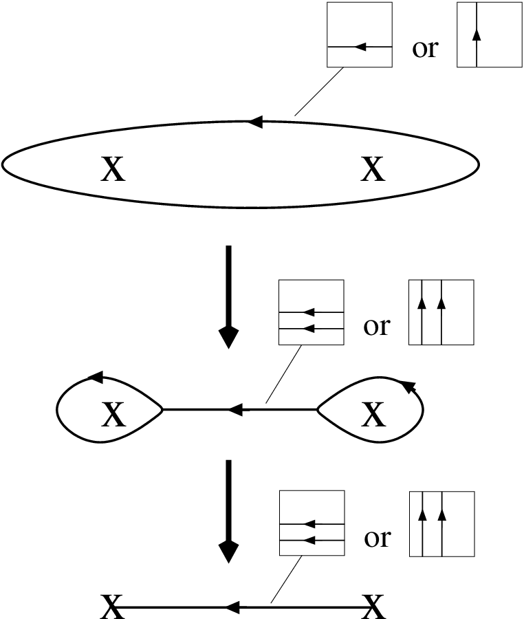
Keeping the construction in the case of a complex one-dimensional base in mind, we can repeat the construction done for the D-brane: we take a disc ending on the O-plane in the base and one of the two fibres in Figure 4.3 to construct a 3-cycle. Just as in the D-brane case, the size of this cycle will describe the recombination process of two intersecting O-planes.
4.2 F-Theory models at the orientifold point
In the following, we discuss F-theory compactifications on elliptic threefolds that can be constructed as orientifolds. In particular, we demand that all D-branes coincide with the O-plane in this section. We are going to describe these models from several perspectives, summarized in Figure 4.4.
4.2.1 The type IIB perspective
Let us start with the well-known type IIB perspective. Besides the various form-fields, the moduli space of type IIB on contains the geometrical moduli space of and the complexified string coupling, also known as the axiodilaton (see e.g. [91]). The geometric moduli can be elegantly described as the rotations of a three-plane of positive norm inside . The three positive-norm vectors that span this three-plane can then be used to construct the Kähler form and the holomorphic two-form . As is common for Calabi-Yau threefolds, the geometric moduli of can then be mapped to Kähler and complex structure deformations.
Apart from the inner parity of the various degrees of freedom coming from the involution of the world-sheet, orientifolding includes an involution of space-time. Furthermore, this involution has to map the holomorphic two-form to minus itself, so that the quotient space is not Calabi-Yau. Involutions of this kind are known as non-symplectic in the mathematics literature and have been classified by Nikulin [131]. We have summarized the main results in Appendix A.6. The classification of non-symplectic involutions of implies that is rational, so that it is a del Pezzo surface , a Hirzebruch surface , or a blow-up of a Hirzebruch surface. For a short review of rational surfaces see Appendix A.5.
Under the action of , the cohomology groups of decompose into eigenspaces:
| (4.6) |
The geometric moduli of this orientifold model were discussed in detail in [142]. The complex structure deformations that are compatible with are in one-to-one correspondence with elements of . As the Kähler form of is even under , compatible Kähler deformations can be parameterized by . Since is a non-symplectic involution, we have .
The fixed point locus of is the orientifold plane . It is given by the vanishing locus of a section of , where denotes the canonical bundle33 3 For a divisor we denote the corresponding line bundle by . of the base space [100]. In other words, the O-plane is equivalent to as a divisor. This is necessary to ensure that the double cover is a Calabi-Yau space. To cancel the D7-brane charge, the homology class of all the D-branes has to equal four times the homology class of the O-plane. In this section we choose to align four D-branes with the O-plane. The only geometric deformations of this configuration are hence given by the Kähler deformations of the base and the deformations of the O-plane. These must be equivalent to the deformations of compatible with the orientifolding.
Let us illustrate this in the simple example of . The sections of are given by homogeneous polynomials of degree 6. We can count the degrees of freedom that correspond to deformations of this polynomial: there are 28 independent monomials and hence 28 complex coefficients. One of these can be set to unity by an overall rescaling. In addition, the embedding of in is only defined up to automorphisms of . This automorphism group is complex 8-dimensional (see Appendix A.4.5), eliminating degrees of freedom. We thus end up with complex degrees of freedom. As , we find that , giving the right number of degrees of freedom. We have collected some more examples in Table 4.1 at the end of the present section.
4.2.2 Deformations of the O-plane
Deformations of a Riemannian surface, such as the O-plane , are given by holomorphic sections of its normal bundle . The dimension of the space of holomorphic sections of is commonly denoted by .
A Riemannian surface, such as the O-plane, has complex structure deformations. Let us explain why this is also the number of deformations in the embedding. From the adjunction formula we have .44 4 Here and in the following the restriction of to is implicit. As is linearly equivalent to , we have and thus find . Serre duality then tells us that
| (4.7) |
in other words we find
| (4.8) |
For later convenience, we show how to derive (4.8) using the Riemann-Roch-Theorem [118]
| (4.9) |
where is the canonical divisor of and the genus of . The degree of a line bundle is the number of zeros of a generic section of . If it follows that . In this case
| (4.10) |
Since a section of the normal bundle is nothing but a deformation of the Riemannian surface, is just the self-intersection number of . As is linearly equivalent to , we find that its self-intersections number is . Furthermore, we find from the Euler characteristic of to be . Hence we obtain
| (4.11) |
Thus the requirement for Eq. (4.10) is satisfied and we find (4.8).
So far, we have neglected the fact that some deformations of the O-plane are equivalent to applying an automorphism of the base and as such do not represent valid complex degrees of freedom. Thus the number of deformations of the O-plane, , is given by
| (4.12) |
where denotes the Lie-algebra of . In the case of a toric variety, this quantity can be found by the procedure explained in Appendix A.4.5.
4.2.3 F-theory perspective
Having discussed the moduli from the type IIB perspective, we now turn to the F-theory description of the same situation. Since we have taken all D-branes to be aligned with the O-plane, the axiodilaton is constant along . The corresponding F-theory description thus must be such that the complex structure of the elliptic fibre is constant. Before orientifolding, there are no monodromies and the F-theory threefold is simply the product . The orientifolding introduces a monodromy that acts as an involution on the fibre . It occurs upon encircling the O-plane locus. We can describe this situation by lifting the involution to an involution on by defining
| (4.13) |
where and and . Modding out yields the F-theory compactification on .
The homology groups of are
since . Keeping the cycles even under yields the homology of :
| (4.14) |
F-theory on emerges from M-theory on the same manifold in the limit of vanishing fibre size. The geometric moduli of M-theory on are deformations of that respect the action. Hence the Kähler and complex structure deformations of are linked to even cycles of . The Kähler moduli of and the volume of the elliptic fibre become the Kähler moduli of . As the fibre size tends to zero in the F-theory limit, it does not give rise to a physical modulus in F-theory, so that we find the same number of Kähler moduli as for the -orientifold .
The 3-cycles of originate from the odd 2-cycles of . The number of complex structure moduli, , of a Calabi-Yau space is given by the number [119]. If we choose a symplectic basis , the complex structure moduli space is locally parameterized by the independent periods:
| (4.15) |
where is the holomorphic 3-form. In the present case, we only consider complex structure deformations that do not destroy the structure (by resolving the orbifold singularities, for instance). We can think of this restriction as fixing a number of periods. The relation between complex structure deformations and , thus holds for an orbifold like as well.
In the present case we find that
| (4.16) |
As the holomorphic two-form of and its complex conjugate are always odd for the involutions considered we have , so that we find
| (4.17) |
In F-theory, the present situation is described by an elliptic threefold in which there is a singularity along a curve that is equivalent to . This curve is the location of the O-plane. The complex structure deformations of the threefold that preserve the singularity structure correspond to deformations of the O-plane and the value of the axiodilaton. This is expressed in (4.17): the number of complex structure deformations equals the number of deformations of the O-plane, , plus one. This fits nicely with the aforementioned result that deformations of the double cover compatible with the orientifold involution originate from cycles of that are odd under the orientifold involution.
There is a subtle point worth mentioning here. In the present case, has four singularities along the location of the O-plane. The manifold constructed from the Weierstrass model that corresponds to the orientifold has however a singularity over the location of the O-plane. Even though for both the fibre torus undergoes the same monodromies [145], they give rise to different physics for compactifications of M-theory. However, in the F-theory limit both manifolds coincide, as they are connected by blow-ups and blow-downs of the singular fibres, leading to the same type IIB model. See Section 3.4 for a discussion of this and related issues.
4.2.4 3-cycles at the orientifold point
In the following, we will discuss how the 3-cycles of emerge from the topology of the O-plane. Let us first return to the example of . In this case the O-plane locus has deformations, so that we expect the corresponding threefold to have complex structure moduli yielding independent 3-cycles.
The local construction of F-theory 3-cycles from the O-plane topology, presented in Section 4.1.2, suggests that we obtain two F-theory cycles for each 1-cycle of the O-plane . Since , where is the genus of , we expect F-theory 3-cycles. As mentioned before, is given by a defining polynomial of degree 6 in the case, yielding a curve of genus . We thus obtain 40 cycles in instead of 42. However, from the global point of view there is exactly one other cycle that could be lifted to a F-theory 3-cycle, namely the cycle corresponding to the hyperplane divisor of . Naively, we can add a leg with two possible orientations in the fibre to so that the lift yields two extra cycles. Including these, we get the right number of 42 cycles. We have collected some more examples in Table 4.1.
There is one potential difficulty to this construction. The hyperplane divisor will generically intersect the O-plane . Since the fibre degenerates on it is not a priori clear how to lift properly. As it will become clear later on, can indeed be lifted to an F-theory cycle but for now this remains a conjecture motivated by the counting.
It is now natural to conjecture that for any base space , the number of non-degenerate cycles in is given by
| (4.18) |
The Lefschetz fixed point theorem [118] allows us to relate the topology of the O-plane to the topology of in the general case. For a surface it reads
| (4.19) |
From this is follows directly that
| (4.20) |
On the other hand, we know that the fixed point locus is given by the disjoint union of a curve of genus and spheres [131], see also Appendix A.6. Thus we have
| (4.21) |
which yields
| (4.22) |
This equation can also be derived directly using (A.111). For the cases in which the O-plane is given by a single smooth complex surface we have , so that (4.18) indeed holds. Note that this is the case in the example of discussed before.
| surface | ||||||
|---|---|---|---|---|---|---|
| 10 | 9 | 8 | 7 | 9 | 9 | |
| 1 | 2 | 3 | 4 | 2 | 2 | |
| 19 | 18 | 17 | 16 | 18 | 17 | |
| Def() | 19 | 18 | 17 | 16 | 18 | 17 |
| 42 | 40 | 38 | 36 | 40 | 38 | |
| 42 | 40 | 38 | 36 | 40 | 40 |
The results for different surfaces are given in Table 4.1. It is interesting to note that in the case of the degrees of freedom in the type IIB picture do not fit the number of complex structure moduli in the F-theory picture. Indeed, in this case one can show that there is one complex structure deformation of the Calabi-Yau threefold which is not realized as a polynomial deformation of the Weierstrass model (see e.g. [120] for a discussion of this phenomenon in the physics literature).
It is nice to see that (4.22) is invariant under blow-ups of the base: As
| (4.23) |
we deduce the Euler characteristic of to be
| (4.24) |
Now consider the blow-up at a generic point . This means we add an exceptional divisor so that . The behavior of the anticanonical divisor under blow-ups is [118]
| (4.25) |
The exceptional divisor can always be chosen to satisfy [146]
| (4.26) |
In particular, this implies . It is now straight forward to determine the Euler characteristic of :
| (4.27) |
Since the Euler characteristic is given by the relation , (4.27) implies that under blow-ups of at generic points. We thus need to show that under blow-ups of the base. As is fixed and the blow-up increases by one, must decrease accordingly. Hence we find , so that (4.22) remains valid.
Formula (4.22) can be given a further interpretation in terms of the double cover . Let us start with the case and consider a 1-cycle of the O-plane. This 1-cycle is trivial inside the base. Thus, there exists a real disk in the base whose boundary coincides with this 1-cycle. If we now go to the double cover, we end up with two disks that are glued together at their boundary, which is located at the 1-cycle of the O-plane. This gives rise to a two-sphere on which is a non-trivial 2-cycle since the corresponding O-plane 1-cycle was non-trivial. Clearly, this 2-cycle is odd under the involution on since the involution changes the orientation of the 2-cycle. When we add the fibre, each combination of this 2-cycle with a 1-cycle in the fibre gives rise to a 3-cycle in the threefold. Hence, we get twice as many 3-cycles on the threefold as there are 1-cycles on the O-plane, i.e. many. This construction is a further motivation for the cycles that were constructed locally in Section 4.1.2. If one builds the double cover of branched along the vanishing locus of an equation of the form (4.2) one finds the space blown up at the origin. The exceptional cycle of this blow-up is an odd 2-cycle under the orientifold projection. Its image under the orientifold projection yields precisely the base part of the 3-cycle that controls the O-plane motion in F-theory.
Let us now turn to the contribution coming from and consider a 2-cycle of . Recall that . Since we assumed , we have , cf. Appendix A.6, and every basis 2-cycle of can be understood as the sum of two (maybe intersecting) basis 2-cycles of that are exchanged by the involution. Then, the difference of these basis 2-cycles gives an element in , which can be combined on with one of the fibre 1-cycles to build an even 3-cycle that descends to the threefold. By this we obtain two 3-cycles of the threefold for each 2-cycle in B. This explains the second contribution in (4.18). For , we have .
Now let us discuss the case of nonzero . This means that we now additionally have non-trivial rigid two-spheres in that are part of the fix point locus, i.e. which are filled out by the O-plane. Let us consider one of them. Clearly, this cycle has only one pre-image in , which is left fixed by and thus even under the involution map. Furthermore, we can write (A.111) as
| (4.28) |
so that it follows that there must be a second even cycle for any fixed . All of these cycles do not lead to any 3-cycle on the threefold and do not contribute to (4.18). As the quantities and are actually not independent, but related by (A.111), we find (4.22).
Note that from this discussion we see that we can decompose the second cohomology class of into three parts, corresponding to
- •
spheres consisting of fix points plus further cycles, all of them being even under the involution,
- •
pairs of cycles which are interchanged
- •
spheres which are invariant up to an orientation reversal.
The fact that these cycles give the correct number of 2-cycles of , i.e.
| (4.29) |
follows directly from (A.111).
4.3 D7-branes without obstructions
4.3.1 Pulling a single D-brane off the orientifold plane
In this section we now want to leave the orientifold point by moving one D-brane off the O-plane. The most general form of the hypersurface which is the position of the D-branes is given by [79]
| (4.30) |
where and are sections in and , respectively. We will call a D7-brane described by an equation of the form above a generic allowed D7-brane. Note that the equation describes the position of the O-plane . At the orientifold point, the O-plane coincides with four D-branes, so that and and Eq. (4.30) reads
| (4.31) |
We can now vary the sections and in order to deform the D-branes. Choosing and , where is a section in , then yields
| (4.32) |
The surface consists of four components: three D-branes still coincide with while one is deformed and thus separated from the O-plane. The deformation is given by the generic section which is of the same degree as . This fits nicely with the fact that infinitesimal deformations of a surface correspond to sections in the normal bundle of .
Let us first return to the example of . We can count the number of deformations of the single D-brane that is moved off the O-plane by counting the monomials of and subtracting the one complex degree of freedom of overall rescaling. Note that fixing the O-plane in generically breaks the automorphism group of completely and thus its dimension does not reduce the number of degrees of freedom. In the present case, will be a homogeneous polynomial of degree 6 yielding complex degrees of freedom.
The number of deformations can also be obtained by analysing sections in the normal bundle of the D-brane. As the D-brane we are considering is linearly equivalent to , the analysis of the previous section leading to Eq. (4.8) applies. As the genus of the D7-brane is given by in the case of , we can immediately confirm that the number of deformations is given by . Following an argument similar to the one presented in Section 4.2.3 we thus expect to find 2-cycles that govern the displacement of a single D-brane that is equivalent to from the O-plane in . It is clear that a similar computation can be performed for other base spaces.
3-cycles between O-plane and D-brane
We now construct the 3-cycles that describe the process of moving a single D-brane off the O-plane. Let us first discuss the analogue of these cycles for F-theory compactified on , where O-plane and D-brane are points rather than complex lines. We can link the two by a path that begins at the D-brane, encircles the O-plane and then ends at the same D-brane. To construct a 2-cycle, we add the horizontal fibre to every point of this curve, see Figure 4.5.

The existence of this cycle can also be demonstrated by the following argument: two D-branes in the vicinity of an O-plane can be connected by a cycle in two ways: the cycle can pass the O-plane on one side or the other [74]. We can find a cycle that connects just one of the two D-branes to the O-plane by forming the sum (or difference) of these two cycles. The resulting cycle has self-intersection number and can be deformed to any of the two representatives discussed in Figure 4.5.
Coming back to F-theory compactified on an elliptically fibred Calabi-Yau threefold, we can generalize this construction as follows. We choose a 1-cycle of the D-brane and a representative . Since we are considering the case in which the D-brane has the same topology as the O-plane, we can find a corresponding cycle and representative on the O-plane that coincides with when D-brane and O-plane are on top of each other. Now we apply the above construction to every point . In other words, we fiber with the 2-cycles of Figure 4.5. In this way we obtain 3-cycles that measures the distance between the D-brane and the O-plane.
3-cycles from intersections between D-brane and O-plane
Another type of cycle can be constructed as follows. Consider two intersection points and of the D-brane with the O-plane (see Figure 4.6). Since is connected, we can find a loop that surrounds both intersection points. This immediately implies that can only be contracted if coincides with . We know from Section 4.1 that the disc in B the boundary of which is can be lifted to a 3-cycle in the threefold . Indeed, we again fiber the 1-cycle of the torus that degenerates at the D-brane over the disk. This 3-cycle cannot be contracted due to the presence of the O-plane. The involution on the fibre which is part of the monodromy of the O-plane prevents the disk from passing through the O-plane position – the fibre will simply be ill-defined if the disk intersects the O-plane. Clearly, this 3-cycle has again the topology of a three-sphere and its volume is proportional to the distance between the intersection points with the O-plane.

We can understand this 3-cycle also in another way. We can fiber the 2-cycle of Figure 4.5 over the line on the D-brane that connects the two intersection points with the O-plane.
Let us now count the number of independent cycles that can be constructed in this way. Suppose there are intersection points on . Let be a disc such that is a loop on which surrounds the intersection points and . The boundaries are elements of the first homology group of the D-brane with the O-plane cut out, . Note that and will generically intersect only in (two) points that are located on the D-brane world volume since the D-brane and the cycles have codimension two (cf. Figure 4.7). This yields such loops55 5 We identify with . and each loop gives a relative 2-cycle . The cycles we construct in this way are not linearly independent. We can construct the union
| (4.33) |
The boundary of the relative 2-cycle surrounds all intersection points on except for and . Since D is compact, this is equivalent to saying that surrounds just and . Thus, is relatively homologous to and hence is not independent of the others. In the previous argument we just used half of the , namely those where is odd. We showed that one cycle can be expressed as a linear combination of the others. The same argument goes through for the complementary subset of where is even. Having constructed 2-cycles , we are now left with independent F-theory 3-cycles. This is illustrated in Figure 4.7.

Putting everything together, the number of 3-cycles we obtain by the constructions presented is . As discussed before, the intersection number of D-brane and O-plane is nothing but the self-intersection number of . From Eq. (4.11) we thus know that . Adding the cycles coming from the 1-cycles of the D-brane and the cycles coming from the intersections with the O-plane, we arrive at the total number of . These cycles determine the infinitesimal separation of the D-brane from the O-plane. This fits exactly with the number of general deformations of Riemann surfaces obtained before. We conclude that the union of both kinds of 3-cycles parameterize the location of the D-brane.
Coming back to the example of , we find that and , so that we can construct cycles. This precisely fits the expectation expressed at the beginning of this section.
4.3.2 More general configurations
We now want to generalized the discussion to the case of multiple D-branes separated from the O-plane. When we move multiple branes off the O-plane and let them recombine, we can no longer describe the resulting D-brane locus in terms of sections in the normal bundle of the O-plane. Furthermore the worldvolume of the D-brane will in general be no longer be a generic hypersurface as it is forced to have double intersections with the O-plane [74, 41]. Namely, is given by Eq. (4.30). However, the D-brane curve will still be a generic hypersurface if we consider one of the following configurations:
- i)
We leave one D-brane on the O-plane. This corresponds to choosing , where is a section in . This yields
(4.34) Since is generic, is. Note that is a section in and therefore describes three recombined D-branes generically not coinciding with the O-plane. The resulting D-brane locus is appropriately described by a generic hypersurface in , the zero locus of , as required. The polynomial shows that one D-branes still sits on the O-plane.
- ii)
We move all D-branes in stacks of two. This case corresponds to the choice so that the D-brane is described by and hence a generic section in .
In this section we analyse configurations in which the D-brane degrees of freedom are associated to the deformation moduli of a generic hypersurface of lower degree. For the whole analysis, we completely fix the O-plane and focus on the D-brane degrees of freedom.
We start again with the example where is the base space and analyse the general case afterwards. Assume that in addition to the O-plane we have a D-brane that is linearly equivalent to , i.e. whose locus in is described by the vanishing of a homogeneous polynomial of degree . Due to the D7 tadpole cancellation condition, this means that D-branes still coincide with the O-plane. As the presence of the O-plane generically breaks the whole automorphism group of , this D7-brane has
| (4.35) |
complex degrees of freedom.
In the last section we found that a D7-brane that is equivalent to has complex degrees of freedom and gives rise to 3-cycles in the threefold. In the remainder of this section, we show that this statement holds for any D7-brane that is equivalent to for any . The reader primarily interested in results may wish to skip the rest of this section and continue with Section 4.4.
Let us now try to find an analog of Eq. (4.35) for an arbitrary base space . We will formulate all relevant quantities in terms of the self-intersection of the anti-canonical divisor of the base, . For any F-theory model, the worldvolume of the O-plane is equivalent to the divisor . We consider the situation with recombined D-branes and D-branes coinciding with the O-plane. In order to apply the Riemann-Roch Theorem, cf. Eq. (4.10), we need to know the degree of the canonical divisor of , denoted by . It is given by
| (4.36) |
The Euler characteristic of is
| (4.37) |
so that the genus is given by
| (4.38) |
Thus we find the degree of to be
| (4.39) |
The self-intersection number of is , so that the condition is satisfied. Hence we can use Eq. (4.10) to find the number of valid deformations:
| (4.40) | ||||
In the last line we have used that the number of intersections between the D-brane and the O-plane is
| (4.41) |
We thus expect to find 3-cycles that govern the deformation of the D-brane locus.
From the relation derived in the last paragraph it is clear how the 3-cycles that control the motion of a D-brane arise: On the one hand, we can build a 3-cycle from every 1-cycle of the D-brane, using the construction given in Section 4.1.1. On the other hand, we can build cycles that measure the distance between intersections of the D-brane with the O-plane, as discussed in Section 4.3.1.
This can also be understood from the perspective of the double cover as we now explain qualitatively. It is known that for a smooth D-brane in the double cover, i.e. one that does not have double intersections with the O-plane, the deformations are given by 1-cycles of the D-brane that are odd under the involution [40]. As this is the situation discussed in this section, we should be able to link the 3-cycles we have constructed to odd 1-cycles of the D-brane in the double cover.
A 1-cycle of a D-brane in that has been moved off the O-plane generically does not intersect the O-plane. Furthermore, we can always deform the 1-cycle such that its winding number is zero with respect to the O-plane. Therefore, this 1-cycle has two pre-images in the double cover which are interchanged by the involution. The sum of both is even under the involution and therefore descends to the 1-cycle of we started with. The difference of both, however, is odd under the projection and should refer to a deformation of the D-brane. This suggests a fact already discussed: 1-cycles of are related to 3-cycles of the Calabi-Yau threefold. Furthermore, we can consider a line on connecting two intersection points of with the O-plane and go to the double cover . This line then becomes two lines joined at their end points, i.e. a non-trivial closed 1-cycle on the double cover D-brane that is odd under the involution. Thus, there should be a second kind of 3-cycles which are closely related to the intersections of the D-brane with the O-plane, supporting our claim that we can construct 3-cycles from intersections between the D-brane and the O-plane.
As the intersections between O-plane and D-brane are points on a complex curve, one naively expects each intersection point to correspond to a complex degree of freedom. From the relation between moduli and 3-cycles it follows that there should roughly be 3-cycles that stem from intersection points between D-brane and O-plane. This is, however, not the case, as we only found half of that. Thus there seems to be some mismatch here. The solution to this puzzle is that fixing the periods of the one-cycles of the D-brane leaves only few degrees of freedom for the intersection points with the O-plane to vary. Hence the displacement of the intersection points is governed not only by the 3-cycles that are attached to intersection points but also through the 3-cycles that stem from the 1-cycles of the D-brane.
Compared to Section 4.3.1, our cycle analysis is complicated by the fact that the O-plane can in principle pierce a disc that ends on a 1-cycle.66 6 As we will discuss in more detail later, this is ultimately related to the structure of branch cuts on the D-brane when building the double cover. The monodromy of the O-plane then prevents the construction of a 3-cycle as its fibre part is transformed to a different cycle upon encircling the O-plane locus. To tell if we can find a disc that ends on a given loop on the D-brane and does not intersect the O-plane, we need to check that the winding number of this loop around the O-plane vanishes. We can define the winding number on the first homology of the D7-brane with the intersection points with the O-plane cut out, , and then project to the subspace of zero winding number. Since has the dimension and there are elements of that have a non-zero winding number, this projection leads to a subspace of dimension , i.e. we find independent cycles we can use to construct non-trivial 3-cycles of the elliptic fibration. This reproduces the result that is expected from an analysis of the degrees of freedom of a D-brane.
Let us again come back to the example of . In this case one easily finds the numbers and , so that
| (4.42) |
which exactly matches the number of degrees of freedom, as given by (4.35).
Note that we can use the reasoning presented in this section also for the situation discussed at the beginning of this section, in which a single D-brane is moved off the O-plane. Although we used different 3-cycles in both cases, the results agree as expected. The two sets of cycles just give a different basis of the third homology group of the threefold.
We can also give an inductive construction of 3-cycles in terms of (relative) 1-cycles as long as all D-branes are described by completely generic hypersurfaces. We start with the case in which the D-brane locus and the O-plane locus coincide. These cycles were discussed at length in Section 4.2. New cycles appear when the first D-brane is moved away from the O-plane, namely the cycles given in Section 4.3.1. We used in this analysis that the D-brane is given by a section in the normal bundle of the O-plane.
We can now independently move two D-branes off the O-plane, both given by sections in the normal bundle of . Additionally to the cycles for described in Section 4.1.1, there are intersections between the two D-branes. Thus, the D-brane locus is a nodal Riemann surface with nodes, where denotes the number of intersection points of the two D-branes. By generic deformations of these singular intersection points, the D-branes recombine at these nodes as described in Section 4.1.1, yielding a smooth Riemann surface . Note that the genus of is identical to the arithmetic genus of . For the arithmetic genus the following identity holds [143]
| (4.43) |
where is the nodal Riemann surface with nodes and irreducible components which have the geometric genus , respectively. In our case of interest, Eq. (4.43) reduces to
| (4.44) |
where denotes the single D-brane. Using Eq. (4.40) we can immediately give an expression for the number of independent deformations of :
| (4.45) | |||||
Here denotes the intersection number between and and we used that . The first term in the last line in Eq. (4.45) are the degrees of freedom obtained by moving the D-branes independently. The second part, namely , gives the number of recombination parameters. Each intersection point gives exactly two cycles. In fact, these are locally the recombination cycles obtained in Section 4.1.1. In the same way we can discuss the case of three D-branes moved off the O-plane.
4.4 D7-branes with obstructions
4.4.1 D-brane obstructions
In the weak coupling limit the D7-brane locus is not given by the zeros of a generic polynomial, but by the zeros of a polynomial of the form
| (4.46) |
We refer to D7-branes that are described by an equation of this form as generic allowed D7-branes. As has recently been discussed [74, 41], this form forces the D7-brane to have double intersections with the O7-plane. From the perspective of F-theory this means that the D7-brane forms a parabola touching the O-plane in the origin, see Figure 4.8.
Let us try to understand this configuration from the double cover perspective. Consider two D-branes at and the involution , which fixes the O-plane at . After modding out the involution, our space looks locally like the upper half plane. In order to make contact with the F-theory picture, we introduce a new coordinate and find that this situation is described by an O-plane at and a D-brane at . Note that a single D7-O7 intersection in F-theory (which does not occur in the weak coupling limit), corresponds to a single D7-brane that is mapped onto itself by the orientifold projection. This configuration, where the D-brane sits e.g. at is allowed in the presence of a second D-brane that coincides with the O-plane.
In [74] it was observed that the difference between the degrees of freedom of a generic allowed D7-brane and the degrees of freedom of a generic hypersurface of the same degree is given by half the number of intersections between the D7-brane and the O7-plane77 7 Here we of course count the topological intersections between two generic surfaces that are homologous to the D7-brane and the O7-plane.. We checked this explicitly only for base spaces and . Here we extend this analysis to all possible base spaces. We use the fact that a generic hypersurface that is linearly equivalent to has
| (4.47) |
deformations. To simplify equations we again use as a shorthand for . As in the last section we keep the O-plane fixed so that the automorphism group of the base is completely broken. As the number of double intersections is given by , the double intersections lead to constraints, so that we expect the number of deformations encoded in Eq. (4.30) to be
| (4.48) |
The degrees of freedom in the expression (4.30) are given by the number of monomials in and , minus an overall rescaling and the redundancy that corresponds to shifting by , being a polynomial of appropriate degree. To compute the number of monomials, we note that we can take the polynomials , and to define hypersurfaces on their own and compute the number of their deformations using Eq. (4.47). The number of monomials is then given by the number of deformation plus one. For a D7-brane that is equivalent to , , and are sections of , and , respectively. Thus the degrees of freedom in Eq. (4.30) are given in this case by
| (4.49) | ||||
which coincides with (4.48).
For a generic hypersurface one can actually show that in the double cover its deformation space is isomorphic to , where is the corresponding preimage of in the double cover [40]:
| (4.50) | ||||
where the first of the above equalities follows from the Riemann-Hurwitz theorem [118]. We want to stress that the above statement is not true any more for a generic allowed brane and its double cover . More precisely, we see from (4.49) that the number of degrees of freedom is exactly . A comparison with the computation in (4.50) suggests that the cycles in which are related to the double intersections do not give rise to deformations of .
Let us now perform an analogous computation for the generic allowed brane and its double cover to confirm this observation. As we already discussed in Figure 4.8 and below (4.46), is a smooth brane apart from its self-intersections (which occur at every intersection point with the O-plane). Removing these singular points from , we obtain a smooth Riemann surface with punctures on which the orbifold projection acts freely. Subsequently, we compactify this punctured Riemann surface in the obvious way, by adding one point per puncture. The result is a smooth compact Riemann surface with free action, which we continue to call by abuse of notation. While this smooth Riemann surface is not realized as a submanifold of the double-cover Calabi-Yau, its projection is still our familiar generically allowed D-brane given as a submanifold of the base . By standard arguments [40], its allowed deformations correspond to -odd sections of the canonical bundle of , which is understood as a smooth Riemann surface as explained above. Thus, repeating the calculation of (4.50), the number of deformations is given by
| (4.51) |
where we have again used the Riemann-Hurwitz theorem, but now for a freely acting involution. This agrees with our previous results. The advantage of this new derivation is that we are now able to specify which bundle over encodes these deformations. Indeed, while the even sections of correspond to sections of , the odd sections of can be understood as sections of a ‘twisted’ canonical bundle over . The latter is is defined as the projection of , where the action on is supplemented by a ‘’ action on the fibre. Locally, in a small neighbourhood of an intersection point with the O-plane, this is still the canonical bundle of , in agreement with the discussion of [61, 62, 149].
4.4.2 Recombination for double intersection points
Now we want to understand the number of 3-cycles from the threefold perspective and explain why the number of 3-cycles is reduced by when compared with our results in Section 4.3. As mentioned above, we need to understand the winding numbers of the D-brane 1-cycles relative to the O-plane. First we discuss this locally for a single 1-cycle and then in Section 4.4.3 analyze the global situation.
Let us again consider the recombination of two intersecting D-branes, cf. Section 4.1.1, but now in the presence of the O-plane at the intersection point. Furthermore, we assume that we have already moved the fourth D-brane off the O-plane such that we describe the D-branes by Eq. (4.30). If we set in the local model
| (4.52) | ||||
we have the situation of an O-plane at and a D-brane given at
| (4.53) |
For , it parameterizes the situation of two D-branes at and an O-plane at , all of them intersecting at the origin, as shown in the left picture in Figure 4.9. If we now give a non-zero value, we get to the recombined situation to the right in Figure 4.9.

Here the diameter of the throat connecting the two D-branes is given by . After recombination, the O-plane touches the D-brane tangentially at , see Fig. 4.10.

With help of Eq. (4.53), we can picture the D-brane as the -plane with a branch cut between the two branch points at and , as shown in Figure 4.11.

The intersection with the O-plane is also given by , and therefore, the D-brane 1-cycle encircles the O-plane intersection exactly once. However, since the O-plane is just a plane parameterized by , any loop on the D-brane world-volume encircling encircles, when understood as a curve in , the O-plane exactly once, too. Thus, the D-brane 1-cycle has a winding number of one relative to the O-plane.
Since the D-brane 1-cycle wraps the O-plane exactly once, we cannot build a 3-cycle out of it as done in Section 4.1.1. Because of the involution of the O-plane the fibre would simply be ill-defined. From the double cover perspective, it is clear that the 3-cycle construction fails for a D-brane 1-cycle with an odd wrapping number: In the double cover, the lift of this 1-cycle is not closed and does not define a D-brane 1-cycle in the double cover.
4.4.3 Threefold cycles, obstructions and the intersection matrix
In this section we outline how threefold three-cycles arise from the topology of a generic allowed D-brane, analogously to Section 4.3.1. We do not provide a rigorous proof but rather sketch the construction of threefold 3-cycles from the 1-cycles of a generic allowed D-brane in the presence of a ‘naked’ O-plane. Using (4.40) we can express the number of degrees of freedom of a generic allowed brane in terms of its genus:
| (4.54) |
We thus expect that we can construct 3-cycles. All intersections of the D-brane with the O-plane are double intersections, which makes it impossible to construct cycles in the spirit of Section 4.3.1. However, we still can build 3-cycles related to the D-brane 1-cycles, as we explain now. For this, we first choose a symplectic basis for the 1-cycles of the D-brane and then discuss how the basis 1-cycles lead to 3-cycles in the threefold, depending on the wrapping number of these 1-cycles with respect to the O-plane. We illustrate the curves on the D-brane that lead to 3-cycles in Fig. 4.12.

Note that Fig. 4.12 represents a local picture of the D-brane, ignoring the topology of and of the O-plane.
Consider a symplectic pair of D-brane 1-cycles. First assume that both 1-cycles have zero wrapping number with respect to the O-plane. If this occurs, we can construct a 3-cycle over each of them as explained in Section 4.1.1, giving a symplectic pair of 3-cycles which has no intersection with any of the other 3-cycles. An example of such a symplectic pair is given by C and D in Fig. 4.12.
Next consider a symplectic pair of 1-cycles where one of the 1-cycles has wrapping number one while the paired cycle has still wrapping number zero. An example of such a pair is given by C1 and D1 in Fig. 4.12, where D1 has wrapping number one and C1 has wrapping number zero. If we try to use the same technique as in Section 4.1.1 and fibre the usual 1-cycle over a disc ending on D1, we cannot close this 3-cycle since the monodromy of the O-plane inverts the orientation of the fibre 1-cycle. One might have the idea to use a loop corresponding to 2D1, which surrounds the O-plane twice. Since the orientation of the fibre 1-cycle is inverted twice, the corresponding 3-cycle is closed. However, this 3-cycle must be trivial since it is by construction symmetric under orientation reversal, i.e. the 3-cycle is equivalent to minus itself.
This result has several consequences. First of all, we see that if we have a symplectic pair of 1-cycles where both have an even wrapping number, we can always add 2D1 such that the wrapping numbers are zero and apply the construction method of Section 4.1.1 to find two 3-cycles. This should be seen in contrast to Section 4.3, where one had to restrict to the D-brane 1-cycles that have zero wrapping number and thereby reduced the number of appropriate 1-cycles by one. Secondly, the construction of 3-cycles from cycles with odd wrapping number must be modified. Note that if both 1-cycles of a symplectic pair have an odd wrapping number, we can replace one of them by the sum of both, leading to a symplectic pair of 1-cycles where only one wrapping number is odd. Thus, the remaining case is that exactly one of the two D-brane 1-cycles has an odd wrapping number.88 8 The number of such symplectic pairs is actually , as we explain now. If we consider Eq. (4.30) with , this corresponds to two D-branes at which then can be recombined at each of the intersection points. With the result of Section 4.4.2 we conclude that there are D-brane 1-cycles with odd wrapping number. These 1-cycles correspond to the double intersections of the D-brane with the O-plane.
As discussed above, over a D-brane 1-cycle with odd wrapping number no 3-cycle can be defined due to the involution that is part of the O-plane monodromy. However, we can use the sum of two such 1-cycles which is represented by a curve encircling two of the double intersection points with the O-plane. Examples of such curves are denoted in Fig. 4.12 by and . Note that since 3-cycles constructed out 2D1, 2D2 oder 2D3 are trivial, the third combination does not lead to any independent 3-cycle but to the one constructed out of . Thus, this construction gives us one 3-cycle less than there are D-brane 1-cycles with odd wrapping number.
Now we turn to the 1-cycles that are dual to those with odd wrapping number, represented by C1, C2 and C3 in Fig. 4.12. Since these 1-cycles have even wrapping number we can construct 3-cycles out of them. However, there is a linear dependence between them, as we show now. Consider the curves B1 and B2 in Fig. 4.12. They both lead to non-trivial 3-cycles due to the intersection points of the D-brane with the O-plane. Since the involution of the O-plane inverts the orientation of the fibre 1-cycles, the 3-cycle comes back to minus itself when once encircling the O-plane. More precisely, if we denote the corresponding 3-cycles by and , due to the monodromy of the O-plane there is
| (4.55) |
leading to
| (4.56) |
On a general D-brane, the linear dependence analogously reads
| (4.57) |
where the sum runs over all 3-cycles which are coming from D-brane 1-cycles dual to those with odd wrapping number. Thus, we find that the total number of 3-cycles coming from the D-brane sector is two less than the number of 1-cycles of the D-brane, leading to 3-cycles. This coincides with the result we achieved in Section 4.4.1.
Let us now discuss the intersection matrix of the 3-cycles discussed here. As already stated above, the intersection matrix of the 3-cycles that come from 1-cycles with even wrapping number is the standart symplectic one. For the 3-cycles which are constructed out of curves of type A and B, the corresponding 3-cycles and also form a symplectic basis.99 9 Note that the do not intersect each other due to the monodromy of the O-plane. Thus, we find the symplectic basis for the 3-cycles of the threefold that come from the D-brane sector.
Chapter 5 F-theory on fluxed
In this chapter we consider flux stabilization of M/F-theory on . We are able to demonstrate how fluxes stabilize D7 branes or stacks of D7 branes in a completely explicit fashion. This allows us to select a specific desired gauge group by the choice of flux numbers. As explained above, this is the same procedure required for the flux stabilization of non-Abelian gauge symmetries in the (non-perturbative) F-theory context, which has recently attracted significant attention in the context of GUT model building [61, 62, 60, 63, 64]. We therefore expect that straightforward generalizations of our methods will be useful both for more complicated D7 brane models as well as for their non-perturbative F-theory cousins.
Moduli stabilization by fluxes in M-theory on has been studied extensively in the past, especially in relation with the type IIB dual (see, e.g. [58, 158, 59]). In our work we derive the flux potential for the geometric moduli from dimensional reduction. We express it in a form manifestly invariant under the symmetry of the moduli space. In this form, it is immediate to see how the minimization condition is translated into a condition on fluxes and on geometric data of the two ’s. We find all Minkowski minima, both supersymmetric and non-supersymmetric. An analogous explicit search for (supersymmetric) flux vacua has been reported in [150]. Our results are more general since we do not restrict ourselves to attractive surfaces, where a maximal number of integral 2-cycles are holomorphic.11 1 At a technical level, this means that only a discrete set of values are allowed for the various complex structure moduli. There is then also only a very restricted set of fluxes which are suitable for stabilizing such points.
Our analysis of moduli stabilization is also more explicit than the previous works on , since we use a parameterization of D7-brane motion by the size of integral 2-cycles, as derived in Chapter 3. Thus, at least in the weak coupling limit, we have a simple geometric interpretation for every integral basis cycle. Using the choice of flux numbers, this gives us full control over the positions of 4 O7 planes and 16 D7 branes moving on a base (corresponding to type IIB on ).
Our techniques can be used to study the stabilization of all the gauge groups that can be realized by F-theory on . It turns out that tadpole cancellation is very restrictive and allows only very special flux choices.
We begin our analysis in Section 5.1 with a derivation of the flux potential, which closely follows the generic Calabi-Yau derivation of [57, 54, 56]. We emphasize the fact that, due to the hyper-Kähler structure of , its geometric moduli space can be visualized by the motion of a three-plane in the 22-dimensional space of homology classes of 2-cycles. This three-plane is spanned by the real and imaginary parts of the holomorphic 2-form and by the Kähler form. The resulting symmetry of the geometric moduli is manifest in the expression for the scalar potential we arrive at. The three-dimensional theory also has a number of gauge fields, and the flux induces mass terms for some of them, which we derive explicitly. This breaking of gauge symmetries can be understood in the dual type IIB picture as the gauging of some shift symmetry in the flux background.
In Section 5.2 we analyse the minima of the flux potential. To preserve four-dimensional Poincaré invariance, we consider 4-form fluxes that belong to . A flux of this form gives rise to a linear map between the spaces of 2-cycles of the two ’s: integrating the flux on a 2-cycle of one we get a 2-form on the other (which is Poincaré dual to a 2-cycle). Minkowski vacua arise if the flux maps the three-planes determining the metric of the ’s onto each other. We derive the conditions the flux matrix has to satisfy in order for two such planes to exist and to be completely fixed by the choice of fluxes. Furthermore, we clarify the more restrictive conditions under which the plane determined by the flux is consistent with the F-theory limit. In this case, the plane cannot be fixed completely. The unfixed moduli correspond to Wilson lines around the of the type IIB model which decompactifies in the F-theory limit. These degrees of freedom are not part of the moduli space of type IIB compactified to four dimensions, as they characterize the (unphysical) constant background value of one component of the four-dimensional vector fields. In fact, the corresponding propagating degrees of freedom become part of the four-dimensional vector fields (see [139] for a comprehensive analysis of the duality map between the 4d fields of M-theory on and type IIB string theory on ).
The main point of this chapter, the explicit stabilization of D-brane positions, is the subject of Section 5.3. After recalling the parameterization of D7-brane motion in terms of M-theory cycles derived in Chapter 3, we provide explicit examples of flux matrices which fix situations with gauge symmetries , and . In all cases we also fix the complex structure moduli of the lower . The first case corresponds to the orientifold, where 4 D7 branes lie on top of each O7 plane. In the second case, one D7 brane is moved away from an O plane. Finally, in the third case, a stack of two D7 branes is separated from one of the O planes. In these examples almost all the Kähler moduli (which correspond to deformations of the lower and do not affect the positions of the D7 branes) are not stabilized. When one of them is stabilized, a Kähler modulus of the upper is stabilized, too. As mentioned before, this corresponds to some gauge field becoming massive. To clarify this point, we present two examples where one of the D7 branes is fixed at a certain distance from its O plane: In the first example, one further Kähler modulus is fixed, breaking the gauge group. This phenomenon of gauging by fluxes is common in flux compactifications[152, 153, 151, 40]. In the second example, we stabilize the single D7 brane without fixing further Kähler moduli and hence without gauge symmetry breaking. We also provide an example where almost all moduli are fixed. In this case, only the fibre volume of F-theory, the volume moduli of the two s, and three metric moduli of the lower remain undetermined.
Section 5.4 contains a brief discussion of supersymmetry. Generically, we obtain vacua of no-scale type. For specific, non-generic choices of the flux matrix, we find three-dimensional or supersymmetry. To determine the amount of surviving supersymmetry, it suffices to know the eigenvalues of the flux matrix restricted to the two three-planes.
5.1 Flux Potential
In this chapter we compactify M-theory to three dimensions on and analyse the effects of 4-form flux. The main new points of our presentation are the following: We maintain a manifest symmetry of the moduli space of in the calculation of the potential in Section 5.1.2. Furthermore, we explicitly derive the flux-induced masses for the vector fields arising from the 3-form in Section 5.1.3.
5.1.1 M-Theory on
The compactification of M-theory on a generic four-fold is described in detail in[54]. Here we specialize to the case of . To distinguish the two ’s, we write the compactification manifold as . Correspondingly, all quantities related to the second will have a tilde.
The relevant M-theory bosonic action is[154]
| (5.1) | ||||
where is the eleven-dimensional Planck length, , and and are polynomials of degree 4 in the curvature tensor [155, 156]. When we compactify on , we obtain a three-dimensional theory with eight supercharges, i.e. in three dimensions. This can be inferred from the fact that each has holonomy group and correspondingly two invariant spinors.
Let us analyse the geometric moduli. is a hyper-Kähler manifold: its metric is defined by three 2-forms in plus the overall scale. is a 22-dimensional vector space equipped with a natural scalar product,22 2 Throughout this work, we freely identify forms, their cohomology classes, the Poincaré-dual cycles and their homology classes.
| (5.2) |
which has signature , i.e. there are three positive-norm directions. The three vectors defining the metric must have positive norm and be orthogonal to each other. Hence they can be normalized according to . The Kähler form and holomorphic 2-form and can then be given as
| (5.3) |
This definition is not unique: we have an of possible complex structures and associated Kähler forms. Each of them defines the same metric, which is then invariant under the that rotates the ’s.
The motion in moduli space can now be visualized as the motion of the three-plane spanned by the ’s, which is characterized by the deformations of the preserving orthonormality. The corresponding are in the subspace orthogonal to , which is 19-dimensional. Together with the volume, this gives scalars in the moduli space of one . The same parameterization can be used for the second , where the corresponding scalars are and the components of . Altogether one finds scalars from the metric on . Furthermore, since has no harmonic 1-forms, there are no 3d vectors coming from the metric.
5.1.2 The Scalar Potential
We now allow for an expectation value for the field strength of the form
| (5.4) |
where (with ) is an integral basis of . The flux satisfies a (Dirac) quantization condition33 3 The precise quantization condition for a generic fourfold is , where is the first Pontryagin class[157]. Since is even for , the quantization condition becomes simply . : . In the following, we will always denote this type of flux by while the generic 4-form field strength will be .
The flux potential for the moduli is found by reducing the M-theory action. In the presence of fluxes, the solution to the equations of motion is a warped product of a Calabi–Yau fourfold and a three-dimensional non-compact space[54, 59, 33]. In the following, we neglect backreaction and work with the undeformed Calabi–Yau space as the internal manifold. The underlying assumption is that, in analogy to[33], for any zero-energy minimum of the unwarped potential a corresponding zero-energy warped solution will always exist. After Weyl rescaling, the potential is given by[56]
| (5.5) |
where is the Euler number of the compact manifold. For , it is . Given our previous discussion of moduli space, we expect that (5.5) will be invariant under rotations once we express the metric in terms of and .
In the absence of spacetime-filling branes, the cancellation of -brane-charge on the compact manifold requires[54]
| (5.6) |
This allows us to express the second term in (5.5) through the flux. It is convenient to set and to introduce a volume-independent potential by writing . Here is the volume of . Our result now reads
| (5.7) |
with given by (5.4).
On , each can be split into a sum of two vectors, parallel and perpendicular to the 3-plane :
| (5.8) |
Here is the projector on the subspace orthogonal to . The first term, which corresponds to the projection on , has been given in a more explicit form using the orthonormal basis of the plane for later convenience. The two terms of (5.8) represent a selfdual and an anti-selfdual 2-form[57], allowing us to write the Hodge dual of a basis vector as
| (5.9) |
The same applies to .
If we insert (5.4) and (5.8) into the expression (5.7) for and we use the relation (5.9) for the action of the Hodge , we find
| (5.10) | ||||
Since
| (5.11) |
we can write as
| (5.12) | ||||
To write it in a more compact form, we define two natural homomorphisms and by
| (5.13) |
where , and , represent the metrics in the bases , . The operator is the adjoint of , i.e. . The matrix components of these operators are and .
The moduli potential is then given by
| (5.14) |
As expected, it is symmetric under rotation of the ’s and of the ’s44 4 The projectors and are obviously symmetric as they project onto the space orthogonal to all the ’s..
This potential is positive definite since the metrics for and defined in (5.2) are negative definite on the subspace orthogonal to the ’s and the ’s. We note also that the volumes of the two ’s are flat directions parameterizing the degeneracy of the absolute minimum of the potential, in which .
We can also rewrite this potential expressing the projectors through the ’s:
| (5.15) |
This is again manifestly symmetric under rotations.
The Potential in Terms of and
The scalar potential can also be expressed in terms of two superpotentials. For a , it reads [56]
| (5.16) |
Here and and are given by
| (5.17) |
The complex structure moduli are labelled by , while counts the Kähler moduli.
For , we get a similar but not identical form. Note fist that the above potential depends on real moduli. This is the dimension of the metric moduli space of a . But it is not the case for , whose moduli space has dimension
| (5.18) |
The moduli are the volume and the deformations of the ’s that are orthogonal to all the ’s and whose number is then . On the other hand ,
| (5.19) | ||||
This is again a reflection of the fact that for , only the three-plane itself is geometrically meaningful: The two “missing” moduli correspond to the rotation of into real and imaginary parts of .
By an explicit computation one can get the new form of the potential:
| (5.20) | ||||
The second term, is the same as for the (note that ). The only difference is in : In the case it is given by the integral of , where the subscript denotes the Hodge decomposition. In that case it is also equal to the primitive part , since is automatically primitive. On , it is not primitive and one must remove from the piece proportional to . This is what the metric does. It is given by
where is a basis for (1,1)-forms orthogonal to .
More general fluxes
In (5.4) we have only considered fluxes with two legs on each . More generally the flux could be of this form:
| (5.24) |
where and are the volume forms on and .55 5 The normalization is . To obtain the general potential, we need to compute . Using our previous result for and the Hodge duals
| (5.25) |
of and , we find
| (5.26) | ||||
With the substitutions and , the potential can be concisely written as
| (5.27) |
This potential is still positive definite and has minima at points where it vanishes, but it now has only one unavoidable flat direction, the overall volume of . The ratio of the volumes is fixed at .
5.1.3 Gauge Symmetry Breaking by Flux
In our context, F-theory emerges from the duality between M-theory on , with being elliptically fibred, and type IIB on . The F-theory limit consists in taking the fibre volume to zero on the M-theory side, and in taking the radius of the to infinity on the type IIB side (see Section 5.2.2 for the details of this limit). Before analysing the effect of gauge symmetry breaking by fluxes, we recall the different origins of four-dimensional gauge fields in type IIB and in F-theory.
Type IIB theory on contains 16 vectors from gauge theories living on D7 branes and 4 vectors from the reduction of and along 1-cycles of . In three dimensions, one then has 20 three-dimensional gauge fields and 20 scalars corresponding to Wilson lines along the . In the F-theory limit, these scalars combine with the vectors to give the required 20 four-dimensional vector fields.
In M-theory on , vectors arise from the reduction of the 3-form along 2-cycles in or . Since we are in three dimensions we have the freedom to dualize some of these vectors, treating them as three-dimensional scalars. To match the type IIB description, the correct choice is to treat only the fields coming from the reduction of on 2-cycles of as vectors66 6 A simple intuitive argument for this choice can be given by comparing the seven-dimensional theories coming from M-theory on and type IIB on . In M-theory, we have seven-dimensional vectors associated with 2-cycles stretched between the pairs of degeneration loci of the fibre (which characterize D7 branes). In type IIB, the corresponding vectors come directly from the D7-brane worldvolume theories. The fact that they are associated with branes rather than with pairs of branes is simply a matter of basis choice in the space of s.. This reduction gives 22 vectors in three dimensions. However, since is elliptically fibred, there are two distinguished 2-cycles: the base and the fibre. They require a special treatment in the F-theory limit and, as a result, three-dimensional vectors arising from these two cycles do not become four-dimensional gauge fields in the F-theory limit. Instead, one of them corresponds to the type IIB metric with one leg on the , while the other is related to with three legs on [139]. We will not consider these two vectors in the following and focus on the remaining 20 three-dimensional vectors associated with the reduction of on generic 2-cycles of .
Each of these vectors absorbs a three-dimensional scalar (corresponding to a Wilson line degree of freedom on the type IIB side) to become a four-dimensional vector. These 20 scalars come from the metric moduli space of . More precisely, 18 arise from the variations of the Kähler form in directions orthogonal to the three-plane and to the base-fibre subspace77 7 For an elliptically fibred , two directions of the three-plane are orthogonal to base and fibre subspace, while has a component along the base-fibre subspace. This explains the above number of independent variations as . The variation of within the base-fibre subspace corresponds to part of the metric in the F-theory limit. . The two remaining scalars come from variations and of the holomorphic 2-form which lie in the base-fibre subspace and are orthogonal to . For a detailed analysis of the matching of fields on both sides of the duality, see [139].
Given these preliminaries, it is now intuitively clear why F-theory flux generically breaks gauge symmetries: The flux induces a potential for the metric moduli, making them massive. This applies, in particular, to those moduli which become vector degrees of freedom in four dimensions. Hence, the full four-dimensional vector becomes massive by Lorentz invariance88 8 Correspondingly in type IIB, putting 2-form flux on certain cycles of wrapped D7 branes breaks the gauge symmetry of the brane[151, 152, 153, 40]..
To derive the vector mass term explicitly, we begin by writing in the form
| (5.28) |
Here and are basis 2-forms on the factors, and are 1-form fields in three dimensions, and is the contribution responsible for the 4-form flux (which is only locally defined). As before, the flux is given by .
In the reduction of the action, the term leads to the flux term (which is irrelevant for our present discussion) and to kinetic terms for and . The metric for the kinetic terms is given by
| (5.29) | ||||
| (5.30) |
We have split off the volume dependence, so that and are dimensionless. Note that these metrics are positive definite since the subspace orthogonal to the three-plane has negative-definite metric. Note also that there is no kinetic mixing between the and the since .
We now turn to the Chern–Simons term . Evaluating this term with of the form (5.28), we see that the contribution vanishes: has three legs on , so would need to have three legs on and five legs on . This is, however, inconsistent with (5.28). The other contributions give
| (5.31) |
Thus, the flux matrix couples and . (Note that flux proportional to the volume forms of and would, in addition, lead to couplings and .)
We have now arrived at the three-dimensional effective action
| (5.32) | ||||
As explained before, only the vectors become four-dimensional vectors in the F-theory limit[139]. It is convenient to dualize the remaining vectors , replacing them by scalars . To this end, we turn the equation of motion,
| (5.33) |
into a Bianchi identity by defining through
| (5.34) |
It follows that the have to transform non-trivially under the gauge transformations of the :
| (5.35) |
In other words, the vectors gauge shift symmetries of the scalars , with the charges determined by the flux.
The equation of motion of follows formally from , the Bianchi identity of . Since on , we find
| (5.36) |
We now want to find a gauge invariant action from which this equation of motion can be derived. Such an action is given by
| (5.37) |
The corresponding Einstein-Hilbert term has the usual volume prefactor and can be brought to canonical form by a Weyl rescaling of the three-dimensional metric. This gives the kinetic term of the vectors a prefactor , which we can absorb in a redefinition of . The resulting mass matrix has the form
| (5.38) |
which is positive semidefinite since is a positive definite metric. The number of gauge fields which become massive is determined by the rank of the flux matrix. Comparing with Eq. (5.14), we see that the masses are of the same order as the masses of the flux stabilized geometric moduli. This confirms the intuitive idea put forward at the beginning of this section: The vectors and some geometric moduli are combined in the F-theory limit to produce four-dimensional vectors. For this to work in the presence of fluxes, both the three-dimensional vectors and scalars need to have the same flux-induced masses.
5.2 Moduli Stabilisation
In this section we turn to the flux stabilization of moduli. First, we will analyse under which conditions the potential (5.14) has minima at , and whether there are flat directions. Then we will see which restrictions we have to impose in order to map the M-theory situation to F-theory, and discuss possible implications for gauge symmetry breaking.
Let us first comment on the flux components which are proportional to the volume forms. In what follows, we do not consider these components, in other words, we set . The reason is that we want to end up with a Lorentz-invariant four-dimensional theory. By going through the M-theory/F-theory duality explicitly, one can see that this requires that the flux needs to have exactly one leg in the fibre torus and hence two legs along each . Thus, we can without loss of generality use a flux in the form of Eq. (5.4), and the associated potential (5.14).
5.2.1 Minkowski Minima
Clearly, the potential (5.14) cannot stabilize the volumes and . They are runaway directions in general, and flat directions exactly if the term in brackets vanishes. This term is a sum of positive definite terms, so each of these must vanish if we want to realize a minimum with vanishing energy. Since each term contains a projection onto the subspace orthogonal to the three-planes spanned by the ’s and ’s, the bracket clearly vanishes if and only if the flux homomorphisms map the three-planes into each other, though not necessarily bijectively:
| (5.39) |
Note that what is required is not merely the existence of three-dimensional subspaces which are mapped to each other, but that both subspaces are positive-norm. If the metrics were positive definite, this condition would be trivial since any real matrix can be diagonalized by choosing appropriate bases in and .
We will now show that the conditions (5.39) are equivalent to the conditions that the map is diagonalizable and all its eigenvalues are real and non-negative99 9 Note that maps onto itself, so it makes sense to speak of eigenvalues and eigenvectors. Note also, however, that although is a selfadjoint operator, this does not imply that its eigenvalues are real since the metric is indefinite. We have collected some facts about linear algebra on spaces with indefinite metric in Appendix A.8..
Let us assume that there exist two three-planes and such that the relations (5.39) hold. The cohomology groups can be decomposed into orthogonal subspaces, and , such that the metric (5.2) defined by the wedge product is positive (negative) definite on and ( and ). The conditions (5.39) imply that and are block-diagonal, i.e. we also have and . It is then obvious that the selfadjoint operator obeys1010 10 Similarly obeys .
| (5.40) |
As each block is selfadjoint relative to definite metrics, is diagonalizable with real and non-negative eigenvalues.
We now show that the converse also holds. Assume that is diagonalizable with non-negative eigenvalues1111 11 In this case, because of the non-degeneracy of the inner product, there alway exists a basis of non-null eigenvectors.. This defines a decomposition of in , where is the three-dimensional subspace given by the eigenvectors with positive norm. The fact that maps into itself implies that maps positive norm vectors into positive norm vectors: Indeed, give ,
| (5.41) |
If is invertible (non-zero eigenvalues in ), then we can define as the image of . The fact that is invariant under implies that the image of is and (5.39) is proved. The case in which has non-trivial kernel does not present any complication. Since the kernel of coincides with the kernel of 1212 12 Since and are adjoint to each other, there is an orthogonal decomposition . Take ; since is both in and in , it is the zero vector, proving that ., the image of is no more three dimensional. One then defines as the image of plus the positive norm vectors in the kernel of .
To summarize, the conditions (5.39) are equivalent to the condition that is diagonalizable and all its eigenvalues are real and non-negative. In this case (see Appendix A.8) the matrices for , and take the form
| (5.42) |
in appropriate bases, where are the eigenvalues of relative to positive norm eigenvectors, while are relative to negative norm eigenvectors.
Finally, we want to see whether there are flat directions. The potential has a flat direction, if there are infinitesimally different positions of the three-planes which give Minkowski minima. Given a flux (such that is diagonalizable with positive eigenvalues), the minima correspond to () generated by the positive norm eigenvectors of (). If all the eigenvalues are different from each other, there can be only three positive norm eigenvectors, and the minimum is isolated. If a positive norm and a negative norm eigenvector have the same eigenvalue, e.g. , then a flat direction arises: Any three-dimensional space spanned by , and () will give a different that still satisfies the conditions (5.39). It is easy to see that an analogous flat direction develops for . Note that if some are degenerate then the rotation of the vectors does not move the three-planes.
This shows that flat directions of the potential are absent if and only if the sets of eigenvalues and are pairwise distinct.
5.2.2 F-Theory Limit
We are interested in stabilizing points in the moduli space of which can be mapped to F-theory. This means we require that is an elliptic fibration over a base , and that the fibre volume vanishes.
The first requirement means that needs to have two elements (the base) and (the fibre) in the Picard group, i.e. two integral (1,1)-cycles, whose intersection matrix is
| (5.43) |
Note that by a change of basis from to , this intersection matrix is equivalent to one block in the general form (3.8) of the metric in an integral basis.
As (1,1)-cycles, and must be orthogonal to the holomorphic 2-form. In our case this means that the plane has a two-dimensional subspace orthogonal orthogonal to . This subspace is spanned by the real and imaginary part of the holomorphic 2-form . On the other hand, contains the third positive-norm direction, so cannot be also orthogonal to . For the following discussion it is convenient to consider directly the Kähler form instead of and separately. The Kähler form can be parametrized as
| (5.44) |
where is an orthonormal basis (i.e. ) of the space orthogonal to , and . This is the most general form of for an elliptically fibred .
Now we turn to the second requirement: the fibre must have vanishing volume. This is what is called the F-theory limit. For the Kähler form (5.44), we find the volumes of the fibre and the base to be1313 13 More generally the volume of a 2-cycle is given by the projection on the three-plane , multiplied by the volume:
| (5.45) |
Hence, the F-theory limit involves , and in this limit, the base volume will be given by . On the other hand, the volume of the entire is
| (5.46) |
This volume is required to be positive, so we get a bound on the ,
| (5.47) |
Thus, in the F-theory limit we have to take the to zero at least as fast as . Once the limit is taken, the volume of vanishes and the Kähler form is given by
| (5.48) |
regardless of the initial value of the . Note that the constraint (5.47) is consistent with the intuitive picture of the fibre torus shrinking simultaneously in both directions: The measure the volume of cycles which have one leg in the fibre and one in the base, so they shrink like the square root of the fibre volume .
The Kähler moduli space is reduced in the F-theory limit: We lose not only the direction along which we take the limit, but also all transverse directions except for the base volume , which becomes the single Kähler modulus of the torus orbifold. In the duality to type IIB on , the parametrize Wilson lines of the gauge fields along the as long as the fibre volume is finite. In the F-theory limit, which corresponds to the radius of the going to infinity, the Wilson lines disappear from the moduli space. The propapagating degrees of freedom related to them combine with the three-dimensional vectors from the 3-form reduced along 2-cycles of to form four-dimensional vectors (cf. Section 5.1.3, see also [139]).
From this perspective, we see that it is important not to fix the modulus controlling the size of the fibre. In fact, if we leave it unfixed, we have a line in the M-theory moduli space corresponding to this flat direction of the potential. Of this line, only the point at infinity () corresponds to F-theory. This limit is singular in the sense that the F-theory point is not strictly speaking in the moduli space of , but on its boundary. As we show below, this point is at infinite distance from every other point in the moduli space of , and it actually corresponds to the decompactification limit in type IIB.
F-theory limit in the moduli space of M-theory
In this section we show that the point in the moduli space of M-theory that corresponds to the F-theory limit is at infinite distance from any other point, as expected for a decompactification limit.
Let us fix two directions of the three-plane to form the holomorphic 2-form, let us say , so . We are left with 20 moduli: the 19 deformations of and the volume . These remaining 20 moduli can be parametrized with the 20 deformations of in :
| (5.49) |
So we are essentially left with the Kähler moduli space.
The metric on this moduli space is ( run over )
| (5.50) |
We want to use this metric to compute the distance between one general point of the moduli space and a point corresponding to the F-theory limit. As discussed in Section 5.2.2, and give the volumes of fibre and base, and the F-theory limit involves while respecting the bound (5.47). We will consider a curve parameterized by ,
| (5.51) |
where and parameterizes the degree to which the bound is saturated. Note that the parameterization (5.49) is simple, but not exceedingly convenient. In particular, one might worry that the volume of vanishes in the limit of , even though base and fibre volume stay finite. However, before that limit is reached, one can reparameterize the basis cycles such that the new are again zero, while is now smaller than before. The limit is then the same as .
The metric distance of the F-theory point from any other point () is given by , where
| (5.52) |
are and are the derivatives of with respect to . By explicit calculation, one can show that all terms in the sum under the square root are of order in the limit , times some finite coefficient. Hence, the metric distance from any finite point to is
| (5.53) |
i.e. it diverges logarithmically.
Fluxes in the F-theory limit
To see which fluxes are compatible with the F-theory limit, we first note that there must be no flux along either or because Lorentz invariance of the four-dimensional theory requires that the flux must have exactly one leg along the fibre. This means that in a basis of consisting of , and orthogonal forms, the flux matrix must be of the form
| (5.54) |
This leads to a with two rows and columns of zeroes,
| (5.55) |
hence the direction along which we take the F-theory limit is automatically flat.
To discuss the matrix form of , it is convenient to choose an equivalent basis for , i.e. a basis containing and and 20 orthogonal vectors. We then restrict to fluxes of the type
| (5.56) |
although this is not the most general form. Here, is a matrix which we will also call for simplicity.
5.3 Brane Localization
One of our aims is to find a flux that fixes a given configuration of branes. The results obtained so far allow us to do that: As we have discussed in Section 3.2, the positions of the D7 branes are encoded in the complex structure of . This can be understood as follows: We can find certain cycles which measure the distance between branes. A given brane configuration can thus be characterized by the volumes of such cycles. Most relevant for the low-energy theory is the question whether there are brane stacks (corresponding to gauge enhancement) which is signalled by the vanishing of interbrane cycles. So choosing a given brane configuration determines a set of integral cycles which are to shrink, i.e. which should be orthogonal to the complex structure1414 14 These are cycles with one leg in the base and one in the fibre and which are orthogonal to once we take the F-theory limit (5.48).. We want to find what is the flux that fixes such a complex structure.
The flux needs to satisfy some constraints: It must be integral and it must satisfy the tadpole cancellation condition (5.6). The first condition means that the entries of the flux matrix in a basis of integral cycles must be integers. The tadpole cancellation condition translates into a condition on the trace of ,
| (5.57) |
Of course, we also require that the flux gives Minkowski minima, i.e. needs to have only non-negative eigenvalues. These conditions turn out to be rather restrictive, and a scan of all -matrices is computationally beyond our reach. Fortunately, the block-diagonal structure alluded to above allows us to restrict to smaller submatrices of size or , where an exhaustive scan is feasible.
5.3.1 D-Brane Positions and Complex Structure
In the weak coupling limit, in which the F-theory background can be described by perturbative type IIB theory, the complex structure deformations of the upper have an interpretation in terms of the movement of D-branes and O-planes on [79]. From the perspective of the elliptically fibred , D-branes and O-planes are points on the base where the fibre degenerates. The positions of these points are encoded in the complex structure of : The 18 complex structure deformations1515 15 These are the deformations of and in the space orthogonal to and . specify the 16 D-brane positions, the complex structure of , and the value of the axiodilaton. The map between the two descriptions is worked out in detail in Section 3.2.3. When several D-branes coincide, the surface develops singularities which reflect the corresponding gauge enhancement [53, 100, 91, 109, 111, 159]. These singularities can also be seen to arise when the volume of certain cycles shrinks to zero:
| (5.58) |
Note that these cycles have one leg on the base and and one leg on the fibre torus, so 1616 16 Since we are interested in the F-theory limit, we will only consider vacua corresponding to being in the block .. Hence their volume is given by . If the are integral cycles (for the structure of integral cycles on see Section 3.1) with self-intersection , their shrinking produces a singularity that corresponds to a gauge enhancement. Since these cycles can be thought of as measuring distances between branes, this is equivalent to D-branes that are coinciding. The Cartan matrix that displays the gauge enhancement is given by the intersection matrix of the shrinking .
Let us consider an point. From the D-brane perspective this corresponds to putting four D-branes on each of the four O-planes. In terms of the basis given in Section 3.1, the complex structure of is given by
| (5.59) |
For the sake of brevity we have introduced1717 17 Note that although , , , and are forms on , we omit the tildes to avoid unnecessary notational clutter.
| (5.60) |
where
| (5.61) |
describe the mixing of cycles from the and blocks. Note that they can be interpreted as Wilson lines, breaking to in the duality to heterotic string theory. The parameter describes the positions of the four O-planes, which is equivalent to the complex structure of the in type IIB before orientifolding. The dilaton, which is constant in this configuration, is given by the complex structure of the fibre torus, .
We can now move away from the configuration by rotating . A convenient parameterization is given by
| (5.62) |
with shifted block vectors . Explicitly, they are
| (5.63) |
The are orthogonal to and and still satisfy . As we have discussed in Section 3.2.3, the are the positions of the branes relative to their respective O-planes in the double cover of .
Now we can deduce the brane positions and the gauge enhancement from a given expansion of the holomorphic 2-form (which is equivalent to knowing the complex structure of ). We can either match any expansion of in the basis given in Section 3.1 to (5.62), or we can compute the intersection numbers between and the cycles given in Table 3.27 to find the periods of the cycles of . In this way we obtain the value of the dilaton and the D-brane and O-plane positions. Note that contrary to the basis given by and the cycles in Table (3.27), the basis we used in the expansion (5.62) is not an integral basis (as the are half-integral).
5.3.2 Fixing D7-brane Configurations by Fluxes
We are now ready to outline a systematic procedure for choosing a flux which fixes a given D7-brane gauge group. In particular, we will be interested in non-Abelian gauge enhancement. The Cartan matrix of the underlying Lie-Algebra is given by the intersection matrix of the lattice of shrinking 2-cycles. Thus, we need to understand which fluxes make a particular subspace of 2-cycles shrink. We will take these cycles as part of the basis orthogonal to discussed at the end of Section 5.2. Then we consider the orthogonal lattice, i.e. the lattice made up of (integral) cycles orthogonal to the shrinking ones (and to ). Choosing an integral basis for this lattice completes the basis of cycles of orthogonal to . Note that in this basis the metric on is block-diagonal, with a negative definite block for the subspace of shrinking cycles. We also choose a basis of integral cycles of such that the metric has two blocks with the same dimensions as on the side.
In this basis it is easy to write down a flux that fixes orthogonal to the shrinking cycles: It can be taken to have the block-diagonal form1818 18 Actually, it is enough that is of this form.
| (5.64) |
Thus, when diagonalizing , the positive norm eigenvectors are in the first block and hence orthogonal to the shrinking cycles.
One has finally to check whether there are more shrinking cycles than those we imposed.
5.3.3 Fixing an Point
In this section, we will follow the procedure described in the previous section to construct a flux that fixes the F-theory moduli corresponding to four D7 branes on top of each O7 plane. This configuration is realized when there are sixteen shrinking cycles whose intersection matrix is . These shrinking cycles are given by the four blocks as defined in (3.27). The basis of the orthogonal lattice is given by (see Eq. (5.60)). Since the only nonvanishing intersections in this set are , the intersection matrix is
| (5.65) |
For we choose the same basis. Note that we are ignoring the block spanned by base and fibre.
Then we take the flux matrix with respect to these bases to be
where and are blocks (which form the of (5.64)) and the zero block is ( of (5.64)). If and satisfy the condition to have minima, then one is fixed along the space , while the other is fixed in the space . This immediately gives a complex structure that is orthogonal to the blocks and hence realizes an point.
An explicit example of an integral flux that satisfies the tadpole cancellation condition (tr) and fixes an point is given by:
The corresponding blocks for are
and the corresponding eigenvalues are
| (5.77) |
We see that their sum is precisely , as required by tadpole cancellation, and that they are all non-negative, as required by the minimum condition. Moreover, the ones corresponding to positive norm eigenvectors are different from those relative to negative norm eigenvectors, as required by the stabilization condition.
The positive norm eigenvectors of the two matrices give , :
| (5.78) |
From the comparison of with the general form (5.62), we see that indeed the complex structure is fixed at a (non-integral) point where , and that the complex structures of base and fibre are given by
| (5.79) |
Since is the type IIB axiodilaton, we have stabilized the string coupling at a moderately small value of However, we can probably realize smaller coupling by considering generic matrices rather than the block structure of Eq. (5.3.3).
This flux fixes also the deformations of and . On the other hand, and are eigenvectors of and relative to zero eigenvalues. Then their deformation along all negative eigenvectors relative to zero eigenvalues are left unfixed. In type IIB, this corresponds to leaving unfixed Kähler moduli of , while fixing the complex structure and the D7-brane positions. The unfixed deformations of correspond to gauge fields in type IIB that remain massless [139]. In the studied case, two of the deformations of and , the ones along , are fixed (as is different from zero). Fixing a deformation of corresponds to giving a mass to the corresponding gauge field in type IIB dual. In fact, this flux corresponds to the type IIB flux that makes one four-dimensional vector massive [152, 153, 151, 40]. One can see this also from the M-theory point of view: One three-dimensional vector gets a mass from fluxes. This vector combines with the deformation of to give a four-dimensional massive vector.
Finally we note that the lower is generically non-singular, as will generically not be orthogonal to the block cycles.
As a second example we will reproduce one of the solutions given in [150] by using our methods. As it is discussed there, attractive surfaces are classified in terms of a matrix
| (5.80) |
in which and are integral 2-forms. The holomorphic 2-form of is then given by
| (5.81) |
Of the 13 pairs of attractive ’s given in [150], we will discuss the one defined by
| (5.82) |
This pair has the advantage that both ’s have an orientifold interpretation which means that we can expand and in terms of , , and (and similarly, for the lower , and in terms of , , and ). Clearly, there are many ways to do this which correspond to different embeddings of the lattice spanned by and into the lattice spanned by , , and . We make the following choice:
| (5.83) |
According to [150], stabilization at this point occurs through the flux
| (5.84) |
with . In the basis given by and , the flux matrix reads
| (5.85) |
The positive norm eigenvectors of are given by and . Rescaling the second one so that they both have the same norm, we arrive at . This is precisely the same result as what one obtains from inserting (5.83) into (5.81).
The eigenvalues of are , . In the last section we will see that this corresponds to an (4d) vacuum. Moreover, in this case all the Kähler moduli of both ’s are left unfixed by fluxes, as all the eigenvalues are equal to zero.
5.3.4 Moving Branes by Fluxes
Now we want to see how to change the flux (5.3.3), with and given by (5.3.3), to fix a different D7-brane configuration in which some D7 branes have been moved away from the orientifold planes. In particular, we will find fluxes that fix configurations where we move one or two branes off one of the stacks, breaking one to or . In the following we will consider only the -block. The cycles belonging to blocks will remain shrunk.
Moving one D7 brane from one stack in type IIB corresponds to blowing up one of the 4 cycles of this block. For the first example, consider the complex structure determined by (5.62) with and al other . One can check that all cycles given in Table 3.27 except remain orthogonal to . Looking at Figure 3.10, it is clear that this means we have moved one D-brane away from the O-plane, as claimed. Thus is broken to . At the same time the cycles that remain shrunk in block have an intersection matrix that is equivalent to minus the Cartan matrix of . This means that we have effectively crossed out the first line and the first column of the Cartan matrix of by removing from the set of shrunk cycles:
| (5.86) |
We want an integral basis in which shrunk and blown-up cycles do not intersect each other. To achieve this we keep the shrunk cycles , , and instead of we take the integral cycle (see (5.63)) to describe the brane motion in block . We find the intersection matrix
| (5.87) |
We choose an analogous basis for the lower .
The basis , is the one that gives the flux matrix the block-diagonal form (5.64), with the shrinking cycles given by and the orthogonal ones by . Such a block-diagonal flux matrix generally gives a component along . An example is given by:
| (5.88) |
where the block is with respect to the cycles for both ’s. From the type IIB perspective, we are also turning on fluxes on the D7 branes.
satisfies the tadpole cancellation condition. The eigenvalues corresponding to the first block are the same as in Eq. (5.77), the ones in the second block are
| (5.89) |
They are all positive and different from each other. The positive norm eigenvectors give and :
| (5.90) |
The corresponding is orthogonal the cycles with intersection matrix , but it is not orthogonal to the cycle which is now blown up, at a volume . This corresponds to the motion of one D7 brane away from the orientifold plane of block . Note that again the coupling is moderately weak, .
We also note that, with respect to our -example, we have fixed one more deformation of and one of . The stabilization of the extra deformation is the signal of a mass for the gauge field on the D7 brane that has been moved. This mass is explained in type IIB by the fact that D7 fluxes gauge some shift symmetries by vectors on the branes. Since the on the brane is broken, the resulting gauge group is [152, 153, 151, 40].
In the example studied above, we have given a flux that fixes the desired brane configuration. Moreover it fixes one further deformation of and one of , with respect to the example presented before. This is related to the fact that the rank of the block has been increased to ; so we get two negative norm eigenvectors with non-zero eigenvalues. But we can choose a different flux, such that the number of negative norm eigenvectors relative to non-zero eigenvalues does not change with respect to the case:
| (5.91) |
where the block is still with respect to the cycles .
Again, satisfies the tadpole cancellation condition. The eigenvalues relative to the first block are the same as in Eq. (5.77). The eigenvalues of the second block are
| (5.92) |
They are all non-negative and different from each other. The positive norm eigenvectors give and :
| (5.93) |
As before, the corresponding is orthogonal the cycles with intersection matrix , but it is not orthogonal to the cycle which is now blown up, at a volume . Again, one D7 brane is moved from the orientifold plane of block .
In this case, we do not break any further . In fact, the flux we turned on contributes to the gauging of an isometry that has been gauged also in the case. This can be easily understood in the M-theory context, where the relevant gauge field is one of the .
As a further example, let us choose and all other . We now find that . For all other cycles in Table (3.27) the intersection with still vanishes, so we have blown up a different cycle than in the previous examples. From the assignment between cycles and forms it is clear that we have moved two branes away from the O-plane. As remains shrunk, these branes are on top of each other. From the type IIB perspective, we thus expect the gauge symmetry . Examining the intersection matrix of the shrunk cycles , and we indeed find a diagonal matrix with entries . This happens because we have blown up the cycle and thus deleted the second row and second column from the Cartan matrix of :
| (5.94) |
The result is minus the Cartan matrix of , as expected. As before, we need a basis of integral cycles in which shrunk and blown-up cycles do not intersect. To construct it, we replace the cycle with the cycle . It has self-intersection , so that the intersection matrix in the new basis of cycles which we use for D-brane motion in the block is
| (5.95) |
In this basis, a flux that stabilizes the desired gauge group is given by:
| (5.96) |
where now the block is with respect to the cycles . The eigenvalues corresponding to this block are:
| (5.97) |
They are all positive and different from each other. and are given by:
| (5.98) |
The corresponding is orthogonal the cycles with intersection matrix , but it is not orthogonal to the cycle which is now blown up.
Also in this example, we have fixed one further deformation of and one of . This in particular breaks the gauge group on the two D7 branes from to .
5.3.5 Fixing almost all Moduli
In the previous examples we have considered fluxes that stabilize the D7-brane positions and part of the metric moduli of , while leaving some geometric moduli unfixed. This was due to the large amount of zero eigenvalues of . In what follows, we will present an example of an integral flux that satisfies the tadpole cancellation condition and fixes almost all geometric moduli. The remaining unstabilized moduli are the size of the fiber in , as prescribed by the F-theory limit, three deformations of , and the two volumes of and .
To write down the flux we will choose two different bases of integral cycles in and in . The second one is the same as in the example , while for we choose an integral basis with intersection matrix
| (5.99) |
In these bases, we choose the flux matrix to be
| (5.100) |
where
| (5.101) |
This flux satisfies tr. Moreover, the blocks have eigenvalues equal to 2, while the blocks have eigenvalues equal to for the positive norm eigenvectors and for the negative norm eigenvectors. In the next section, we will see that the resulting minimum is supersymmetric ( in 4d). The eigenvalues relative to positive norm eigenvectors are such that all moduli are fixed apart from the deformations of the ’s and the ’s in the first U-block1919 19 This is a singular example, as now the lower is singular..
5.4 SUSY Vacua
Finally, we want to study the question of supersymmetric vacua. This question has been analyzed for M-theory on a generic eight-dimensional manifold in [54, 59]. In the presence of fluxes a supersymmetric solution is a warped product of and some internal manifold which is conformally Calabi–Yau [54]. The flux must be primitive () and of Hodge type with respect to the Kähler form and the complex structure of the underlying Calabi--Yau2020 20 In the following, all the quantities of the internal manifold are relative to the unwarped Calabi–Yau metric. . Given a metric with holonomy, there is only one associated Kähler form and one holomorphic 4-form . Moreover there are only two invariant Majorana–Weyl spinors, which implies supersymmetry in the three-dimensional theory.
In our case, has holonomy . As we have seen previously, for each factor, the metric is invariant under the that rotates the ’s. This means that, given the metric of , there is an of possible complex structures and associated Kähler forms. Moreover, the holonomy implies that the number of globally defined Majorana–Weyl spinors is four, corresponding to supersymmetry in three dimensions. The -symmetry is the that rotates the four real spinors and the corresponding of complex structures. When this symmetry is broken to the which rotates the real and imaginary part of , then we have supersymmetry. On the other hand, if it is completely broken we have .
A minimum is supersymmetric if we can associate with the metric a Kähler form and a complex structure , such that is primitive and of Hodge-type (2,2). This means that there must be a choice of and , let us say and (with and ), such that and . In our formalism, this is equivalent to:
- •
Primitivity, :
(5.102) In terms of the eigenvalues of this means . We see that the primitivity condition translates to the existence of a non-trivial kernel of and . The vectors in the kernels make the Kähler form.
- •
:
(5.103) This means .
To summarize, the necessary and sufficient condition for the flux to preserve SUSY in the minimum is that (when restricted to the block ) takes the form
| (5.104) |
For , the -symmetry is unbroken and the minimum preserves all the supersymmetries. For , only an subgroup of the -symmetry is preserved and we have supersymmetries in three dimensions.
We note that in the case of fluxes which are compatible with the F-theory limit, the condition is always satisfied and so one has simply to check that the other two eigenvalues are equal to each other or possibly zero.
Summary and Outlook
This work addresses the moduli of D7-branes in type IIB orientifold compactifications from the perspective of F-theory. In F-theory, the moduli of the geometry and the moduli of the D-branes are on a equal footing: both are encoded in the moduli of a higher-dimensional elliptically fibred Calabi-Yau manifold. This opens up an elegant way to study the flux stabilization of D-branes. To address phenomenological questions, one has to translate the complex structure deformations of the elliptic Calabi-Yau manifold of F-theory back to the positions and the shape of the branes. In this thesis, we have approached this problem in an intuitive and constructive way.
As it is the simplest non-trivial example, we have first discussed F-theory compactifications on , where the D7-branes are points moving on a two-sphere. After showing how 2-cycles of can be constructed from the knowledge of the fibration in the vicinity of the D7-branes and O7-planes, we have been able to give the map between the periods of and the corresponding D7-brane configurations in Chapter 3. A powerful tool in this context is the relation between singularities of and the gauge symmetry of coincident D-branes. We have reviewed how this beautiful correspondence can be inferred from the duality to the heterotic string. This enabled us to systematically construct surfaces with given singularities. In particular, we have studied the relation between an elliptic described by a Weierstrass model and in detail. While both manifolds describe F-theory at the orientifold point, they have a different geometric structure. We have used our findings to explain why allows an Enriques involution, while this is not possible for an elliptic described by a Weierstrass equation. Furthermore, we have studied the behavior of in the F-theory limit, in which the volume of the fibre torus shrinks to zero. We have shown that there can be many different surfaces which go to the same point in moduli space in this limit. This behavior has a very clear description in terms of the heterotic dual: M-theory on is dual to the heterotic string on , so that three Wilson lines can be present. F-theory, on the other hand, is dual to the heterotic string on , which allows only two Wilson lines. We have verified that the F-theory limit changes the geometry of such that one of the three Wilson lines becomes irrelevant.
We have shown that our strategy of constructing cycles from the topology of D-branes and O-planes is also viable in the case of elliptic threefolds in Chapter 4. Even though the analysis becomes much more complicated, we can still formulate all results in great generality as all structure descends from simple topological properties of the base. Furthermore, we have used the fact that all base spaces are quotients of , which have been classified in the mathematics literature. As D7-branes and O7-planes can intersect in a complex two-dimensional base we also encounter obstructions in the deformations of the D7-branes as compared to a generic hypersurface. We have shown that the number of obstructed deformations equals the number of double intersections between D7-branes and O7-planes. Different configurations of D7-branes and O7-planes give rise to various singularities of the elliptic threefold. It would be very interesting to use our results to describe singularities of elliptic threefolds in terms of shrinking cycles.
The next level of complication is given by elliptic fourfolds. Although some of the techniques used in Chapter 4 can easily be generalized to this case, many details still remain a subject of future investigation. The main obstacle is that D7-branes and O7-planes are no longer complex curves but complex surfaces, which are much more complicated objects. An approach that might prove valuable in this context is the duality to heterotic compactifications. Using the duality between the moduli of on the F-theory side and Wilson lines on on the heterotic side fibrewise, one obtains a description of D7-branes in terms of the so-called spectral cover. As we have worked out the map between the cycles of and the moduli of D7-branes, one can use the spectral cover to retrieve information on how this map is fibred. Even though the duality between the heterotic string and F-theory only works for F-theory on -fibred fourfolds, there is evidence that spectral covers can also be useful in a more general context [64, 71].
We have finally shown how to use the map between 2-cycles of and D7-brane moduli to study flux stabilization of F-theory on in Chapter 5. We have derived the potential induced by the fluxes and, using the fact that the 4-form flux can be considered as a linear map between the cohomology groups of the two surfaces, found a simple geometric condition for a flux to minimize the potential. This condition enabled us to fix any configuration of D7-branes by choosing an appropriate flux. We have also shown how to determine the amount of surviving supersymmetry directly from the flux matrix. The M-theory fluxes dual to Poincaré-symmetry-preserving type IIB fluxes do not stabilize the size of the fibre, so that we always have a flat direction in the M-theory moduli space. Of this line, only one point corresponds to a four dimensional vacuum, the one associated with the F-theory limit.
Acknowledgements
I am greatly indebted to Arthur Hebecker for supervising this work. His generous support and his dedication to and knowledge about physics were an outstanding inspiration. His ability to get to the core of problems and the challenges posed through his questions both made major contributions to this work. Most importantly, he and his blackboard were always available for discussing what was on my mind.
I thank Michael G. Schmidt for valuable advice, many interesting conversations and for agreeing to be the co-referee for this thesis.
I would like to thank my collaborators, Rainer Ebert, Sebastian Gerigk, Christoph Lüdeling, Michele Trapletti, Hagen Triendl and Roberto Valandro for the enjoyable work we did together and for the many things that I was able to learn from them.
I am very grateful to all the people at the Institute for Theoretical Physics in Heidelberg for the friendly atmosphere and the numerous discussions. In particular, I would like to thank Julian Behrend, Felix Brümmer, Thomas Dent, Ivan Donkin, Svend Domdey, Mischa Gerstenlauer, Christian Gross, Daniel Grünewald, Tae-Won Ha, Sebastian Halter, Benedict v. Harling, Simon Körs, Sven Krause, Andreas v. Manteuffel, Stefan Groot-Nibbelink, Tatsuya Noguchi, Jan-Martin Pawlowski, Patrick Plötz, Richard Schmidt, Lily Schrempp, Gianmassimo Tassinato, Martin Trappe, Sergei Winitzki, Nico Wintergerst and Robert Ziegler. I also thank Sonja Bartsch, Cornelia Merkel and Melanie Steiert for the smiles that were on their faces whenever I entered their office.
I am indebted to the Center for the Fundamental Laws of Nature at Harvard University, in particular the group of Frederik Denef, for hospitality during my visit.
I benefittet from discussions, advice and explanations from Vincent Bouchard, Volker Braun, Ching-Ming Chen, Andres Collinucci, Frederik Denef, Mboyo Esole, Florian Gmeiner, James Gray, Thomas Grimm, Denis Klevers, Maximilian Kreuzer, Johanna Knapp, Paul Koerber, Luca Martucci, Christoph Mayrhofer, Harun Omer, Filipe Paccetti Correia, Sakura Schäfer-Nameki, Harald Skarke, Washington Taylor, Nils-Ole Walliser, Timo Weigand, Alexander Westphal and Akin Wingerter.
I would like to thank Markus Banagl, Maximilian Börmann, Aron Fischer, Florian Gaisendrees, Fillip Levikov, Richard Löser, Falk Löwner, Konstantin Schädler and Oliver Strasser for various enlightening conversations and hospitality whenever I made a visit to the Institut of Mathematics in Heidelberg.
I also thank Johannes Albrecht, Christian Schultz-Coulon, Marc Deissenroth, Michael Henke and Ulrich Uwer for interesting discussions about experimental implications of physics beyond the Standard Model.
I am very grateful to , my family and my friends for love, support and tolerating the moodswings that go along with the emotional rollercoaster ride of trying to solve problems in theoretical physics. Sadly, my father did not live to see the outcome.
Last but not least, I would like to thank the Heidelberg Graduate School of Fundamental physics of funding and Jeanette Braun, Sven Krause, Christoph Lüdeling and Roberto Valandro for help with the manuscript.
Appendix A
In this appendix we review some of the mathematical concepts and techniques and examples that are relevant for this thesis. We will not explain most things in depth and with mathematical rigour but rather give the tools, guided by examples, necessary to carry out computations. We take some background on Kähler manifolds and (co)homology for granted, see [162, 161, 143, 160] for an introduction. For the mathematically inclined reader, we recommend [163] and [164].
A.1 Characteristic Classes
Characteristic classes are a very elegant way of quantifying topological properties of vector bundles [165]. They make their appearance in many areas of theoretical physics, see e.g. [166, 167, 161] for an introduction to characteristic classes and their relation to anomalies in gauge field theories. In particular, their appearance in the Atiyah-Singer index theorem allows to compute indices with ease. See [168] for an introduction to the index theorem. A very beautiful approach to index theorems is supersymmetric quantum mechanics [169].
Let us start by introducing the Chern class. The total Chern class of a vector bundle is given as a formal sum of even forms:
| (A.1) | ||||
| (A.2) |
Here is the curvature (=field strength) of the bundle and is a -form. An important property of the Chern classes is naturality, i.e. if is a map from to and is a vector bundle over , we have , where denotes the pull-back. An important consequence of this is the splitting principle. Assume there exists a space , called the split manifold, and a map such that the pull-back of the vector bundle splits into a sum of line bundles and embeds the cohomology groups of in . Naturality of the Chern classes then ensures that any polynomial identity in the Chern classes can be shown by pretending that the vector bundles in question can be written as direct sums of line bundles. It can be shown that one can find a split manifold for every vector bundle [163], so that all computations can be carried out on the level of the split bundle.
In terms of the eigenvalues of , which we denote by , the Chern class reads
| (A.3) |
The are known as the Chern roots. If we pull back the vector bundle to a split bundle, the are the first Chern classes of the line bundles . From this, the Whitney product formula follows:
| (A.4) |
The Euler characteristic of a holomorphic vector bundle which has an n-dimensional manifold as its base can be computed by integrating the top Chern class:
| (A.5) |
If we take to be the holomorphic tangent bundle of a manifold , gives the ordinary Euler characteristic of .
The Chern character of a vector bundle, , is likewise defined as
| (A.6) |
It can be expressed in terms of the Chern classes as
| (A.7) |
The Hirzebruch L-genus is
| (A.8) |
For an even dimensional manifold, the intersection product defines a metric on the space of differential forms of the middle dimensionality. Integrating the Hirzebruch L-genus gives the signature of this metric.
The A-roof genus is
| (A.9) |
The Todd class is
| (A.10) |
Integrating the Todd class yields the arithmetic genus
| (A.11) |
The higher arithmetic genera can be obtained through the integrals
| (A.12) |
A.2 Toric varieties
Toric geometry is a collection of manifolds, called toric varieties, and techniques in the realm of algebraic geometry. Toric varieties have a very simple geometric structure, all of which is given by combinatorics. In this section we describe the construction of toric varieties by using homogeneous coordinates. After we have introduced the notion of line bundles and their associated divisors, divisor rings of toric varieties are reviewed. The standard references on toric geometry are [170] and [171]. See also [143, 160, 172] and [24] for an introduction from a physicists perspective.
Fans and cones
Let us start with the construction of toric varieties through fans using homogeneous coordinates. From this perspective, toric varieties look very much like a generalization of complex projective spaces. Furthermore, the fans can be used to read off many important properties of the toric variety they describe in an intuitive fashion. The basic building blocks of fans are strongly convex rational polyhedral cones, which we will refer to as cones in the following. Such a cone can be written as the set
| (A.13) |
generated by a finite set of vectors . To be strongly convex, must furthermore satisfy . The vectors are required to be elements of a lattice , called the toric lattice. Naturally, any face of a cone will again be a cone. A fan is a collection of cones such that each face of a cone is contained in it, and the intersection of two cones is a face of both. The set of k-dimensional cones in a fan is denoted by . A simple example of a fan is shown on the left in Figure A.1.
 |
 |
We can uniquely associate a shortest lattice vector to any one-dimensional cone . We denote the components of by . The lattice vectors of our example are shown on the right in Figure A.1.
The toric variety corresponding to a fan is obtained as follows. We first associate a complex coordinate to every one-dimensional cone . If there are lattice vectors, the toric variety associated to the fan is given by
| (A.14) |
where is called exceptional set or Stanley-Reisner ideal and is an abelian group. Let us first describe how to obtain . If a set of one-dimensional cones does not span a cone in , the solution to for all , taken as a subspace of , is contained in . In the example presented in Figure A.1, we hence have to subtract .
The group is a subgroup of the group of maps
| (A.15) |
parameterized by numbers . Here . The information encoded in the fan appears in the further map
| (A.16) |
The kernel of this map, i.e. the that are mapped to by define those maps that make up the group .
These definitions are rather ad hoc and we refer the reader to the literature for an explanation of the details of this construction.
Let us make the recipe given above less abstract by coming back to our example. There we have
| (A.17) |
The kernel is given by and . Hence the equivalence relation we have to divide by is . Hence we recognize this toric variety as .
Note that whenever we find that some of the lattice vectors are linearly equivalent, , induces the equivalence relation
| (A.18) |
The are called charges. Toric varieties appear naturally in gauged linear sigma models (GLSM), in which the correspond to the charges of fields. See [143, 24] for an introduction to the GLSM approach to toric varieties.
The abelian group always splits into a part isomorphic to and a finite piece. In many cases it is convenient to describe toric varieties by the charges. From this perspective, toric varieties are generalizations of (weighted) projective spaces.
If we have one-dimensional cones embedded in a dimensional vector space, we can find linear relations among them. (A.18) then tells us that has the dimension . Hence the dimension of the toric variety is . A fan in a m-dimensional space, which we will refer to as a m-dimensional fan, always yields a toric variety of complex dimension .
Toric varieties have Kähler metrics which descend from the Kähler metric of . See [164] for the properties of Kähler manifolds.
Affine coordinates
In (weighted) projective spaces one may find local coordinate charts by choosing affine coordinates. Let us first consider the example of , which is given by
| (A.19) |
Its fan is given by dropping the two-dimensional cones and as well as from the fan in Figure A.1. We can cover by two charts: For all we may define , which serves as a coordinate on the patch . The patch is defined by demanding , so that we can choose as a coordinate. The coordinate transformation which is defined on is given by . A similar strategy can be used to find coordinate charts for all toric varieties. One uses the homogeneous coordinates to form expression which are invariant under the scaling, i.e. have charge zero. These expressions will generically not be defined on the whole variety in question, i.e. they will only give rise to local coordinate charts.
Singularities
Let us discuss another example of a toric variety, see Figure A.2.

The lattice vectors have the coordinates , and . There is the relation , from which we deduce that induces the equivalence relation . By explicitly writting down one can check that does not contain any further elements. As there is no cone which is spanned by all three , we find that the exceptional set is . Hence this example gives the toric description of the weighted projective space .
We can describe by three charts , where each covers all of except the point . This time, however, the different scalings will force us to take some power of the homogeneous coordinates in order to arrive at affine coordinates. First consider . In this patch we may take the coordinates . In the patch , however, we can only choose
| (A.20) |
. A similar choice is forced on us in . The map from to given by (A.20) is clearly not one-to one, as e.g. the two distinct points are mapped to a single affine coordinate.
This behavior signals the appearance of singularities. If we, instead of using affine coordinates, fix by choosing appropriately, we note that we still can mod out . Hence looks like in the chart and there is a singularity at . This space cannot be mapped to someting that looks like by using affine coordinates. The affine coordinates we have chosen above do not see this singularity because we have “squared” , identifying the points and . Again, we find a similar situation in the patch . As the charge of is three, we find that is .
Coming back to the corresponding fan, Figure A.2, we note that the fact that extends so far has led to the high scalings, which ultimately have lead to the singularities. This logic is actually true in general: if the lattice vectors that span a single cone do not generate the whole lattice, there is a singularity [171]. Coming back to the fan shown in Figure A.2, we observe that both and , as well as and , span a common cone, but fail to generate the whole lattice. This gives rise to the two singularities we have observed above. These singularities can be resolved by introducing further one-dimensional cones, i.e. subdividing the fan. Desingularizations of this type are called blow-ups and are discussed this with the help of further tools below.
Compactness
Another property of toric varieties that can be read off their fan is compactness. Whereas the fan shown in Figure A.2 yields a compact toric variety, , the fan given in Figure A.1 gives rise to a non-compact toric variety: . The crucial difference between these two fans is that the two-dimensional cones of the fan of fills out , whereas the fan of fails to do so. This has a clear effect in the case of , where one homogeneous coordinate simply has charge zero. Hence the coordinate does not take part in any scaling, yielding a factor of . If we were to add a one-dimensional cone that is opposing (and the two corresponding two-dimensional cones) we compactify to . The general requirement for compactness is a straightforward generalization of what we have just discussed: a toric variety is compact if an only if the cones of the highest dimension fill out the whole vector space the fan is embedded in [171].
Fibrations
A further property of toric varieties that can be easily seen from its fan (or the charges) are fibration structures. Let us start this discussion by introducing another example, it is shown in Figure A.3.

The fan on the left hand side can be quickly recognized to describe . The relations among the are and . This leads to the charges
| 0 | 0 | 1 | 1 | |
| 1 | 1 | 0 | 0 | . |
The table above is a shorthand for the equivalence relation , where as usual . If we now tilt , yielding the fan at the right hand side of Figure A.3, we still find the relation . The second relation, however, has changed to . Hence we find the charges
| 0 | 1 | 1 | 1 | |
| 1 | 1 | 0 | 0 | . |
If we forget about and , the remaining two coordinates and describe a . On the other hand, and describe a if we fix and . These two s are not independent, as one of the homogeneous coordinates of one of the s, , takes part in the scaling of the other . Hence the fan on the right hand side of Figure A.3 describes a bundle of over . In the present case, this space is known as the first Hirzebruch surface, . More details about the Hirzebruch surfaces can be found in Section A.5.2.
A.3 Line bundles and divisors
In this section we discuss line bundles on complex manifolds and the close ties they have to divisors. See [118] and [164] for the general theory.
Let us start by considering line bundles. A line bundle , over some base space is specified by local trivializations and holomorphic transition functions . The transition function should be such that they do not vanish anywhere in and satisfy
| (A.21) |
Sections are patched together by the relation
| (A.22) |
Here denotes the section as a function on the base in a trivializing neighborhood .
A simple example is given by line bundles on . Let us take the two charts and as the local trivializations and consider the transition functions: . These line bundles carry the name . Any section of this line bundle must satisfy
| (A.23) |
In we furthermore have the relation . Let us try to construct a section of by starting from the monomial in . In the chart it continues as . If is equal to or smaller, this section has a zero of order at and a zero of order at . If the is bigger than , we find a zero of order at and a pole of order at . Note that the difference of zeros and poles (counted with multiplicity) is always equal to . It is clear that this pattern remains if we consider polynomials instead of monomials: poles and zeros will merely become distributed over the whole , but the difference between their numbers (again counted with multiplicities) will stay the same. This is the reason for the number appearing in the name in the bundle.
We can only construct a holomorphic (as opposed to a meromorphic) section if we start in with a monomial of in that has . By the linearity of the transition function it is clear that any polynomial of in that has degree less or equal to will extend to a holomorphic section in . Note that the expressions for and that describe these holomorphic section are precisely the local descriptions of a homogeneous polynomial of degree in the homogeneous coordinates. This only makes sense if . But as we have seen before, these are the only cases in which there are holomorphic sections. Let us make this more explicit. We can write a homogeneous polynomial of degree in the homogeneous coordinates and as
| (A.24) |
In the chart we have , so that we can divide by to obtain
| (A.25) |
In the chart we can likewise divide by and arrive at
| (A.26) |
Note that , as it should be. Hence homogeneous polynomials of degree give a global description of holomorphic sections of the bundle .
We have seen that all sections of the line bundle have a common number of zeros minus poles. Using this information to characterize the bundle is at the heart of the correspondence between line bundles and divisors. A divisor is nothing but a collection of irreducible analytic hypersurfaces which carry multiplicities :
| (A.27) |
In the case of , these hypersurfaces are just points. For a trivial bundle, whose sections are meromorphic functions on , the number of poles is equal to the number of zeros. Such a divisor is called a principal divisor and is denoted by for a meromorphic function . Two divisors and are said to be linearly equivalent, , if they differ only by a principal divisor.
Let us come back to the example of . Meromorphic functions on have an equal number of zeros and poles. Hence any divisor on for which is a principle divisor. From this is follows that any two points on are linearly equivalent divisors. Hence all divisors associated to the sections of are the same up to linear equivalence:
| (A.28) |
where pt denotes a point in . Note that linear equivalence gives the same relations as homology.
Through addition, Divisor classes naturally carry the structure of an abelian group. Line bundles carry the same structure: the association, usually written as acts on the transition functions by ordinary multiplication. In our example, this means that . The identity is given by the trivial bundle and the inverse is called the dual line bundle, denoted by . It is clear that we can get sections of by multiplying sections of with sections of , but that not all sections of can be constructed that way. This is familiar, if one thinks of sections as homogeneous polynomials. The group of all line bundles on a base space is called the Picard group of and denoted by .
As all divisor classes on are given by points, one may wonder if this also exhausts the line bundles that can be constructed. This is indeed true: Up to isomorphism, line bundles are classified by their first Chern class, . The correspondence between the first Chern class and the Divisor class is actually very simple. Let us stick to our example for a bit more. The first Chern class of a line bundle, integrated over the base, counts the number of zeros any holomorphic section is forced to have. As we have seen that a holomorphic section of has zeros, its first Chern class is , where is the volume form of . This is nothing but the Poincaré dual of the homology class of the associated divisor. As first cohomology group of is , all line bundles on are actually isomorphic to one of the bundles .
All we have said so far holds in great generality. Given any line bundle on a space , we may consider the zero locus and the poles of one of its sections . Let us denote the zero locus of by and the locus of the poles of by . The algebraic hypersurfaces and can be uniquely written as the union of irreducible analytic hypersurfaces:
| (A.29) |
The associated divisor is then given by
| (A.30) |
Here is the order of the sections over and counts the order of the poles, which is always negative. Divisors that are defined in the form (A.30) are called Weil divisors. A divisor is called effective if only positive coefficients appear in (A.30), i.e. . Hence holomorphic sections correspond to effective divisors.
Given a meromorphic section of a line bundle, we can construct another meromorphic section by multiplying it with a meromorphic function on : . The divisor is then given by
| (A.31) |
Hence and are linearly equivalent divisors. As any quotient of two meromorphic sections of defines a meromorphic function on , we can write for any two sections. Hence all sections of a line bundle give rise to linearly equivalent divisors.
We may associate a homology class to any divisor by using (A.30). As and are a formal sum of hypersurfaces, the Poincaré dual of , , is an integral form. This form is equal to the first Chern class of the line bundle , see [118] for a proof of this important relation. As different sections of the same bundle must give rise to the same Chern class, it follows that divisors which are linearly equivalent must also be in the same homology class of .
So far, we have discussed how divisors arise from line bundles. We have found that the proper objects to identify are line bundles and equivalence classes of divisors. We have shown how to find the divisor associated to a line bundle. It is also possible to construct a line bundle from a divisor. For a divisor , this bundle is commonly denoted by . The construction of starts from a description of divisors which differs slightly from (A.30). Suppose we can find an open cover of such that in each the divisor , i.e. the hypersurfaces and with multiplicities, is described by a local meromorphic function , which we can always write as , using holomorphic functions and . The functions are called the local defining functions of the divisor. Divisors defined in terms of local defining functions are called Cartier divisors. If is smooth, there is no distinction between Weil and Cartier divisors, so that we can always switch between a description in terms of a collection of hypersurfaces and the local defining functions.
To construct the line bundle , consider the functions defined in by
| (A.32) |
As and are local defining functions of the same divisor, is a holomorphic function which vanishes nowhere inside . The conditions (A.21) are also easily checked, so that we have just defined a line bundle in terms of its transition functions. This line bundle is built such that it patches together the local defining functions to a section of . Hence the sections of the bundle are such that they reproduce the divisor .
The correspondence we have just outlined provides us with very powerful tools to discuss line bundles. To specify a line bundle, all we have to do is give a section. This defines a divisor which completely determines the bundle. Furthermore, this description immediately gives us access to topological data of the bundle. We only have to compute the Poincaré dual of the divisor to find the Chern class of the line bundle. The divisors of a smooth manifold are dual to the space of integral -forms, . Hence we can compute by inspecting the divisors that exist in , or, equivalently, the line bundles that can be constructed on .
A.3.1 Toric divisors
Toric varieties are naturally equipped with line bundles and the associated divisors. Note that we have been able to construct all line bundles on admitting holomorphic sections by considering homogeneous polynomials, yielding the bundles . In the description of toric varieties we have given in Section A.2, this strategy has a natural generalization. We have constructed toric varieties from homogeneous coordinates by subtracting the exceptional set and modding out the group . acts on the homogeneous coordinates by
| (A.33) |
for . Setting yields a divisor called on the toric variety . Divisors of this type are known as toric divisors. A section of the corresponding bundle can be globally described by . Coming back to the example of , we find that . It is clear that the bundles and must be isomorphic as the corresponding divisors are linearly equivalent: they are both given by a point on .
This fact holds quite generally: the bundle just depends on the charges of . This can also be expressed in the following way: given a fan and the lattice vectors spanning the one-dimensional cones, the divisors satisfy the relation
| (A.34) |
for any lattice vector . Here is the scalar product between the two lattice vectors. If the fan is -dimensional, we find independent such relations.
Let us make another example and consider the toric divisors of the space . Its homogeneous coordinates have the charges
| 0 | 1 | 1 | 1 | |
| 1 | 1 | 0 | 0 | . |
The corresponding lattice vectors are
From the charges, we can determine the relations and . Note that the same relations are obtained from equation (A.34) using the lattice vectors given above.
We have found that has only two independent toric divisors, so that . Let us choose and as a basis. Homogeneous polynomials of degree are hence sections of the line bundles .
There is a simple formula for the total Chern class of the tangent bundle of a toric variety. We will not derive it here, but merely sketch how it comes about. The trick is that the differentials with respect to the homogeneous coordinates, which are sections of the holomorphic tangent bundle, are themselves sections of line bundles on . The holomorphic tangent bundle is hence a projective version of the sum of the line bundles coming from the homogeneous coordinates. Using the properties of the the Chern classes one can then show that:
| (A.35) |
Here denotes the Poincaré-dual -form of the divisor .
A.3.2 Homology, intersections and fans
On a complex -dimensional manifold , one can define a topological intersection product between differential forms by integration. On the homology cycles which are dual to these forms, this product counts intersections. For -forms it reads
| (A.36) |
The homology cycle dual to a -form , , has complex codimension one11 1 We will mostly identify forms with their dual cycle in an abuse of notation, but here we make the distinction explicit.. In a complex -dimensional space, of these generically intersect in a number of points satisfying
| (A.37) |
As the intersection number only depends on the (co)-homology classes, it is a topological invariant. It is clear that we can form similar intersection products between forms of other degrees as well. As in the case discussed above, they count the number of points in which the Poincaré dual homology cycles intersect. The intersection product has an obvious generalization to forms of higher degrees: a set of cycles in a space has a topological intersection if the sum of the degree of the Poincaré dual forms matches the dimension of .
If we let divisors intersect in an -dimensional space, this gives rise to a complex curve. If these divisors are effective, the intersection produces a so-called effective curve. In homology, these curves span the so-called Mori cone. Let us denote the elements of the Mori cone by . The integrals of the Kähler form ,
| (A.38) |
gives the volumes of . Varying the Kähler form hence changes the sizes of effective curves. The Kähler cone is the cone of all Kähler forms for which all the are positive. When we approach a boundary of this cone, one of the effective curves shrinks to zero size.
We can compute the intersection numbers between a basis of -forms of toric varieties by using the Poincaré dual toric divisors. Any one of the toric divisors is given by an equation of the form . The number of intersections between divisors, e.g. , is hence given by the number of solutions to the equations . Remember that we can only simultaneously solve of these equations if the corresponding one-dimensional fans span a cone, for the solution to is otherwise part of the exceptional set and is hence excluded from the toric variety . If a toric variety is smooth, toric divisors have the intersection number if the span a common cone and zero otherwise22 2 If a toric variety has quotient singularities one can still consistently assign intersection number, but finds that some need to be fractional. Fractional intersection numbers occur if intersections happen at a quotient singularity.. Thus we can actually use the fan to read off intersection numbers.
Let us demonstrate what we have discussed in the last paragraph for the example of . From the fan of , Figure A.3, we find the relations
| (A.39) |
as well as some further redundant ones. Using and we find the following intersections for the basis :
| (A.40) |

A -dimensional toric variety whose fan contains one-dimensional cones has toric divisors which are subject to linear equivalence relations, see (A.34). Hence we expect that
| (A.41) |
where is the -th betti number of . If we consider a two-dimensional cone, we can identify it with the intersection of two toric divisors, i.e. if a cone is spanned by and , the corresponding cycle is given by the equations . This cycle is nothing but the intersection of the two codimension-one cycles and . Hence the cycles corresponding to a two-dimensional face have complex codimension two in .
All of this fits very well with the intersection product. Consider the fan given in Figure A.4. As the three one-dimensional cones span a common three-dimensional cone, we find that
| (A.42) |
Hence the codimension two cycle, i.e. curve, given by intersects the complex surface in a point. Expanding our dictionairy between cones and cycles we identify the elements of , i.e. the k-dimensional cones of , with cycles of complex codimension in . Once we have found all toric divisors and computed their mutual intersections, the homology ring of (even) cycles is just combinatorics.
One may wonder if toric varieties can have cycles that are not represented by some cone. Furthermore, the only cycles we have discussed resulted from algebraic equations, hence they always have an even (real) dimension. For smooth toric varieties, one can show that all odd homology groups vanish, whereas the even betti numbers are given by [171]
| (A.43) |
The number of -dimensional fans is denoted by and is the (real) dimension of the fan, which is equal to the (complex) dimension of the toric variety . We can use the above equation with to show that (A.41) actually holds:
| (A.44) |
A.3.3 The canonical bundle
For any complex manifold , there is a very important bundle called the canonical bundle, . It is the bundle of holomorphic top-forms, i.e.
| (A.45) |
where denotes the holomorphic cotangent bundle. The divisor associated to its dual bundle, is called anticanonical divisor. It is Poincaré-dual to the first Chern class of :
| (A.46) |
There is a particularly simple expression for the anticanonical divisor of toric varieties which is implicit in (A.35), see also [171]. In terms of the toric divisors , the canonical divisor of a toric variety is
| (A.47) |

Note that this prevents the construction of compact toric Calabi-Yau manifolds. As for Calabi-Yau manifolds, see Appendix A.4.6, we find that for toric Calabi-Yau manifolds. For this equation to be true, all of the lattice vectors must lie on a hyperplane normal to a lattice vector so that . As all cones need to be strongly convex, this means that the top-dimensional cones cannot span the entire vector space the fan is embedded in, so that the toric variety is non-compact. We have illustrated this in Figure A.5.
A.3.4 Toric blow-ups
We now introduce blow-ups from the perspective of toric varieties. We give a more general description of blow-ups in Section A.4.4.
Blow-ups are the most natural way to desingularize toric varieties. Remember that singularities of toric varieties occur whenever there is a cone that is generated by lattice vectors that do not generate the whole toric lattice. A natural way to remedy this is to add in further cones to the fan until we end up with a smooth toric variety. It is a result of combinatorics that this can always be achieved, i.e. one always finds a refinement of the fan such that the resulting toric variety is smooth [171].

The prime example is , see Figure A.6 for its fan. Let us first check that this fan describes . As both lattice vectors lie in a common cone, the exceptional set is empty. Furthermore, there is no linear combination of and which is zero. Hence can only be a finite group. Let us go back to the map , (A.16). In this case, it is given by:
| (A.48) |
The kernel of is and , so that the action of on the homogeneous coordinates is
| (A.49) |
Hence the fan shown in Figure A.6 yields . The singularity at the origin is also known as an singularity. The singularity is expected, because and span the cone , but fail to generate the entire lattice . Let us now resolve this singularity by refining the fan. This involves adding another one-dimensional cone, spanned by the lattice vector , and splitting into two cones: and . We have depicted the fan of the blow-up of in Figure A.7.

Let us now describe the associated toric variety, which we call . First note that the exceptional set is no longer empty. As and do not lie in any common cone, the exceptional set is now given by . Hence the singular point is now excluded. As the three lattice vectors are , and , the map is now given by
| (A.50) |
Hence the action of the group on the homogeneous coordinates is:
| (A.51) |
If we use to fix , we still need to mod out . Hence the patch is
| (A.52) |
Except for the singularity, which has been removed, this is space we started from. Setting we are left with
| (A.53) |
Hence the divisor associated with the lattice vector we have introduced to resolve the singularity is a . Divisors of this type are called exceptional divisors. Let us follow a path inside that approaches the former singularity: , . We can set in (A.51) to rewrite this as . Hence we approach the exceptional divisor at instead of the former singularity. What has happend is characteristic of the way blow-ups resolve singularities: the singularity is traded for a new cycle, the exceptional divisor, see Figure A.8. One may also look at it the other way: the singularity of arises by shrinking the sitting at to a point. As the sizes of effective submanifolds are given by integrating appropriate powers of the Kähler form, blow-ups and blow-downs can also be described as variations of the Kähler form.
Blow-ups are essentially local operations, which only introduce changes at the locus that is blown up, in this case the singular point at the origin of .

Although it may require much more work to work out all the details, toric blow-ups of singularities work very similar in more general cases. What is very beautiful about all this is that one can directly see the exceptional divisors appearing through the extra cones that are introduced to resolve the singularities. If we place the lattice vector of the example discussed above at the point instead of , the resulting space is . It has a so-called singularity at its origin33 3 These singularities are introduced as singularities of hypersurfaces in Section 2.3.1. It should be intuitively clear that a resolution will result in exceptional . They are arranged such that each one only intersects its two neighbors.
As blow-ups introduce new toric divisors, the canonical bundle, (A.47), will in general be changed. Denoting the exceptional divisor by , the canonical divisor of the blow-up is
| (A.54) |
The denotes map that is induced under the blow-up. In the present case it is clear that the canonical bundle is trivial both before and after the blow-up, because all lattice vectors spanning the one-dimensional cones lie on a plane in each case. Hence the blow-up we have performed did not change the canonical bundle. Resolutions of this type are known as crepant resolutions. Note that there is only one crepant resolution in the case of . In fans of dimension higher than two, there will in general be many crepant resolutions that lead to different smooth manifolds, see [173] for a collection of examples of this type.
Apart from blowing up singularities, one may also blow up toric varieties that are smooth. The template is the same: one just enlarges the fan by new cones. The standard examples are the del Pezzo surfaces, discussed in Section A.5.1. They are given by blow-ups of . Note that only the first blow-ups can be described torically.
A.4 Hypersurfaces in toric varieties
In this section we consider algebraic hypersurfaces and complete intersections in toric varieties.
We can construct an algebraic hypersurface in a toric variety by considering the vanishing locus of a homogeneous polynomial . As we have seen, homogeneous polynomials on a toric variety are sections of a line bundles. Let be a section of a line bundle called . The vanishing locus of defines a divisor which is dual to the first Chern class of the line bundle . At the level of cohomology we have . The latter equations are of course to taken as equations of cohomology classes. Hence we can freely jump between the language of line bundles and that of divisors.
A.4.1 Smoothness
Let us first discuss smoothness of hypersurfaces. A divisor in a smooth space is smooth iff the differential of its defining functions, , is non-vanishing on . Let us clarify this by making an example: consider a homogeneous polynomial of degree in :
| (A.55) |
Here are the homogeneous coodinates of and are complex coefficients. Let us go to a patch in which we can use the affine coordinates and . In this patch, the differential of is given by
| (A.56) |
We thus need to check if there is a solution of
| (A.57) |
These are three algebraic equations in a two-dimensional space. Of course we can choose the coefficients such that there is a solution of (A.57). For most choices of the , however, there are no solutions to (A.57). The standard way to express such a situation is to say that the three equations (A.57) generically have no common solutions. Note also that this fits with the topological intersections between the corresponding divisor classes. Hence, we have found that a generic hypersurface of degree in is a smooth hypersurface.
The procedure outlined above can be performed more efficiently by using Bertini’s theorem[118, 84]. It states that a hypersurface in given by a generic polynomial is smooth away from the so-called base locus. The base locus consists of those points of that are in for any choice of the coefficients of the monomials in . Given a line bundle and a generic section of this bundle, we only have to check for smoothness at the base locus. As there the base locus is empty for (A.56), it follows directly that generically describes a smooth hypersurface. One can immediately see that the base locus is empty in many examples, so that one is guaranteed to generically find a smooth hypersurface.
Let us make an example in which the base locus is non-empty. Consider the space . Its fan is
![[Uncaptioned image]](1003.4867v1/fanhirz2.png)
,
so that its homogeneous coordinates have the weights
| 1 | 1 | 2 | 0 | |
| 0 | 0 | 1 | 1 | . |
A homogeneous polynomial of degree is now forced to have the form
| (A.58) |
Here is a complex constant and is a homogeneous polynomial of degree in and . The base locus is given by , as this always solves (A.58). One may check that singularities can only arise if . As and do not lie in a common cone, this point is part of the exceptional set, i.e. it is not a point of . Hence there is generically no singularity despite of the base locus being non-empty.
A.4.2 Adjunction
The main tool for determining topological properties of smooth hypersurfaces are the two adjunction formulae [118]. An algebraic hypersurface of a space is a codimension one object. Hence its normal bundle inside is a line bundle. The first adjunction formula states that this line bundle is the same as the line bundle , restricted to :
| (A.59) |
This can be seen as follows: consider local defining functions of . By definition, they vanish on . The differentials, , give a section of , where denotes the conormal bundle of . If the hypersurface is smooth, these differentials do not vanish anywhere on , so that they are sections of a trivial bundle on . Hence must be a trivial bundle, yielding (A.59).
There is another intuitive way to understand (A.59): sections in the normal bundle give infinitesimal deformations of the hypersurface in . Given that the hypersurface is defined through the vanishing locus of a section of , we can achieve the same by infinitesimally changing .
The second adjunction formula arises from the decomposition of the tangent bundle of , restricted to :
| (A.60) |
Using the first adjunction formula we find that
| (A.61) |
which means that
| (A.62) |
Taking the Chern classes of both sides and using the property (A.1) we find that
| (A.63) |
If we restrict this equation to 2-forms, keeping in mind that , we find
| (A.64) |
which is equivalent to
| (A.65) |
Let us study an example: a hypersurface in given by a homogeneous polynomial of degree . The three toric divisors of are all equivalent. They are usually refereed to as the hyperplane divisor and denoted by . Hence we are studying a hypersurface which is linearly equivalent to . The total Chern class of is , so that we find
| (A.66) |
Hence the first Chern class of is given by . We can use it to compute the Euler characteristic of by integrating it over :
| (A.67) |
We have dropped the restriction to in the above equation, because it clearly does not matter for the value of the integral. The reason that allows us to extend the Chern classes of hypersurfaces to the space they are embedded in is that the bundle on the left hand side of (A.62) has an obvious extension to all of , so that we can use this to extend the right hand side of (A.62) to all of .
As is homologous to as a 2-cycle in , we may now use Poincaré duality to lift the integral (A.67) to all of :
| (A.68) |
We have used in the last line. As it is a complex one-dimensional manifold, the hypersurface is a Riemann surface. Its genus is given by
| (A.69) |
Note that the first Chern class vanishes for , in which case is a one-dimensional Calabi-Yau manifold: a torus.
The strategy we have used above to compute the Euler characteristic can be used more generally to compute all kinds of topological indices of hypersurfaces in toric varieties. After expressing all bundles in terms of toric divisors, one can easily compute any characteristic class. By using Poincaré duality, integrals of characteristic classes over can be transformed into integrals over the ambient space . The intersection numbers between the toric divisors are then sufficient to determine the value of this integral.
Note that we can also iterate the computation of characteristic classes, to find the Chern class of a complete intersection44 4 Here one must of course take care that the complete intersection is transversal, see [84] for some more details on this.. The Chern class of such a complete intersection given by is given by:
| (A.70) |
In a similar fashion we can iterate the trick leading from (A.67) to (A.68) and write all integrals as integrals over the ambient space .
A.4.3 The Lefschetz hyperplane theorem
The adjunction formulae allow to compute the characteristic classes of hypersurfaces (or complete intersections), which in turn can be used to compute topological numbers like the Euler characteristic or the arithmetic genera. There is another relation that can be used to determine the lower homology groups of a hypersurface very quickly: the Lefschetz hyperplane theorem. In our context, it states that the cohomology groups of a hypersurface embedded in a variety are isomorphic to below some threshold if the bundle is positive. A bundle on is called positive if its divisor has a positive intersection number with all effective curves of . Let be a complex manifold of (complex) dimension , so that the (complex) dimension of is . Then the map
| (A.71) |
induced by the inclusion of in is an isomorphism for and injective for . Let us discuss what this means for hypersurfaces embedded in toric fourfolds. In this case we have that , so that the first two cohomology groups of and are isomorphic. Hence the hypersurface all 2-cycles of descend from the ambient space . This is very useful for computing the hodge numbers of Calabi-Yau threefold hypersurfaces.
A.4.4 Singularities and blow-ups
In this section we show how to describe blow-ups more generally. Let us start from a simple example: the blow-up of . We have already discussed this blow-up from the perspective of toric varieties in Section A.3.4. We first describe as a hypersurface. Let be given by modding out from . Let us choose three coordinates invariant under :
| (A.72) |
Note that given and , the are uniquely determined. The have to obey the equation
| (A.73) |
in . By defining
| (A.74) |
we arrive at the canonical form of an singularity, see Table 2.3:
| (A.75) |
By computing the gradient it is easy to see that this equation has one singularity which is located at the origin.
To blow up the singularity one introduces a parameterized by coordinates , which are subject to the equations:
| (A.76) |
The are uniquely determined away from the origin . At the point , however, they are left completely undetermined. Let us choose a path approaching the origin to find the exceptional divisor: , . The are constants which parameterize different paths. To satisfy (A.75) they have to obey . The along this path are given by . At we hence end up at the point
| (A.77) |
This is a homogeneous equation of degree in . Note that it does not contain any singularities, as the point is not contained in . By looking at (A.69) we find that the complex curve described by (A.77) has genus , so it is a . Hence we find the same result as previously obtained: blowing up at the origin introduces an exceptional .
This example shows in a nice way that blow-ups are local operations, as already mentioned in Section A.3.4. The surface we have blown up is not changed away from the former singularity, which is now the location of the exceptional divisor.
What we have done is easily generalized to complex manifolds of dimension [118]. To blow up a complex surface at a point (this point may be a at singularity or smooth), we introduce a parameterized by the homogeneous coordinate subject to the equations:
| (A.78) |
The rest of the analysis proceeds in a fashion similar to what we have done before.
Note that one can also blow up along some algebraic surface of codimension defined by a set of equations by introducing a whose coordinates must satisfy
| (A.79) |
A.4.5 Moduli
Given a hypersurface in a toric variety there is an easy way to determine the number of its deformations. Deformations of a hypersurface in are given by sections of the normal bundle . By the first adjunction formula we have
| (A.80) |
Hence we can count the number of deformations by counting the number of sections in the bundle . If the bundle has a toric variety as its base, the number of sections can be determined by counting the number of monomials in the homogeneous polynomial describing a generic section . If the base allows automorphisms, i.e. redefinitions of the homogeneous coordinates, sections that differ only by such a redefinition are to be considered identical. Furthermore, for a constant , the divisors and clearly define the same hypersurface. Hence we should subtract a further complex degree of freedom related to a rescaling of the section.
Let us discuss this for some simple examples. First consider divisors on , where is the hyperplane divisor. Note that this divisor just corresponds to points on . Divisors of this type arise through sections which are homogeneous polynomials of degree . In terms of homogeneous coordinates they can hence be written as
| (A.81) |
so that there are coefficients.
We can redefine the homogeneous coordinates by an matrix:
| (A.82) |
which contains 3 complex numbers. Hence the automorphism group of is 3-dimensional. As we can set one of the coefficients to unity by rescaling , we obtain the result that points moving on have complex degrees of freedom.
Let us continue with . A homogeneous polynomial of degree on has the form
| (A.83) |
The number of terms which contain is , because must be multiplied by a homogeneous polynomial of degree in the two remaining coordinates and . As ranges between and we find
| (A.84) |
Furthermore, has automorphisms, so that we find
| (A.85) |
deformations for a hypersurface defined by a polynomial of degree on .
The examples only illustrate the well-known fact that a homogeneous polynomial of degree in variables has
| (A.86) |
coefficients.
The number of deformations of hypersurfaces in other toric varieties can be studied in a similar fashion. It is important to note that counting coefficients only determines the number of deformations of the embedding.
The Lie algebra of automorphisms of toric varieties
When talking about possible deformations of a hypersurface embedded in a complex manifold , we always encounter the question which deformations can be undone by applying an automorphism of the embedding space . An easy example can be given by the complex line in , that is, let be given by the zero locus of a homogeneous polynomial of degree one. Fixing the overall scale factor by setting one coefficient equal to one, reads
| (A.87) |
Naively one might think that the moduli space of is two-dimensional due to the two coefficients and . However, this is not the case as the topology of stays unchanged if an element of the automorphism group is applied on the homogeneous coordinates. In other words, we can use automorphisms of the embedding space to set coefficients to zero, i.e. these coefficients do not represent degrees of freedom. The Lie algebra of is eight-dimensional. Thus, the moduli space of the complex line is zero-dimensional and is unique in .
It can be difficult to determine the automorphism group for more complicated manifolds. However, for toric varieties Demazure analyzed the automorphism group in detail and determined the dimension of its algebra [178]. In this appendix we explain how to determine the dimension of the Lie algebra of automorphisms, , in the case of a general toric variety .
Given the fan of , we denote the set of -dimensional cones in by . For any one-dimensional cone there is a primitive vector generating . A primitive vector to a cone is the lattice vector that spans such that there is no other lattice vector for which with . Mapping any cone to its primitive vector defines an embedding of into a lattice . Similarly, the complete fan can be embedded into . We denote the dual lattice of by and the natural Cartesian scalar product on by . Furthermore, we introduce the root system of a toric variety. Abstractly, this is defined as the set of all elements of the dual lattice for which exactly one cone with exists and holds for all other cones [170]. This can be nicely illustrated for toric varieties of complex dimension two. For example, take the fan of as given in the left diagram of Figure A.9. The corresponding root system is given by the six vectors drawn in the right diagram of Figure A.9.
 |
 |
| the fan of | the same fan with its root system |
Now the theorem due to Demazure [178] states that for a compact, non-singular toric variety the dimension of the automorphism algebra is given by
| (A.88) |
where is the number of elements of the root system . Applying this theorem to the case of compact non-singular complex surfaces, we can use that its toric fan can be embedded into a two-dimensional lattice . Therefore we have so that we obtain
| (A.89) |
Thus we can deduce the dimension of the automorphism algebra by finding the number of roots. In the case of we obtain six root vectors and hence
| (A.90) |
which is in agreement with the fact that the automorphism group of is . However, (A.89) holds in general and thus can be applied to any other complex surface. In particular, for Hirzebruch surfaces it yields
| (A.91) |
A.4.6 Calabi-Yau manifolds
Calabi-Yau manifolds are complex -dimensional Kähler manifolds which can be characterized by one of the following equivalent properties [162, 160]:
- •
There exists a Kähler metric which is Ricci-flat.
- •
The first Chern class of its holomorphic tangent bundle vanishes.
- •
It has a trivial canonical bundle.
- •
There exists a Ricci-flat metric.
- •
There exists a covariantly constant spinor
- •
Its holonomy group is contained in
- •
It admits a globally defined holomorphic top-form which vanishes nowhere.
Note that the vanishing of the first Chern class is identical to the triviality of the canonical bundle by (A.46). Furthermore, the holomorphic top-forms are sections of the canonical bundle by definition, see (A.45), so that we can find a global non-vanishing section iff the canonical bundle is trivial. It was conjectured by Calabi that the vanishing of the first Chern class implies the existence of a Ricci-flat Kähler metric [174]. This was later proven by Yau [175]. See [162, 160, 143] for a proof of the equivalence of the other conditions.
We will call Calabi-Yau manifolds that have the full holonomy group proper Calabi-Yau manifolds. This excludes tori and Calabi-Yau manifolds that are products of lower-dimensional Calabi-Yau manifolds. For proper Calabi-Yau -folds, all hodge numbers vanish. We have depicted the Hodge diamond of the only proper Calabi-Yau two-fold, , in Section 3.1. The Hodge diamond of Calabi-Yau threefolds is hence given by two numbers, and :
| (A.92) |
Hence the Euler characteristic of Calabi-Yau threefolds is . As for Calabi-Yau threefolds, the integral of the Todd class always gives zero, so that , as expected.
Calabi-Yau manifolds can easily be constructed as hypersurfaces in toric varieties by using (A.47) and the second adjunction formula, (A.63). Let us make a simple example and consider a Calabi-Yau hypersurface in . If we denote the hyperplane divisors of the two factors by and , we find that theonly intersection among four elements of the basis that is non-vanishing is . The canonical divisor is given by
| (A.93) |
so that we can construct a Calabi-Yau manifold in by considering a homogeneous polynomial of degree . We can easily compute its total Chern class:
| (A.94) | ||||
where we have abbreviated . Its Euler characteristic is hence given by
| (A.95) |
Furthermore, the Lefschetz hyperplane gives . Hence we find that
| (A.96) |
Computations of this type can also be performed with the use of computer algebra. A this context, the package PALP [176, 177] is very useful.
The moduli of Calabi-Yau manifolds are those variations of the metric which do not violate the condition of Ricci flatness. By varying the Ricci form with respect to the metric and setting the result to zero, one finds that each such variation either corresponds to an harmonic form in or for the case of proper Calabi-Yau threefolds [119]. The moduli that stem from are called Kähler moduli, whereas the moduli coming from are called complex structure moduli.
Calabi-Yau manifolds have two special differential forms. As they are Kähler, they have a closed form . Furthermore the Calabi-Yau condition is equivalent to the existence of a closed form . We can integrate these forms over the elements of the second and third homology groups to obtain the so-called periods. As we have already discussed, the periods of the Kähler form measure the size of effective curves, so that variations of the Kähler form correspond to changing the volumes of these curves.
The periods of the holomorphic 3-form are best discussed by introducing a symplectic basis of 3-cycles such that . In this basis the periods
| (A.97) |
can be chosen to be independent while the periods
| (A.98) |
are functions of the periods of the , as indicated. The are projective coordinates on the moduli space of complex structures, as , define the same complex structures. As this means that the dimension of the moduli space of complex structures in .
For Calabi-Yau fourfolds, the story is essentially the same [80]. Kähler deformations come from -forms, whereas the number of complex structure deformations is given by .
For surfaces, the forms and both are elements of the second cohomology group. This makes their moduli space somewhat special, see Section 3.1 for the details.
As we have discussed in Section A.4.5, the deformations of hypersurfaces can be determined by counting the number of deformations of the defining section. For Calabi-Yau manifolds, polynomial deformations correspond to complex structure moduli. As the deformations of the equation which determines the Calabi-Yau manifold as a hypersurface depends on the embedding, the number of polynomial deformations does not equal the number of complex structure deformations in general. It is however an “experimental” fact that the two numbers agree in many examples [120]. Let us demonstrate this for the Calabi-Yau hypersurface embedded in discussed above. As a homogeneous polynomial of degree three on has coefficients, see (A.84), a homogeneous polynomial of degree on has coefficients. As the automorphism group of is dimensional, we obtain, after further subtracting the freedom of rescaling, degrees of freedom. Note that this is precisely the same number as the number of complex structure deformations of the hypersurface Calabi-Yau manifold (A.96).
A.5 Rational surfaces
We know from the classification of Nikulin, reviewed in Appendix A.6, that rational surfaces naturally appear as base spaces for orientifolds in type IIB. Rational surfaces can be obtained by blowing up or Hirzebruch surfaces and play an important role in our considerations.55 5 and themselves are called minimal rational surfaces. A surface is called minimal if it does not contain a curve with self-intersection . If a surface actually does contain such curves, these curves can be blown down in order to obtain a minimal surface. Their main properties are summarized in this appendix. In Appendix A.5.1 we briefly discuss del Pezzo surfaces, which are (except ) blow-ups of . In Appendix A.5.2 we then give a short review on Hirzebruch surfaces.
A.5.1 Del Pezzo surfaces
A complex two dimensional manifold is called a del Pezzo surface if the anticanonical bundle is positive definite, i.e. it has positive intersection number with every curve in .
There are ten topologically different del Pezzo surfaces. Nine of them are blow-ups of at points. These surfaces are denoted by . Additionally, there is which is also a Hirzebruch surface. Del Pezzo surfaces are completely classified by their Euler characteristic, except for the case , where there are the two del Pezzo surfaces and [84]. Note that for , is a toric variety. Their toric diagrams are given in Figure A.10 and A.9. For the remainder of this appendix, we focus on the del Pezzo surfaces . The surface is discussed together with the other Hirzebruch surfaces in Appendix A.5.2.
 |
 |
 |
The hyperplane divisor of has self-intersection . Each blow-up introduces one further exceptional divisor . Thus, the dimension of the middle homology of a del Pezzo surface is given by
| (A.99) |
It is a well-known fact that exceptional divisors at smooth points of a surface have self-intersection number . Furthermore, a hypersurface in generically does not meet the blown-up points. As a result, the hyperplane divisor does not intersect exceptional divisors, . Therefore, we find the following intersection pattern of del Pezzo surface :
| (A.100) |
with .
We can obtain the canonical divisor of a del Pezzo surface if we take the blown-up cycles into account. It is well-known that the canonical line bundle of a manifold blown up at a smooth point is given by where is the blow-up and denotes the line bundle corresponding to the exceptional divisor [84]. Iteratively blowing up the exceptional divisors, we find
where is the blow-up at points. For the corresponding divisors this reads
Here we used .
A.5.2 Hirzebruch surfaces
Now we turn to Hirzebruch surfaces . They are fibrations over . All of them are toric varieties, and we display the fans of the first three Hirzebruch surfaces in Figure A.11. In general, the fan of the -th Hirzebruch surface is given by the cones corresponding to the vectors [143]
with .
 |
|
 |
Thus the -actions are
and the exceptional set is
| (A.101) |
Let us now turn to the toric divisors of Hirzebruch surfaces. The linear equivalences between the toric divisors with of are given by
| (A.102) |
and the middle homology group of Hirzebruch surfaces is generated by two 2-cycles satisfying
| (A.103) |
One can calculate the first Chern class
| (A.104) |
and the Euler characteristic
| (A.105) |
Note that the first Chern class is positive definite if . This means that and are also del Pezzo surfaces. Indeed, we already discussed this issue in the previous subsection. In the case of , the first Chern class is positive semi-definite.
Next, we turn to the investigation of curves in Hirzebruch surfaces. Let be such a curve of degree , i.e. given by the zero locus of a polynomial that is homogeneous of degree with respect to and homogeneous of degree w.r.t. . Then is linearly equivalent to . Thus we find
| (A.106) |
Using the intersection numbers (A.103), the Euler characteristic of then turns out to be
| (A.107) |
Hence the genus of is
| (A.108) |
We can apply this result to the case of an O-plane in . In the weak coupling limit of F-Theory on , it is described by a curve of degree [121]. Plugging this into the above equation we obtain , independent of . We use this result in Table 4.1 in Section 4.2.
A.6 Classification of non-symplectic involutions of surfaces
Here we give a short review on the classification of surfaces equipped with a non-symplectic involution , obtained by Nikulin in [140, 141, 131].
Such pairs are classified in terms of a characteristic triplet , where and are non-negative integers and is zero or one. We explain now how these numbers are defined. For that, we define to be the Picard lattice of and to be the sublattice spanned by -forms that are even under the pullback :
| (A.109) |
The numbers in the characteristic triplet can be obtained from the structure of . The first is . Furthermore, for each lattice there exists a dual lattice . Each element of can be represented by an element of by identifying , where denotes the scalar product on . Since it is obvious that . Indeed, it can be shown that for an integer which is the second entry of the characteristic triplet. The third entry is defined as follows: Identify every linear form with the corresponding element and determine . If for all such linear forms there is , then . Otherwise, we set . These three numbers determine the pair is up to isomorphisms.
There is only a limited set of surfaces that arise from surfaces by modding out a non-symplectic involution . The surface is either an Enriques surface (which is the only case with no fixed point locus), or a rational surface, cf. Appendix A.5. Such manifolds naturally admit a double cover. It was shown by Nikulin that these surfaces correspond to so-called non-singular DPN-pairs . By definition, is a non-singular projective algebraic surface with and is a non-singular effective divisor in .66 6 The definition may be extended to singular effective divisors . See [130] for a treatment of such cases. In this correspondence, denotes the fixed point locus of in . In orientifold models, is the position of the O-plane.
An important result of Nikulin is that the numbers immediately give certain properties of the fixed point locus . If the characteristic triplet is not or , the O-plane curve is of the form
| (A.110) |
where is a curve of genus and the are rational curves, that is, of genus 0. The quantities and can be expressed in terms of the characteristic triplet:
| (A.111) | ||||
It is an important fact that and all do not intersect each other.
A.7 An example: The weak coupling limit for base space
We have seen in Section 4.4 that the suggested counting of F-theory 3-cycles holds in the case of smooth Calabi-Yau threefolds. In this appendix, we want to discuss the weak coupling limit of F-theory over a base . This surface is rational and has a non-singular effective divisor . Thus it can be obtained as the quotient space of a surface , where the quotient map is a non-symplectic involution (see Appendix A.6 for a short review on the theory of such surfaces). However, the elliptically fibred Calabi-Yau threefold is singular.
Let us start with the F-theory perspective. We recall the Weierstrass equation
| (A.112) |
where and are sections of and , respectively. Here is a line bundle defined by the Calabi-Yau condition . As discussed in Appendix A.5, the first Chern class is given by
| (A.113) |
and therefore we find
| (A.114) |
This means that and are polynomials of degree and . We can write the general form of and :
| (A.115) | |||||
| (A.116) |
It was observed in [122] that this elliptically fibred Calabi-Yau threefold has generically a singularity. By Bertini’s Theorem [118], this singularity is located at the base locus of the threefold, which is . Note that the base locus describes a hyperplane in the base given by . Therefore we expect a brane at that carries an gauge group. With this in mind we now turn to the weak coupling limit.
In the weak coupling limit, the O-plane is described by the zero locus of a polynomial of degree . Its general form is
| (A.117) |
Note that is reducible. In particular, we find . This means that one O-plane splits from and coincide with . Doing the same analysis with the D-brane which is given by the zero-locus of we obtain that is reducible as well. In particular, we find . We see that one O-plane and four D-branes coincide with producing an gauge group on in agreement with the results obtained in the F-theory picture.
By Nikulin’s classification [131] we know that has the characteristic triplet and by the results in Appendix A.6 this means that the fixed point locus, i.e. the O-plane, is of the form
| (A.118) |
where is a curve of genus 10 and is a rational curve. This fits with our results above by identifying and . Note that is non-singular meaning that and do not intersect.
As we have seen, although the Calabi-Yau threefold is singular, F-theory on has a weak coupling limit. For with the corresponding elliptically fibred Calabi-Yau threefold has singularities of -type which cannot appear in an orientifold model in perturbative type IIB . Indeed, do not have a double cover and thus there cannot exist a dual type IIB orientifold model. The base generically has an -singularity, which might be obtained in the perturbative type IIB orientifold model. However, apparently does not admit a double cover since the hypersurface one obtains in the weak coupling limit is always singular [131].
A.8 Linear Algebra on Spaces with Indefinite Metric
Since some of the usual theorems about eigenvalues and eigenvectors of self-adjoint operators do not carry over to the case of an indefinite scalar product, we collect some useful facts in this appendix (see also [179]). We consider a real vector space equipped with a non-degenerate scalar product of signature , where and refers to positive norm. In the case we are interested in, and the signature is . Let be an endomorphism of which is selfadjoint with respect to this scalar product. We denote the set of eigenvalues of by . Since the eigenvalues are the roots of the real characteristic polynomial, they are either real or come in complex conjugate pairs. We consider the complexification of , such that the scalar product involves complex conjugation of the first entry.
In , has eigenvalues. Note that a self-adjoint operator is not necessarily diagonalizable in a space with indefinite metric. However, this problem only occurs if there exists a zero-norm eigenvector relative to a degenerate eigenvalue [180]. We will not consider this non-generic case. Then is diagonalizable in with eigenvectors given by . From the selfadjointness, we have
| (A.119) |
Since the metric is indefinite, does not imply , so that not all eigenvalues need to be real.
If there exist one non-real eigenvalue with eigenvector , then is also an eigenvalue.The corresponding eigenvector is . Equation (A.119) tells us that and are null. In the case we are considering, is non-degenerate. Then, the non-degeneracy of the inner product implies . With these vector we can construct two real vectors
| (A.120) |
that have opposite norm. Then, generate a subspace of the original real space , such that the scalar product on this subspace is of signature . One can define the orthogonal complement of this subspace in and look for the next complex eigenvalue and the corresponding block. There can be at most of these blocks. Then there are at least real eigenvalues.
We conclude that the canonical form of a generic matrix selfadjoint with respect to a indefinite inner product with signature is block diagonal, with block relative to subspaces of signature and a positive definite -diagonal block77 7 A matrix selfadjoint with respect to a definite metric is positive definite. Vectors belonging to different blocks are orthogonal to each other.
Let us concentrate on a block. We choose a basis such that the metric has the matrix form
| (A.121) |
The selfadjointness condition on is , implying that
| (A.122) |
With a transformation that leaves invariant, A can be brought to the canonical form88 8 If are either both zero or both non-zero. Otherwise, the matrix is of the form we said before: It has a degenerate real eigenvalue relative to a zero norm eigenvector.
| (A.123) |
If we now change basis with the matrix , then and go to:
| (A.124) |
Let us now specialize to the case of , i.e. is another vector space, equipped with a scalar product of the same signature, and is a map from to . denotes its adjoint with respect to these scalar products, i.e. (where and ). Clearly, the composition is a selfadjoint map from to itself.
We want to determine the canonical form for . It will be of the same structure of , with blocks of signature and a diagonal part relative to a metric in the form . The diagonal part will be simply given by the square root of the diagonal block of . Regarding the blocks, we find that both canonical forms can be written as with a “square root” matrix . Since is of the form , the eigenvalues in (A.124) must be either both positive or both negative. We consider these two cases separately. The canonical forms for are
| (A.125) |
where in the last matrix we have defined and such that and .
Then, the matrix of can be brought with a change of basis into the form:
| (A.126) |
If we call the matrix of the change of basis , then we can summarize our results as:
| (A.127) |
where is the diagonal matrix given by blocks and an block .
We now show that there exists a change of basis in the space such that the matrix of can be brought to the form , i.e. there exists a matrix such that
| (A.128) |
This matrix is given by . Let us check that:
| (A.129) |
Moreover, we obtain the relations:
| (A.130) |
Only in the case of all eigenvalues being positive do we get a fully diagonal form for , otherwise we have non-diagonal blocks.
Returning to the potential (and to the case where and ), we see that if is diagonalizable with non-negative eigenvalues, then and can be brought to the same diagonal form with respect to bases made up of three positive norm and nineteen negative norm vectors. This means that the minimum condition (5.39) is satisfied. The converse is also true: If the condition (5.39) is satisfied, then and can be brought to a diagonal form by changes of bases and so becomes diagonal with non-negative entries.
A.9 Explicit expressions for the
In this appendix, we give explicit expression for the integral cycles appearing in Chapter 3.
| (A.131) | ||||
| (A.132) | ||||
| (A.133) |
| (A.134) | ||||
| (A.135) | ||||
| (A.136) |
Bibliography
- [1] J. Polchinski, “String theory. Vol. 1: An introduction to the bosonic string,” Cambridge, UK: Univ. Pr. (1998) 402 p “String theory. Vol. 2: Superstring theory and beyond,” Cambridge, UK: Univ. Pr. (1998) 531 p
- [2] J. M. Maldacena, “The large N limit of superconformal field theories and supergravity,” Adv. Theor. Math. Phys. 2 (1998) 231 [Int. J. Theor. Phys. 38 (1999) 1113] [arXiv:hep-th/9711200].
- [3] M. Kontsevich,“Homological Algebra of Mirror Symmetry”, [arXiv.org:alg-geom/9411018]
- [4] C. V. Johnson, “D-brane primer,” arXiv:hep-th/0007170.
- [5] D. Lust, “Intersecting brane worlds: A path to the standard model?,” Class. Quant. Grav. 21 (2004) S1399 [arXiv:hep-th/0401156].
- [6] M. R. Douglas and S. Kachru, “Flux compactification,” Rev. Mod. Phys. 79 (2007) 733 [arXiv:hep-th/0610102].
- [7] M. Grana, “Flux compactifications in string theory: A comprehensive review,” Phys. Rept. 423, 91 (2006) [arXiv:hep-th/0509003].
- [8] R. Blumenhagen, B. Kors, D. Lust and S. Stieberger, “Four-dimensional String Compactifications with D-Branes, Orientifolds and Fluxes,” Phys. Rept. 445, 1 (2007) [arXiv:hep-th/0610327].
- [9] F. Denef, M. R. Douglas and S. Kachru, “Physics of string flux compactifications,” Ann. Rev. Nucl. Part. Sci. 57 (2007) 119 [arXiv:hep-th/0701050].
- [10] F. Denef, M. R. Douglas and B. Florea, “Building a better racetrack,” JHEP 0406 (2004) 034 [arXiv:hep-th/0404257].
- [11] P. S. Aspinwall, B. R. Greene and D. R. Morrison, “Calabi-Yau moduli space, mirror manifolds and spacetime topology change in Nucl. Phys. B 416 (1994) 414 [arXiv:hep-th/9309097].
- [12] A. Strominger, “Massless black holes and conifolds in string theory,” Nucl. Phys. B 451 (1995) 96 [arXiv:hep-th/9504090].
- [13] M. Reid, “The moduli space of 3-folds with K = 0 may nevertheless be irreducible”, Math. Ann. 278 (1987) 329–334.
- [14] A. C. Avram, P. Candelas, D. Jancic and M. Mandelberg, “On the Connectedness of Moduli Spaces of Calabi-Yau Manifolds,” Nucl. Phys. B 465 (1996) 458 [arXiv:hep-th/9511230].
- [15] M. Kreuzer and H. Skarke, “Complete classification of reflexive polyhedra in four dimensions,” Adv. Theor. Math. Phys. 4 (2002) 1209 [arXiv:hep-th/0002240].
- [16] P. S. Aspinwall, “An analysis of fluxes by duality,” arXiv:hep-th/0504036.
- [17] W. Lerche, D. Lust and A. N. Schellekens, “Chiral Four-Dimensional Heterotic Strings from Selfdual Lattices,” Nucl. Phys. B 287 (1987) 477.
- [18] M. R. Douglas, “Understanding the landscape,” arXiv:hep-th/0602266.
- [19] S. Ashok and M. R. Douglas, “Counting flux vacua,” JHEP 0401 (2004) 060 [arXiv:hep-th/0307049].
- [20] M. R. Douglas, “Statistics of string vacua,” arXiv:hep-ph/0401004.
- [21] F. Denef and M. R. Douglas, “Distributions of flux vacua,” JHEP 0405 (2004) 072 [arXiv:hep-th/0404116].
- [22] R. Blumenhagen, F. Gmeiner, G. Honecker, D. Lust and T. Weigand, “The statistics of supersymmetric D-brane models,” Nucl. Phys. B 713 (2005) 83 [arXiv:hep-th/0411173].
- [23] F. Gmeiner, R. Blumenhagen, G. Honecker, D. Lust and T. Weigand, “One in a billion: MSSM-like D-brane statistics,” JHEP 0601 (2006) 004 [arXiv:hep-th/0510170].
- [24] F. Denef, “Les Houches Lectures on Constructing String Vacua,” arXiv:0803.1194 [hep-th].
- [25] M. Gasperini, “Elements of string cosmology,” Cambridge, UK: Cambridge Univ. Pr. (2007) 552 p
- [26] J. Erdmenger (ed.) “String Cosmology”, Wiley-VCH, Berlin (2009)
- [27] R. Bousso and J. Polchinski, “Quantization of four-form fluxes and dynamical neutralization of the cosmological constant,” JHEP 0006 (2000) 006 [arXiv:hep-th/0004134].
- [28] S. Kachru, R. Kallosh, A. D. Linde and S. P. Trivedi, “De Sitter vacua in string theory,” Phys. Rev. D 68 (2003) 046005 [arXiv:hep-th/0301240].
- [29] K. Becker, M. Becker and J. H. Schwarz, “String theory and M-theory: A modern introduction,” Cambridge, UK: Cambridge Univ. Pr. (2007) 739 p
- [30] D. Baumann and L. McAllister, “Advances in Inflation in String Theory,” arXiv:0901.0265 [hep-th].
- [31] B. S. Acharya and M. R. Douglas, “A finite landscape?,” arXiv:hep-th/0606212.
- [32] I. R. Klebanov and M. J. Strassler, “Supergravity and a confining gauge theory: Duality cascades and chiSB-resolution of naked singularities,” JHEP 0008 (2000) 052 [arXiv:hep-th/0007191].
- [33] S. B. Giddings, S. Kachru and J. Polchinski, “Hierarchies from fluxes in string compactifications,” Phys. Rev. D 66 (2002) 106006 [arXiv:hep-th/0105097]
- [34] H. L. Verlinde, “Holography and compactification,” Nucl. Phys. B 580 (2000) 264 [arXiv:hep-th/9906182].
- [35] C. S. Chan, P. L. Paul and H. L. Verlinde, “A note on warped string compactification,” Nucl. Phys. B 581 (2000) 156 [arXiv:hep-th/0003236].
- [36] F. Brummer, A. Hebecker and E. Trincherini, “The throat as a Randall-Sundrum model with Goldberger-Wise stabilization,” Nucl. Phys. B 738 (2006) 283 [arXiv:hep-th/0510113].
- [37] L. Randall and R. Sundrum, “A large mass hierarchy from a small extra dimension,” Phys. Rev. Lett. 83 (1999) 3370 [arXiv:hep-ph/9905221].
- [38] A. Hebecker and J. March-Russell, “The ubiquitous throat,” Nucl. Phys. B 781 (2007) 99 [arXiv:hep-th/0607120].
- [39] T. W. Grimm and J. Louis, “The effective action of N = 1 Calabi-Yau orientifolds,” Nucl. Phys. B 699 (2004) 387 [arXiv:hep-th/0403067].
- [40] H. Jockers and J. Louis, “The effective action of D7-branes in N = 1 Calabi-Yau orientifolds,” Nucl. Phys. B 705 (2005) 167 [arXiv:hep-th/0409098].
- [41] A. Collinucci, F. Denef and M. Esole, “D-brane Deconstructions in IIB Orientifolds,” JHEP 0902 (2009) 005 [arXiv:0805.1573 [hep-th]].
- [42] J. Gomis, F. Marchesano and D. Mateos, “An open string landscape,” JHEP 0511, 021 (2005) [arXiv:hep-th/0506179].
- [43] M. R. Douglas and W. Taylor, “The landscape of intersecting brane models,” JHEP 0701, 031 (2007) [arXiv:hep-th/0606109].
- [44]
R. Blumenhagen, L. Goerlich, B. Körs and D. Lüst,
“Noncommutative compactifications of type I strings on tori with magnetic
background flux,”
JHEP 0010 (2000) 006
[arXiv:hep-th/0007024];
- [45]
C. Angelantonj, I. Antoniadis, E. Dudas and A. Sagnotti,
“Type-I strings on magnetised orbifolds and brane transmutation,”
Phys. Lett. B 489 (2000) 223
[arXiv:hep-th/0007090];
- [46] G. Aldazabal, S. Franco, L. E. Ibanez, R. Rabadan and A. M. Uranga, “D = 4 chiral string compactifications from intersecting branes,” J. Math. Phys. 42 (2001) 3103 [arXiv:hep-th/0011073].
- [47] B. R. Greene, A. D. Shapere, C. Vafa and S. T. Yau, “Stringy Cosmic Strings And Noncompact Calabi-Yau Manifolds,” Nucl. Phys. B 337 (1990) 1.
- [48] C. Vafa, “Evidence for F-Theory,” Nucl. Phys. B 469 (1996) 403 [arXiv:hep-th/9602022].
- [49] R. Narasimhan, “Compact Riemann Surfaces”, Birkhäuser Basel, Berlin (1996)
- [50] K. Chandrasekharan, “Elliptic Functions,” Berlin, Germany: Springer Verlag (1985) 189 p
- [51] G. W. Gibbons, M. B. Green and M. J. Perry, “Instantons and Seven-Branes in Type IIB Superstring Theory,” Phys. Lett. B 370, 37 (1996) [arXiv:hep-th/9511080].
- [52] M. Alim, M. Hecht, H. Jockers, P. Mayr, A. Mertens and M. Soroush, “Hints for Off-Shell Mirror Symmetry in type II/F-theory Compactifications,” arXiv:0909.1842 [hep-th]. M. Aganagic and C. Beem, “The Geometry of D-Brane Superpotentials,” arXiv:0909.2245 [hep-th]. S. Li, B. H. Lian, and S.-T. Yau, “Picard-Fuchs Equations for Relative Periods and Abel-Jacobi Map for Calabi-Yau Hypersurfaces”, arXiv:0910.4215. T. W. Grimm, T. W. Ha, A. Klemm and D. Klevers, Five-Brane Superpotentials and Heterotic/F-theory Duality, arXiv:0912.3250 [Unknown]. H. Jockers, P. Mayr and J. Walcher, On N=1 4d Effective Couplings for F-theory and Heterotic Vacua, arXiv:0912.3265 [Unknown].
- [53] E. Witten, “String theory dynamics in various dimensions,” Nucl. Phys. B 443, 85 (1995) [arXiv:hep-th/9503124].
- [54] K. Becker and M. Becker, “M-Theory on Eight-Manifolds,” Nucl. Phys. B 477 (1996) 155 [arXiv:hep-th/9605053]
- [55] K. Becker and M. Becker, “Supersymmetry breaking, M-theory and fluxes,” JHEP 0107 (2001) 038 [arXiv:hep-th/0107044].
- [56] M. Haack and J. Louis, “M-theory compactified on Calabi-Yau fourfolds with background flux,” Phys. Lett. B 507 (2001) 296 [arXiv:hep-th/0103068]
- [57] S. Gukov, C. Vafa and E. Witten, “CFT’s from Calabi-Yau four-folds,” Nucl. Phys. B 584, 69 (2000) [Erratum-ibid. B 608, 477 (2001)] [arXiv:hep-th/9906070]
- [58] L. Gorlich, S. Kachru, P. K. Tripathy and S. P. Trivedi, “Gaugino condensation and nonperturbative superpotentials in flux compactifications,” JHEP 0412, 074 (2004) [arXiv:hep-th/0407130].
- [59] K. Dasgupta, G. Rajesh and S. Sethi, “M theory, orientifolds and G-flux,” JHEP 9908 (1999) 023 [arXiv:hep-th/9908088]
- [60] R. Donagi and M. Wijnholt, “Model Building with F-Theory,” arXiv:0802.2969 [hep-th].
- [61] C. Beasley, J. J. Heckman and C. Vafa, “GUTs and Exceptional Branes in F-theory - I,” arXiv:0802.3391 [hep-th].
- [62] C. Beasley, J. J. Heckman and C. Vafa, “GUTs and Exceptional Branes in F-theory - II: Experimental Predictions,” arXiv:0806.0102 [hep-th].
- [63] R. Donagi and M. Wijnholt, “Breaking GUT Groups in F-Theory,” arXiv:0808.2223 [hep-th].
- [64] R. Donagi and M. Wijnholt, “Higgs Bundles and UV Completion in F-Theory,” arXiv:0904.1218 [hep-th].
- [65] R. Blumenhagen, M. Cvetic, D. Lust, R. 2. Richter and T. Weigand, “Non-perturbative Yukawa Couplings from String Instantons,” Phys. Rev. Lett. 100 (2008) 061602 [arXiv:0707.1871 [hep-th]].
- [66] J. J. Heckman and C. Vafa, “F-theory, GUTs, and the Weak Scale,” JHEP 0909 (2009) 079 [arXiv:0809.1098 [hep-th]].
- [67] J. J. Heckman, J. Marsano, N. Saulina, S. Schafer-Nameki and C. Vafa, “Instantons and SUSY breaking in F-theory,” arXiv:0808.1286 [hep-th].
- [68] J. Marsano, N. Saulina and S. Schafer-Nameki, “Gauge Mediation in F-Theory GUT Models,” Phys. Rev. D 80 (2009) 046006 [arXiv:0808.1571 [hep-th]].
- [69] J. Marsano, N. Saulina and S. Schafer-Nameki, “F-theory Compactifications for Supersymmetric GUTs,” JHEP 0908 (2009) 030 [arXiv:0904.3932 [hep-th]].
- [70] J. Marsano, N. Saulina and S. Schafer-Nameki, “Monodromies, Fluxes, and Compact Three-Generation F-theory GUTs,” JHEP 0908 (2009) 046 [arXiv:0906.4672 [hep-th]].
- [71] R. Blumenhagen, T. W. Grimm, B. Jurke and T. Weigand, “Global F-theory GUTs,” arXiv:0908.1784 [hep-th].
- [72] R. Blumenhagen, T. W. Grimm, B. Jurke and T. Weigand, “F-theory uplifts and GUTs,” arXiv:0906.0013 [hep-th].
- [73] R. Blumenhagen, V. Braun, T. W. Grimm and T. Weigand, “GUTs in Type IIB Orientifold Compactifications,” Nucl. Phys. B 815 (2009) 1 [arXiv:0811.2936 [hep-th]].
- [74] A. P. Braun, A. Hebecker and H. Triendl, “D7-Brane Motion from M-Theory Cycles and Obstructions in the Weak Coupling Limit,” Nucl. Phys. B 800 (2008) 298 [arXiv:0801.2163 [hep-th]].
- [75] A. P. Braun, R. Ebert, A. Hebecker and R. Valandro, “Weierstrass meets Enriques,” arXiv:0907.2691 [hep-th].
- [76] A. P. Braun, S. Gerigk, A. Hebecker and H. Triendl, “D7-Brane Moduli vs. F-Theory Cycles in Elliptically Fibred Threefolds,” arXiv:0912.1596 [hep-th].
- [77] A. P. Braun, A. Hebecker, C. Ludeling and R. Valandro, “Fixing D7 Brane Positions by F-Theory Fluxes,” Nucl. Phys. B 815 (2009) 256 [arXiv:0811.2416 [hep-th]].
- [78] R. Blumenhagen, “Basics of F-theory from the Type IIB Perspective,” arXiv:1002.2836 [Unknown].
- [79] A. Sen, “Orientifold limit of F-theory vacua,” Phys. Rev. D 55 (1997) 7345 [arXiv:hep-th/9702165]. “Orientifold limit of F-theory vacua,” Nucl. Phys. Proc. Suppl. 68 (1998) 92 [Nucl. Phys. Proc. Suppl. 67 (1998) 81] [arXiv:hep-th/9709159].
- [80] A. Klemm, B. Lian, S. S. Roan and S. T. Yau, “Calabi-Yau fourfolds for M- and F-theory compactifications,” Nucl. Phys. B 518, 515 (1998) [arXiv:hep-th/9701023].
- [81] P. Berglund, A. Klemm, P. Mayr and S. Theisen, “On type IIB vacua with varying coupling constant,” Nucl. Phys. B 558 (1999) 178 [arXiv:hep-th/9805189].
- [82] M. Bershadsky, T. Pantev and V. Sadov, “F-theory with quantized fluxes,” Adv. Theor. Math. Phys. 3 (1999) 727 [arXiv:hep-th/9805056].
- [83]
A. Collinucci,
“New F-theory lifts,”
arXiv:0812.0175 [hep-th].
“New F-theory lifts II: Permutation orientifolds and enhanced singularities,” arXiv:0906.0003 [hep-th]. - [84] T. Hubsch, “Calabi-Yau manifolds: A Bestiary for physicists,” Singapore, Singapore: World Scientific (1992) 362 p
- [85]
V. A. Iskovskih,
“Fano threefolds. I”, Math. USSR-Izv. 11 (3) (1977) ,
“Fano threefolds II”, Math. USSR-Izv. 12 (3) (1978) ,
“Anticanonical models of three-dimensional algebraic varieties”, Current problems in mathematics, Vol. 12 (Russian), VINITI, Moscow (1979)
S. Mori,S. Mukai, “Classification of Fano 3-folds with B2≥2”, Manuscripta Mathematica 36 (2) (1981) - [86] A. Hanany and Y. H. He, “Chern-Simons: Fano and Calabi-Yau,” arXiv:0904.1847 [hep-th].
- [87] S. Sethi, C. Vafa and E. Witten, “Constraints on low-dimensional string compactifications,” Nucl. Phys. B 480 (1996) 213 [arXiv:hep-th/9606122].
- [88] W. Barth, C. Peters and A. Van de Ven, Compact complex surfaces, Ergeb. Math. Grenzgeb. (3) 4, Springer-Verlag, Berlin, 1984.
- [89] A. Dimca, “Singularities and Topology of Hypersurfaces,” (1992) New York: Springer.
- [90] K.Kodaira “On Compact Analytic Surfaces: II,” Annals of Mathematics, Vol. 77, No.3 (1963)
- [91] P. S. Aspinwall, “K3 surfaces and string duality,” [arXiv:hep-th/9611137]
- [92] E. A. Bergshoeff, J. Hartong, T. Ortin and D. Roest, “Seven-branes and supersymmetry,” JHEP 0702 (2007) 003 [arXiv:hep-th/0612072].
- [93] P. Candelas, P. S. Green and T. Hubsch, “Rolling Among Calabi-Yau Vacua,” Nucl. Phys. B 330, 49 (1990).
- [94] P. S. Aspinwall and M. Gross, “The SO(32) Heterotic String on a K3 Surface,” Phys. Lett. B 387 (1996) 735 [arXiv:hep-th/9605131].
- [95] E. Perevalov and H. Skarke, “Enhanced gauge symmetry in type II and F-theory compactifications: Dynkin diagrams from polyhedra,” Nucl. Phys. B 505 (1997) 679 [arXiv:hep-th/9704129].
- [96] P. S. Aspinwall, S. H. Katz and D. R. Morrison, “Lie groups, Calabi-Yau threefolds, and F-theory,” Adv. Theor. Math. Phys. 4 (2000) 95 [arXiv:hep-th/0002012].
- [97] B. Szendroi, “Enhanced gauge symmetry and braid group actions,” Commun. Math. Phys. 238 (2003) 35 [arXiv:math/0210122].
- [98] J. Tate, Algorithm for determining the type of a singular fiber in an elliptic pencil, in: Modular Functions of One Variable IV, Lecture Notes in Mathematics, Vol. 476, Springer, Berlin, 1975
- [99] M. Bershadsky, K. A. Intriligator, S. Kachru, D. R. Morrison, V. Sadov and C. Vafa, “Geometric singularities and enhanced gauge symmetries,” Nucl. Phys. B 481 (1996) 215 [arXiv:hep-th/9605200].
- [100] A. Sen, “F-theory and Orientifolds,” Nucl. Phys. B 475, 562 (1996) [arXiv:hep-th/9605150].
- [101] A. Sen, “F-theory and the Gimon-Polchinski orientifold,” Nucl. Phys. B 498, 135 (1997) [arXiv:hep-th/9702061].
- [102] P. Aluffi and M. Esole, “New Orientifold Weak Coupling Limits in F-theory,” arXiv:0908.1572 [hep-th].
- [103] M. Bianchi and A. Sagnotti, “Open Strings and the Relative Modular Group,” Phys. Lett. B 231, 389 (1989).
- [104] E. G. Gimon and J. Polchinski, “Consistency Conditions for Orientifolds and D-Manifolds,” Phys. Rev. D 54 (1996) 1667 [arXiv:hep-th/9601038].
- [105] A. Sen, “A non-perturbative description of the Gimon-Polchinski orientifold,” Nucl. Phys. B 489 (1997) 139 [arXiv:hep-th/9611186].
- [106] P. S. Aspinwall, “Enhanced gauge symmetries and K3 surfaces,” Phys. Lett. B 357, 329 (1995) [arXiv:hep-th/9507012].
- [107] S. H. Katz, D. R. Morrison and M. Ronen Plesser, “Enhanced Gauge Symmetry in Type II String Theory,” Nucl. Phys. B 477 (1996) 105 [arXiv:hep-th/9601108].
- [108] A. Johansen, “A comment on BPS states in F-theory in 8 dimensions,” Phys. Lett. B 395 (1997) 36 [arXiv:hep-th/9608186].
- [109] M. R. Gaberdiel and B. Zwiebach, “Exceptional groups from open strings,” Nucl. Phys. B 518 (1998) 151 [arXiv:hep-th/9709013].
- [110] O. DeWolfe and B. Zwiebach, “String junctions for arbitrary Lie algebra representations,” Nucl. Phys. B 541 (1999) 509 [arXiv:hep-th/9804210].
- [111] W. Lerche, “On the heterotic/F-theory duality in eight dimensions,” arXiv:hep-th/9910207.
- [112] C. Vafa, “Lectures on strings and dualities,” arXiv:hep-th/9702201.
- [113] G. Lopes Cardoso, G. Curio, D. Lust and T. Mohaupt, “On the duality between the heterotic string and F-theory in 8 dimensions,” Phys. Lett. B 389 (1996) 479 [arXiv:hep-th/9609111].
- [114] W. Lerche and S. Stieberger, “Prepotential, mirror map and F-theory on K3,” Adv. Theor. Math. Phys. 2, 1105 (1998) [Erratum-ibid. 3, 1199 (1999)] [arXiv:hep-th/9804176].
- [115] R. Friedman, J. Morgan and E. Witten, “Vector bundles and F theory,” Commun. Math. Phys. 187 (1997) 679 [arXiv:hep-th/9701162].
- [116] R.Donagi, “Principal bundles on elliptic fibrations” Asian J. Math. 1, 214 (1997) [arXiv:alg-geom/9702002]
- [117] R. Tatar, Y. Tsuchiya and T. Watari, “Right-handed Neutrinos in F-theory Compactifications,” Nucl. Phys. B 823 (2009) 1 [arXiv:0905.2289 [hep-th]].
- [118] P. Griffiths and J. Harris, ”Principles of Algebraic Geometry”; John Wiley & Sons, Inc. (1978) (USA).
- [119] P. Candelas and X. de la Ossa, “MODULI SPACE OF CALABI-YAU MANIFOLDS,” Nucl. Phys. B 355 (1991) 455.
- [120] P. Green and T. Hubsch, “POLYNOMIAL DEFORMATIONS AND COHOMOLOGY OF CALABI-YAU MANIFOLDS,” Commun. Math. Phys. 113 (1987) 505.
- [121] D. R. Morrison and C. Vafa, “Compactifications of F-Theory on Calabi–Yau Threefolds – I,” Nucl. Phys. B 473 (1996) 74 [arXiv:hep-th/9602114].
- [122] D. R. Morrison and C. Vafa, “Compactifications of F-Theory on Calabi–Yau Threefolds – II,” Nucl. Phys. B 476 (1996) 437 [arXiv:hep-th/9603161].
- [123] J. H. Conway and N. J. A. Sloane, Sphere Packings, Lattices and Groups, Berlin, Heidelberg and New York, 1988.
- [124] S.Helgason, Differential Geometry and Symmetric Spaces, Oxford University Press; (2001) .
- [125] K. S. Choi, K. Hwang and J. E. Kim, “Dynkin diagram strategy for orbifolding with Wilson lines,” Nucl. Phys. B 662, 476 (2003) [arXiv:hep-th/0304243];
- [126] A. Hebecker and M. Ratz, “Group-theoretical aspects of orbifold and conifold GUTs,” Nucl. Phys. B 670, 3 (2003) [arXiv:hep-ph/0306049].
- [127] E. B. Dynkin, “Semisimple subalgebras of semisimple Lie algebras,” Trans. Am. Math. Soc. 6, 111 (1957).
- [128] R. Slansky, “Group Theory For Unified Model Building,” Phys. Rept. 79, 1 (1981).
- [129] R. Gopakumar and S. Mukhi, “Orbifold and orientifold compactifications of F-theory and M-theory to six and four dimensions,” Nucl. Phys. B 479, 260 (1996) [arXiv:hep-th/9607057].
- [130] V. Alexeev, V. V. Nikulin, “Classification of log del Pezzo surfaces of index ,” arXiv:math/0406536
- [131] V. Nikulin, “Discrete reflection groups in Lobachevsky spaces and algebraic surfaces,” Proceedings of the International Congress of Mathematicians, Vol. 1, 2 (Berkeley, Calif., 1986) (Providence, RI), Amer. Math. Soc., 1987, pp. 654–671.
- [132] D. Lust, S. Reffert, E. Scheidegger and S. Stieberger, “Resolved toroidal orbifolds and their orientifolds,” Adv. Theor. Math. Phys. 12 (2008) 67 [arXiv:hep-th/0609014].
- [133] V. Kumar and W. Taylor, “Freedom and Constraints in the K3 Landscape,” arXiv:0903.0386 [hep-th].
- [134] S. G. Nibbelink, D. Klevers, F. Ploger, M. Trapletti and P. K. S. Vaudrevange, “Compact heterotic orbifolds in blow-up,” JHEP 0804 (2008) 060 [arXiv:0802.2809 [hep-th]].
- [135] G. Honecker and M. Trapletti, “Merging heterotic orbifolds and K3 compactifications with line bundles,” JHEP 0701 (2007) 051 [arXiv:hep-th/0612030];
- [136] S. G. Nibbelink, M. Trapletti and M. Walter, “Resolutions of Orbifolds, their U(1) Bundles, and Applications to String Model Building,” JHEP 0703 (2007) 035 [arXiv:hep-th/0701227];
- [137] S. Groot Nibbelink, H. P. Nilles and M. Trapletti, “Multiple anomalous U(1)s in heterotic blow-ups,” Phys. Lett. B 652 (2007) 124 [arXiv:hep-th/0703211];
- [138] S. G. Nibbelink, T. W. Ha and M. Trapletti, “Toric Resolutions of Heterotic Orbifolds,” Phys. Rev. D 77 (2008) 026002 [arXiv:0707.1597 [hep-th]].
- [139] R. Valandro, “Type IIB Flux Vacua from M-theory via F-theory,” JHEP 0903 (2009) 122 [arXiv:0811.2873 [hep-th]].
- [140] V. Nikulin, “On factor groups of the automorphism group of hyperbolic forms modulo subgroups generated by 2-reflections,” Soviet. Math. Dokl.20 (1979), 1156–1158
- [141] V. Nikulin, “Quotient-groups of groups of automorphisms of hyperbolic forms by subgroups generated by 2-reflections. Algebro-geometric applications,” J.Soviet Math.22 (1983), 1401–1476
- [142] I. Brunner and K. Hori, “Orientifolds and mirror symmetry,” JHEP 0411 (2004) 005 [arXiv:hep-th/0303135].
- [143] K. Hori et al., “Mirror symmetry,” Providence, USA: AMS (2003) 929 p
- [144] Raghavan Narasimhan, “Compact Riemann Surfaces”, Birkhäuser Basel (1996)
- [145] R. Friedman and J. W. Morgan, “Smooth four-manifolds and complex surfaces”, Ergebnisse der Mathematik und ihrer Grenzgebiete, Vol. 27, Springer (1994)
- [146] Igor’ R. Safarevic, “Basic algebraic geometry”, Springer (1977)
- [147] James W. Vick, “Homology Theory”, Springer Verlag, New York, Berlin (1994)
- [148] Allen Hatcher, “Algebraic topology”, Cambridge Univ. Press, Cambridge (2003)
- [149] C. Cordova, “Decoupling Gravity in F-Theory,” arXiv:0910.2955 [Unknown].
- [150] P. S. Aspinwall and R. Kallosh, “Fixing all moduli for M-theory on K3 x K3,” JHEP 0510, 001 (2005) [arXiv:hep-th/0506014]
- [151] M. Haack, D. Krefl, D. Lust, A. Van Proeyen and M. Zagermann, “Gaugino condensates and D-terms from D7-branes,” JHEP 0701 (2007) 078 [arXiv:hep-th/0609211]
- [152] L. Andrianopoli, R. D’Auria, S. Ferrara and M. A. Lledo, “4-D gauged supergravity analysis of type IIB vacua on K3 x T**2/Z(2),” JHEP 0303 (2003) 044 [arXiv:hep-th/0302174]
- [153] C. Angelantonj, R. D’Auria, S. Ferrara and M. Trigiante, “K3 x T**2/Z(2) orientifolds with fluxes, open string moduli and critical points,” Phys. Lett. B 583 (2004) 331 [arXiv:hep-th/0312019]
- [154] E. Cremmer, B. Julia and J. Scherk, “Supergravity theory in 11 dimensions,” Phys. Lett. B 76 (1978) 409
- [155] M. J. Duff, J. T. Liu and R. Minasian, “Eleven-dimensional origin of string / string duality: A one-loop test,” Nucl. Phys. B 452 (1995) 261 [arXiv:hep-th/9506126]
- [156] A. A. Tseytlin, “R**4 terms in 11 dimensions and conformal anomaly of (2,0) theory,” Nucl. Phys. B 584 (2000) 233 [arXiv:hep-th/0005072]
- [157] E. Witten, “On flux quantization in M-theory and the effective action,” J. Geom. Phys. 22 (1997) 1 [arXiv:hep-th/9609122]
- [158] D. Lust, P. Mayr, S. Reffert and S. Stieberger, “F-theory flux, destabilization of orientifolds and soft terms on D7-branes,” Nucl. Phys. B 732, 243 (2006) [arXiv:hep-th/0501139]
- [159] B. S. Acharya, “On realising N = 1 super Yang-Mills in M theory,” [arXiv:hep-th/0011089], B. S. Acharya and S. Gukov, “M theory and Singularities of Exceptional Holonomy Manifolds,” Phys. Rept. 392, 121 (2004) [arXiv:hep-th/0409191]
- [160] V. Bouchard, “Lectures on complex geometry, Calabi-Yau manifolds and toric geometry,” arXiv:hep-th/0702063.
- [161] M. Nakahara, “Geometry, topology and physics,” Boca Raton, USA: Taylor and Francis (2003)
- [162] P. Candelas, “LECTURES ON COMPLEX MANIFOLDS,” IN *TRIESTE 1987, PROCEEDINGS, SUPERSTRINGS ’87* 1-88.
- [163] R. Bott and L. W. Tu, “Differential forms in algebraic topology”, Springer, New York, Heidelberg, Berlin, (1982)
- [164] D. Huybrechts, “Complex geometry” Universitext, Springer-Verlag, Berlin (2005)
- [165] J. W. Milnor and J. D. Stasheff, “Characteristic Classes”, Annals of Mathematics Studies 76, Princeton University Press (1974)
- [166] R. A. Bertlmann, “Anomalies in Quantum Field Theory”,International series of monographs on physics, vol. 91, Clarendon Press, Oxford (1996)
- [167] M. Göckeler, T. Schücker, “Differential Geometry, Gauge Theories, and Gravity”, Cambridge University Press (1987)
- [168] J. Roe, “Elliptic operators, topology and asymptotic methods”, Pitman Research Notes in Mathematics Series, 395. Longman, Harlow (1998)
- [169] L. Alvarez-Gaume, “Supersymmetry and the Atiyah-Singer index theorem”, Commun. Math. Phys.,. 90,. 161-173 (1983)
- [170] T. Oda, “Convex Bodies and Algebraic Geometry,” Springer-Verlag (1988)
- [171] W. Fulton, “Introduction to toric varieties”, Annals of mathematics studies, Princeton University Press, Princeton (1993)
- [172] H. Skarke, “String dualities and toric geometry: An introduction,” arXiv:hep-th/9806059.
- [173] S. Reffert, “The Geometer’s Toolkit to String Compactifications,” arXiv:0706.1310 [hep-th].
- [174]
E. Calabi, “The space of Kähler metrics”, in Proceedings of the International
Congress of Mathematics, Amsterdam, 1954, North-Holland, Amsterdam (1956)
“On Kähler manifolds with vanishing first Chern class”, in geometry and topology, a symposium in honour of S.Lefschetz, Princeton University Press, Princeton (1957) - [175]
S. -T. Yau, “On Calabi’s conjecture and some new results in algebraic geometry”, Proceedings
of the National Academy of Sciences of the U.S.A. 74 (1977)
“On the Ricci curvature of a compact Kähler manifold and the complex Monge-Ampère equations.I.”, Communications on pure and applied mathematics 31 (1978) - [176] M. Kreuzer and H. Skarke, “PALP: A Package for analyzing lattice polytopes with applications to toric geometry,” Comput. Phys. Commun. 157 (2004) 87 [arXiv:math/0204356].
- [177] PALP: A Package for Analyzing Lattice Polytopes, http://hep.itp.tuwien.ac.at/ kreuzer/CY/CYpalp.html
- [178] M. Demazure, “Sous-groupes algebriques de rang maximum du groupe de Cremona,” Ann. Sci. Ecole Norm. Sup. (4) 3 (1970), 507-588
- [179] T. Ya. Azizov and I. S. Iokhvidov, “Linear Operators in Spaces with an Indefinite Metric,” (Wiley, New York, 1989)
- [180] L. K. Pandit, “Linear Vector Spaces with Indefinite Metric,” Nuovo Cimento, 10 (1959), 157