Quantum anti-Zeno effect in artificial quantum systems

Qing Ai Affiliation: Institute of Theoretical Physics, Chinese Academy of Sciences, Beijing, 100190, China Jie-Qiao Liao Affiliation: Institute of Theoretical Physics, Chinese Academy of Sciences, Beijing, 100190, China C. P. Sun Affiliation: Institute of Theoretical Physics, Chinese Academy of Sciences, Beijing, 100190, China

Abstract

In this paper, we study a quantum anti-Zeno effect (QAZE) purely induced by repetitive measurements for an artificial atom interacting with a structured bath. This bath can be artificially realized with coupled resonators in one dimension and possesses photonic band structure like Bloch electron in a periodic potential. In the presence of repetitive measurements, the pure QAZE is discovered as the observable decay is not negligible even for the atomic energy level spacing outside of the energy band of the artificial bath. If there were no measurements, the decay would not happen outside of the band. In this sense, the enhanced decay is completely induced by measurements through the relaxation channels provided by the bath. Besides, we also discuss the controversial golden rule decay rates originated from the van Hove’s singularities and the effects of the counter-rotating terms.

pacs

03.65.Xp, 03.65.Yz, 85.25.Hv

I Introduction

Generally speaking, the couplings between a quantum system and a bath leads to the decay of the excitation in the system. The bath consists of many harmonic oscillators with energy spectrum over a broad band. This irreversible process requires bath’s modes in approximate resonance with the system’s excited level. In other words, the approximately resonant modes provide a relaxation channel for the decay of the system. Thus, this results in a nonzero decay rate in the long run according to the Fermi golden rule [1, 2, 3].

It was found out that such spontaneous decay could be usually suppressed by frequent measurements [4, 5, 6]. This suppression phenomenon is called quantum Zeno effect (QZE). But for some cases, the above mentioned decay phenomena may be remarkably accelerated and thus the quantum anti-Zeno effect (QAZE) occurs [7, 8, 9]. In this case, the measured decay rate is larger compared with the golden rule decay rate, which is the decay rate purely resulting from the coupling to the bath in the absence of the repetitive measurements.

This enhanced decay phenomenon is generally due to the associated effect of both the coupling to the bath and the measurements. It depends on the matching between the measurement’s influence and the interacting spectrum. Now, a question in point is whether measurements alone can induce decay. To answer this question, we study the case with far off-resonant couplings in this paper. In other words, the characteristic level spacing of the system lies far away from the energy band of the bath. If there were no measurements, the decay could be negligible. We will show that the QAZE indeed takes place on condition that the bath provides a channel for energy relaxation.

By virtue of a specific example we illustrate the above mentioned discovery. The total system is made up of an artificial atom and a coupled-resonator waveguide with a narrow energy band, which was introduced to investigate the coherent transport for single photon [10, 11]. In this system, the level spacing of the artificial atom is feasibly adjusted within and beyond the energy band of the bath. And the coupled-resonator waveguide can be thought of as a structured bath with a nonlinear dispersion relation. When the atomic transition frequency is tuned beyond the energy band of the bath, the atomic decay is induced purely by the measurement in contrast to the originally suppressed one. What is more important, besides the bare excited state, our calculation also shows that the QAZE exists for the physical excited state. This situation is different from the case for the hydrogen atom where the QAZE does not occur for the physical excited state [12] but the bare excited state [13]. We emphasize that the reported phenomenon is a pure QAZE which is repressed if no measurement is applied to the artificial atom.

In our consideration, starting from a general Hamiltonian without the rotating-wave approximation (RWA) [14], we obtain an effective Hamiltonian by the generalized Fröhlich-Nakajima transformation and thus the effective decay rate modified by the measurements. In general cases, the effect of the counter-rotating terms can be omitted for it only leads to a small correction to the atomic level spacing. But in some special cases, i.e., near the edges of the bath’s energy band, the considerations with and without the RWA seem to result in the opposite predictions of the atomic decay. However, from an exact solution to the Schrödinger equation without the Wigner-Weisskopf approximation, we find out that there is no singular behavior in this case.

The paper is structured as follows. In the next section, we describe the total system including an artificial atom and a structured bath formed by a coupled-resonator waveguide. With a generalized Fröhlich-Nakajima transformation, we obtain the effective Hamiltonian and thus the decay rate. Moreover, we discuss the pure QAZE for both the bare excited state and the physical excited state in Sec. III. Since there may be singular behavior for the decay phenomenon at the edges of the reservoir’s energy band, we analyze this situation from the exact solution to the Schrödinger equation. Before a brief conclusion is summarized in Sec. VI, we present two proposals to put this model into practice in Sec. V. Finally, in order to investigate the singular behavior of the golden rule decay rate near the band edge, we offer an exact solution to the Schrödinger equation without the Wigner-Weisskopf approximation in Appendix A.

II Model Description

Refer to caption — Figure 1: The energy diagram of the total system. The level spacing of the system is $\Omega$ , while the energy spectrum of the bath is a band centered at $\omega_{0}$ with width $4\zeta$ . The level of the system’s excited state lies (a) below the lower limit of the band or (b) above the upper limit of the band.

We consider a structured bath described by the Hamiltonian

H_{B}=\sum_{k}\omega_{k}b_{k}^{\dagger}b_{k}\text{,}

(1)

where $b_{k}$ and $b_{k}^{\dagger}$ are the annihilation and creation operators of the $k$ th mode, respectively. It possesses a nonlinear dispersion relation

\omega_{k}=\omega_{0}-2\zeta\cos k\text{,}

(2)

which forms an energy band centered at $\omega_{0}$ with width $4\zeta$ , as shown in Fig. 1. Therein, we offer two situations that the atomic level spacing is located beyond the energy band of the reservoir. To realize the above physical setup, we propose two artificial architectures in circuit QED and photonic crystal plus quantum dot, which will be shown explicitly in the Sec. V.

Besides, an artificial atom with level spacing $\Omega$ governed by the free Hamiltonian,

H_{S}=\frac{\Omega}{2}\sigma_{z}\text{,}

(3)

interacts with the structured bath. Here, $\sigma_{z}\equiv|e\rangle\langle e|-|g\rangle\langle g|$ is the Pauli operator with $|e\rangle$ and $\ |g\rangle$ being the atomic excited and ground states, respectively. The interaction Hamiltonian between the atom and the bath is given by

H_{I}=\sum_{k}g_{k}(b_{k}+b_{k}^{\dagger})(\sigma^{+}+\sigma^{-})\text{,}

(4)

where $\sigma^{+}=(\sigma^{-})^{\dagger}\equiv|e\rangle\langle g|$ are the raising and lowering operators for the atom, and we introduce the coupling constants

g_{k}\equiv\frac{g}{\sqrt{N}},

(5)

which are equal for the $N$ modes. It should be emphasized that in the interaction Hamiltonian (4) we do not impose the RWA.

Thus the total system including the atom and the bath is governed by the Hamiltonian

H=H_{S}+H_{B}+H_{I}.

(6)

Due to the insolvability of the original Hamiltonian (6), we follow the method introduced in Ref. [13], which is the generalized version [15] of the Fröhlich-Nakajima transformation [16, 17], to attain an effective Hamiltonian

	$\displaystyle H_{\mathrm{eff}}$	$\displaystyle\simeq$	$\displaystyle e^{-S}He^{S}$		(7)
		$\displaystyle\simeq$	$\displaystyle H_{0}+H_{1}+\frac{1}{2}[H_{1},S]+\frac{1}{2}[H_{I},S],$		(7)

where $H_{1}=H_{I}+[H_{0},S]$ is the first order term.

In order to eliminate the high-frequency terms $b_{k}^{\dagger}\sigma^{+}+h.c.$ , we choose the operator

S=\sum_{k}A_{k}(b_{k}^{\dagger}\sigma^{+}-b_{k}\sigma^{-})

(8)

with

A_{k}=-\frac{g_{k}}{\omega_{k}+\Omega}.

(9)

Then we obtain

H_{1}=\sum_{k}g_{k}(b_{k}\sigma^{+}+h.c.)\text{.}

(10)

Further calculation shows that

$\displaystyle[H_{1},S]$	$\displaystyle=$	$\displaystyle-\sum_{k,k^{\prime}}A_{k^{\prime}}g_{k}(b_{k}^{\dagger}b_{k^{\prime}}^{\dagger}+b_{k^{\prime}}b_{k})\sigma_{z}\text{,}$	(11)
$\displaystyle[H_{I},S]$	$\displaystyle=$	$\displaystyle-\sum_{k,k^{\prime}}A_{k^{\prime}}g_{k}[(b_{k}^{\dagger}b_{k^{\prime}}+b_{k^{\prime}}^{\dagger}b_{k})\sigma_{z}-2\sigma^{-}\sigma^{+}\delta_{kk^{\prime}}]$	(12)
		$\displaystyle+[H_{1},S].$	(12)

By omitting the high-frequency terms including $b_{k}^{\dagger}b_{k^{\prime}}$ ( $k\neq k^{\prime}$ ) and $b_{k}^{\dagger}b_{k^{\prime}}^{\dagger}+b_{k^{\prime}}b_{k}$ in the above equations, we obtain

	$\displaystyle H_{\mathrm{eff}}$	$\displaystyle=$	$\displaystyle\sum_{k}\omega_{k}b_{k}^{\dagger}b_{k}+\frac{\Omega}{2}\sigma_{z}+\sum_{k}g_{k}(\sigma^{+}b_{k}+h.c.)$		(13)
			$\displaystyle-\sum_{k}A_{k}g_{k}b_{k}^{\dagger}b_{k}\sigma_{z}+\sum_{k}A_{k}g_{k}\sigma^{-}\sigma^{+}.$		(13)

For the case of single excitation, the fourth term on the right hand side of Eq. (13) results in a small correction to the final consequence and thus can be dropped off. In all, the effective Hamiltonian is approximated as

H_{\mathrm{eff}}=\sum_{k}\omega_{k}b_{k}^{\dagger}b_{k}+\frac{\Omega_{1}}{2}\sigma_{z}+\sum_{k}g_{k}(\sigma^{+}b_{k}+h.c.)

(14)

with the modified frequency

\Omega_{1}=\Omega-\sum_{k}A_{k}g_{k}\text{.}

(15)

So far as the specific form of the interacting spectrum is concerned, the modified atomic level spacing defined in Eq. (15) is

$\displaystyle\Omega_{1}$	$\displaystyle=$	$\displaystyle\Omega+\sum_{k}\frac{g_{k}^{2}}{\omega_{k}+\Omega}$	(16)
	$\displaystyle=$	$\displaystyle\Omega+\frac{N}{2\pi}\int_{-\pi}^{\pi}\frac{g_{k}^{2}}{\omega_{k}+\Omega}dk$
	$\displaystyle=$	$\displaystyle\Omega+\frac{g^{2}}{\sqrt{(\omega_{0}+\Omega)^{2}-4\zeta^{2}}}\text{.}$

By comparing Eq. (14) with Eq. (6), we can see that the total effect of the counter-rotating terms is to alter the atomic level spacing while it leaves the coupling between the atom and the bath unchanged.

III Pure Anti-Zeno Effect

When we come to the QAZE, we refer to the survival probability of the atomic excited state $|e\rangle$ . In the previous studies, for the bare excited state, we show that the QAZE still takes place in the presence of the countering-rotating terms. However, the QAZE is erased and only is the QZE left for the physical excited state. In this section, we discover that the QAZE happens for both the two initial states in this artificial architecture.

III.1 Quantum Anti-Zeno Effect for Spontaneous Decay

In the following, we mainly focus on the QAZE for the spontaneous decay. In other words, the total system is initially prepared in the bare excited state $\left|e,\{0\}\right\rangle$ , where the state $\left|\{0\}\right\rangle\equiv|0_{1},\cdots,0_{k},\cdots 0_{N}\rangle$ denotes all of the bath’s modes being in vacuum. Due to the specific transformation of the form as Eq. (8), the initial state after the transformation $\exp(-S)\left|e,\{0\}\right\rangle=\left|e,\{0\}\right\rangle$ is unaltered. The survival probability of the atomic excited state coincides with the one of the total system in its initial state [13], i.e.,

	$\displaystyle P_{e}$	$\displaystyle=$	$\displaystyle\text{Tr}_{B}\left(\left\|e\right\rangle\left\langle e\right\|e^{-iHt}\left\|e,\{0\}\right\rangle\left\langle e,\{0\}\right\|e^{iHt}\right)$		(17)
		$\displaystyle=$	$\displaystyle\left\|\left\langle e,\{0\}\right\|e^{-iH_{\text{eff}}t}\left\|e,\{0\}\right\rangle\right\|^{2}\text{.}$		(17)

As shown in Ref. [13], for the present case the decay rate after repetitive measurements reads

R=2\pi\int\nolimits_{-\infty}^{\infty}d\omega F(\omega,\Omega_{1},\tau)G(\omega),

(18)

which is an overlap integration of the level broadening induced by measurements

F(\omega,\Omega_{1},\tau)=\frac{\tau}{2\pi}\text{sinc}^{2}\left[\frac{(\omega-\Omega_{1})\tau}{2}\right]

(19)

and the interacting spectrum

	$\displaystyle G(\omega)$	$\displaystyle=$	$\displaystyle\sum\nolimits_{k}g_{k}^{2}\delta(\omega-\omega_{k})$		(20)
		$\displaystyle=$	$\displaystyle g_{k}^{2}\rho(\omega_{k})\|_{\omega_{k}=\omega}.$		(20)

Also can the interacting spectrum be considered as the energy spectrum of the bath weighed by the atomic coupling constants. In the following discussions, we assume the resonator number $N$ to be such a large number that it is reasonable to consider the density of state to be continuous in the frequency space. Here, the density of state in the coupled-resonator waveguide is

$\displaystyle\rho(\omega_{k})$	$\displaystyle=$	$\displaystyle\frac{dn}{d\omega}$	(21)
	$\displaystyle=$	$\displaystyle\frac{N}{2\pi}\left\|\frac{dk}{d\omega_{k}}\right\|$
	$\displaystyle=$	$\displaystyle\frac{N}{2\pi}\left\|\frac{1}{2\zeta\sin k}\right\|$
	$\displaystyle=$	$\displaystyle\frac{N}{\pi}\frac{1}{\sqrt{4\zeta^{2}-(\omega_{k}-\omega_{0})^{2}}},$

where $dn$ means the number of states within the frequency range $d\omega$ . Note that in the second line of the above equation, we have used the fact that the distribution of the states in wavevector space is symmetric, with the density $N/(2\pi)$ . According to Eqs. (2) and (21), we know that the density of state $\rho(\omega_{k})$ has two singular points at both the ends of the band, as shown in Fig. 2. And we can numerically verify that it fulfills the requirement for normalization, i.e.,

\lim_{\xi\rightarrow 0}\int_{\omega_{0}-2\zeta+\xi}^{\omega_{0}+2\zeta-\xi}\rho(\omega)d\omega=N\text{.}

(22)

Substitution of Eq. (21) for $\rho(\omega_{k})$ in Eq. (20) leads to

G(\omega)=\frac{g^{2}}{\pi}\frac{1}{\sqrt{4\zeta^{2}-(\omega-\omega_{0})^{2}}}.

(23)

Clearly, this interacting spectrum is nonzero within the energy band of the bath, ranging from $\omega_{0}-2\zeta$ to $\omega_{0}+2\zeta$ , while beyond the energy band it vanishes. This property of the interacting spectrum can help us to understand the appearance of the pure QAZE.

When we refer to the QAZE, we make a comparison between the instantaneous decay rate modified by the measurements and the unperturbed one, which is the so-called golden rule decay rate $R_{G}$ . By and large, the latter can be obtained directly from the long time limit of Eq. (18), i.e., $R_{\mathrm{G}}=\lim_{\tau\rightarrow\infty}R$ . In this case, since

\lim_{\tau\rightarrow\infty}F(\omega,\Omega_{1},\tau)=\delta(\omega-\Omega_{1})\text{,}

(24)

the golden rule decay rate

R_{\mathrm{G}}=2\pi G(\Omega_{1})

(25)

is determined by the interacting spectrum at the modified atomic level spacing.

Then, an interesting phenomena emerges. When there is no measurement applied to the atom and the modified atomic level spacing is located outside of the energy band of the bath, it is obvious that the excited atom will not decay although it is coupled to the bath according to Eq. (25). It is a comprehensible result since there is no energy level of the bath in resonance with the atomic transition frequency. In other words, there is no channel for the atomic excitation to relax. In this sense, the decay phenomenon is greatly suppressed and therefore we obtain a zero golden rule decay rate, i.e., $R_{\mathrm{G}}=2\pi G(\Omega_{1})=0$ . The same physical consequence could also be obtained from the Wigner-Weisskopf approximation [18]. On the other hand, when the atom is measured, we calculate the the decay rate $R$ according to Eq. (18) and find out that the decay phenomenon could be observed due to the repetitive measurements no matter how frequently the measurements are applied to atom. We remark that this is a pure QAZE as the measurement-induced decay rate is definitely larger than the vanishing golden rule decay rate. In Fig. 3, the measurement-induced decay rate is plotted for different measurement intervals. Therein, the level spacing of the atom is chosen as $\Omega=2$ , which is outside of the bath’s energy band ranging from $0.8$ to $1.2$ . It is discovered that when we measure the atom repeatedly, the decay rate $R$ is nonzero. It is totally different from the golden rule decay rate $R_{\mathrm{G}}=0$ when there is no measurement applied to the atom. Therefore, the QAZE is purely induced by the measurement.

This pure QAZE can be physically explained as follows. When the atom evolves freely, there is only coupling between the atom and the bath. The excitation originally in the atom can not relax to the bath since its energy level is beyond the bath’s energy band and thus there are no modes of the bath in resonance with the atomic transition frequency. However, as the measurement is applied, the inborn energy level is widely broadened [7]. As long as there is overlap between the atomic broadened level and the energy band of the bath, there exist channels for the atom to relax. Therefore, the decay phenomenon comes into being. Mathematically, the overlap integration (18) does not vanish in this case and thus results in a nonzero decay rate.

III.2 Anti-Zeno Effect for Physical Excited State

In the previous subsection, the QAZE is displayed for the total system initially prepared inthe bare excited state $\left|e,\{0\}\right\rangle$ . In Ref. [19], it was announced that the bare ground state should be replaced by the physical ground state $e^{S^{\prime}}\left|g,\{0\}\right\rangle$ with the operator

S^{\prime}=\sum_{k}A_{k}(b_{k}^{\dagger}\sigma^{-}-b_{k}\sigma^{+}+b_{k}^{\dagger}\sigma^{+}-b_{k}\sigma^{-})\text{,}

(26)

due to the presence of the counter-rotating terms. Therefore, so far as the initial state is concerned, the physical excited state $e^{S^{\prime}}\left|e,\{0\}\right\rangle$ substitutes for the bare exited state $\left|e,\{0\}\right\rangle$ [12]. As a consequence, the QAZE disappears and only is the QZE present for the physical excited state [12]. In this subsection, we will show that the QAZE still exists for the physical excited state.

In this case, with respect to the physical excited state, the survival probability of the atomic excited state after a projective measurement is

	$\displaystyle P_{e}$	$\displaystyle=$	$\displaystyle\text{Tr}_{B}\left(\left\|e\right\rangle\left\langle e\right\|e^{-iHt}e^{S^{\prime}}\left\|e,\{0\}\right\rangle\left\langle e,\{0\}\right\|e^{-S^{\prime}}e^{iHt}\right)$		(27)
		$\displaystyle=$	$\displaystyle\left\|\left\langle e,\{0\}\right\|e^{-iH_{\text{eff}}^{\prime}t}\left\|e,\{0\}\right\rangle\right\|^{2}\text{.}$		(27)

As shown in the above equation, the survival probability with respect to the physical excited state under the original Hamiltonian (6) is equivalent to the one with respect to the bare excited state under an effective Hamiltonian

H_{\mathrm{eff}}^{\prime}=\sum_{k}\omega_{k}b_{k}^{\dagger}b_{k}+\frac{\Omega^{\prime}}{2}\sigma_{z}+\sum_{k}g_{k}^{\prime}(\sigma^{+}b_{k}+h.c.)

(28)

with a modified level spacing

\Omega^{\prime}=\Omega+2\sum_{k}\frac{\Omega g_{k}A_{k}}{\omega_{k}+\Omega}

(29)

and modified coupling constants

g_{k}^{\prime}=\frac{2\Omega}{\omega_{k}+\Omega}g_{k}\text{.}

(30)

Straightforward, we obtain the corresponding decay rate after $n$ repetitive measurements

R=2\pi\int\nolimits_{-\infty}^{\infty}d\omega F(\omega,\Omega^{\prime},\tau)G^{\prime}(\omega)\text{,}

(31)

which is an overlap integration of the level broadening induced by measurements centered at $\Omega^{\prime}$

F(\omega,\Omega^{\prime},\tau)=\frac{\tau}{2\pi}\text{sinc}^{2}\left[\frac{(\omega-\Omega^{\prime})\tau}{2}\right]

(32)

and the modified interacting spectrum

$\displaystyle G^{\prime}(\omega)$	$\displaystyle=$	$\displaystyle\sum\nolimits_{k}(g_{k}^{\prime})^{2}\delta(\omega-\omega_{k})$	(33)
	$\displaystyle=$	$\displaystyle\frac{4\Omega^{2}}{(\omega_{k}+\Omega)^{2}}g_{k}^{2}\rho(\omega_{k})\|_{\omega_{k}=\omega}$
	$\displaystyle=$	$\displaystyle\frac{4g^{2}\Omega^{2}}{\pi(\omega+\Omega)^{2}\sqrt{4\zeta^{2}-(\omega-\omega_{0})^{2}}}\text{.}$

Also in the long limit, we obtain the corresponding golden rule decay rate

R_{\mathrm{G}}=2\pi G(\Omega^{\prime})\text{.}

(34)

On condition that the modified level spacing is beyond the band, the golden rule decay rate vanishes similarly to the case with the bare excited state. Thus, if there were nonvanishing decay phenomenon due to the measurements, the pure QAZE would be observed. Yet, we plot the decay rate for this case in Fig. 3. Notice that the measurement-induced decay rate for the physical excited state is generally larger than the one for the bare exited state.

IV Decay Phenomenon near the Band Edge

As stated in the previous section, there are singular points at both the ends of the bath’s energy band. On account of the discontinuous density of state at the edges of the band, we may justifiably anticipate some exceptional phenomena around the band edge, especially the ones due to the modification of the atomic level spacing. Generally speaking, the difference between the modified atomic level spacing and the original one is tiny small and thus can be neglected. However, for some special cases, it seems to lead to totally opposite predictions about the decay phenomenon induced by the coupling to the bath. We consider a specific case when the level spacing of the artificial atom is tuned to the neighborhood of the band edge, i.e., $\Omega<\omega_{0}+2\zeta$ . If the distance between the original atomic level spacing and the band edge is so small that the modified level spacing is beyond the band. The theories with the RWA and without the RWA offer opposite predictions about the decay phenomenon, i.e., $R_{\mathrm{G}}^{\mathrm{RWA}}=2\pi G(\Omega)$ is nonzero while $R_{\mathrm{G}}=2\pi G(\Omega^{\prime})=0$ vanishes.

Besides, for the decay phenomenon exactly at the band edge, it seems that there would be no atomic excited state existing as the golden rule decay rate diverges due to the infinite large spectral density. Here, the occurrence of singularities in the density of state is closely related to the number of dimensions of the physical system [20]. Notwithstanding, all these controversies could be settled down if we resort to the exact solution to the Schrödinger equation, as shown in Appendix A.

The instantaneous decay rate without measurements is defined as

R(t)=-\frac{1}{\left|\alpha(t)\right|^{2}}\frac{d\left|\alpha(t)\right|^{2}}{dt}\text{,}

(35)

where the survival probability of the atomic excitation is

\left|\alpha(t)\right|^{2}=\left|A_{1}e^{p_{1}t}+A_{2}e^{p_{2}t}+\int\limits_{-2\zeta}^{2\zeta}C(x)e^{i(\frac{\Omega^{\prime}}{2}-\omega_{0}+x)t}dx\right|^{2}

(36)

and its rate of change is

$\displaystyle\frac{d\left\|\alpha(t)\right\|^{2}}{dt}$	$\displaystyle=$	$\displaystyle 2\Re(I_{1}\times I_{2}^{\ast})$	(37)
		$\displaystyle-2A_{1}A_{2}(ip_{1}-ip_{2})\sin(ip_{1}-ip_{2})t$
		$\displaystyle+2\Re[(A_{1}p_{1}e^{p_{1}t}+A_{2}p_{2}e^{p_{2}t})I_{1}^{\ast}]$
		$\displaystyle+2\Re[(A_{1}e^{p_{1}t}+A_{2}e^{p_{2}t})I_{2}^{\ast}]\text{,}$

where the integrals are defined as

	$\displaystyle I_{1}$	$\displaystyle=$	$\displaystyle\int\limits_{-2\zeta}^{2\zeta}C(x)e^{i(\frac{\Omega^{\prime}}{2}-\omega_{0}+x)t}dx\text{,}$		(38)
	$\displaystyle I_{2}$	$\displaystyle=$	$\displaystyle i\int\limits_{-2\zeta}^{2\zeta}C(x)\left(\frac{\Omega^{\prime}}{2}-\omega_{0}+x\right)e^{i(\frac{\Omega^{\prime}}{2}-\omega_{0}+x)t}dx\text{,}$		(39)

with

C(x)=\frac{1}{\pi}\frac{g^{2}\sqrt{4\zeta^{2}-x^{2}}}{(4\zeta^{2}-x^{2})(\Omega^{\prime}-\omega_{0}+x)^{2}+g^{4}}\text{.}

(40)

The sign $\Re(x)$ means the real part of $x$ and the coefficients are given as

A_{j}=\frac{[(ip_{j}+\frac{\Omega^{\prime}}{2}-\omega_{0})^{2}-4\zeta^{2}]}{[(ip_{j}+\frac{\Omega^{\prime}}{2}-\omega_{0})^{2}-4\zeta^{2}]+(ip_{j}-\frac{\Omega^{\prime}}{2})(ip_{j}+\frac{\Omega^{\prime}}{2}-\omega_{0})}\text{.}

(41)

And $p_{1}$ and $p_{2}$ are the two solutions to

\left(ip-\frac{\Omega^{\prime}}{2}\right)^{2}\left[\left(ip+\frac{\Omega^{\prime}}{2}-\omega_{0}\right)^{2}-4\zeta^{2}\right]+g^{4}=0,

(42)

with

	$\displaystyle ip_{1}+\frac{\Omega^{\prime}}{2}-\omega_{0}>2\zeta,$		(43)
	$\displaystyle ip_{2}+\frac{\Omega^{\prime}}{2}-\omega_{0}<-2\zeta.$		(44)

In order to show the above result explicitly, we plot the free evolution of the atomic excitation around the band edge in Fig. 4. It is seen that the initial atomic excitation will nonexceptionally decay into a steady value for the three cases, of which the atomic level spacings are distributed within the band, beyond the band and exactly at the band edge. Here, the original and modified atomic level spacing are tuned to the either side of the band edge. And the differences among the survival probabilities are negligible as the three frequencies are nearly identical.

Besides, Fig. 5 presents the instantaneous decay rate for the above situations. It is seen that despite some oscillation around zero, the decay rate $R$ always remains finite no matter whether the level spacing is at the band edge or not. And the differences between them is so small that we can neglect them. Further investigation shows the survival probability tends to be a steady value after an initial decay. Here, we emphasize that the divergent golden rule decay rate at the band edge is due to the improper Wigner-Weisskopf approximation made in the deduction. In this case, the spectral density varies sharply around the edge of the band. Since the atomic excitation decays into all of the channels around the atomic frequency, we shall average all the contributions from these channels instead of counting on the single one which exactly equals to the atomic frequency. Intuitionally, the decay rate for the atomic frequency at the band edge does not diverge.

V Physical implementations of the artificial system

In this section, we propose two possible physical setups to observe the above phenomena. As mentioned above, the artificial system is composed of a tunable two-level system and a coupled-resonator waveguide. Therefore, the primal requirement for physical implementation is to provide a coupled-resonator array and a tunable two-level system, which is coherently coupled to one of the resonators in the waveguide. Currently, there are several potential candidates. For instance, in superconducting circuit QED, coupled superconducting transmission line resonator array can be realized to interact with a superconducting charge qubit. And in semiconductor microwave cavity QED, coupled photonic crystal cavity array interacts with an artificial atom formed by a semiconductor quantum dot. In the following subsections we will address the two systems respectively.

V.1 Circuit QED

First of all, we consider the artificial system to be realized in the circuit QED [21] as shown in Fig. 6.

The artificial atom is a Cooper pair box, also called charge qubit, which is a dc current superconducting quantum interference device. It is a superconducting island connected to two Josephson junctions. Around the degenerate point, the Cooper pair box is approximated as a two-level system with level spacing

\Omega=\sqrt{B_{x}^{2}+B_{z}^{2}}\text{.}

(45)

And the two eigen states are defined as

	$\displaystyle\left\|g\right\rangle$	$\displaystyle=$	$\displaystyle\sin\left(\theta/2\right)\left\|0\right\rangle+\cos\left(\theta/2\right)\left\|1\right\rangle\text{,}$		(46)
	$\displaystyle\left\|e\right\rangle$	$\displaystyle=$	$\displaystyle\cos\left(\theta/2\right)\left\|0\right\rangle-\sin\left(\theta/2\right)\left\|1\right\rangle\text{,}$		(47)

where $\left|0\right\rangle$ and $\left|1\right\rangle$ denote the states with $0$ and $1$ extra Cooper pair on the island, respectively. Here, we also introduce the mixing angle

\theta=\tan^{-1}\left(\frac{B_{x}}{B_{z}}\right).

(48)

On one hand, the level spacing $\Omega$ is tunable since the energy

B_{x}=4E_{c}(2n_{g}-1)\text{,}

(49)

which originates from the charging energy of

n_{g}=\frac{C_{g}V_{g}}{2e}

(50)

extra Cooper pair on the island, can be varied by changing the gate voltage $V_{g}$ applied to the gate capacitor $C_{g}$ . Here, $C_{J}$ is the capacitance of the single Josephson junction, and

E_{c}=\frac{e^{2}}{2(C_{g}+2C_{J})}\text{.}

(51)

On the other hand, the level spacing can also be adjusted as the energy

B_{z}=2E_{J}\cos\left(\frac{\pi\Phi_{x}}{\Phi_{0}}\right)

(52)

is induced by the controllable applied magnetic flux $\Phi_{x}$ , where $E_{J}$ is the Josephson energy and $\Phi_{0}$ is the flux quanta.

In addition, a coplanar transmission line resonator is cut into $N$ pieces to form a coupled-resonator waveguide [22]. And the coupling constant $\zeta$ between two neighboring resonators is determined by the coupling mechanism. Placed at the antinode of single-mode electromagnetic field, the atom only interacts with the electric field with the coupling strength to be

g=\frac{eC_{g}\sin\theta}{C_{g}+2C_{J}}\sqrt{\frac{\omega_{0}}{Lc}},

(53)

where $\omega_{0}$ is the frequency of the single mode in the transmission line with length $L$ and capacitance per unit length $c$ . For the experimentally accessible parameters, we have $\omega_{0}\sim 5-10$ GHz and $\Omega\sim 5-15$ GHz [23]. Therefore, the above mentioned parameters are realizable in practice.

V.2 Photonic Crystal plus Quantum Dot

In addition to the circuit QED, the above mentioned system can also be realized in the photonic crystal. As shown in Fig. 7, a two dimensional photonic crystal is fabricated in a sandwich-like architecture. The crystal consists of a square lattice of high-index dielectric rods. We attain a defected cavity by removing three rods. And the coupled defected cavities form the artificial bath, while the quantum dot within the central layer plays the role as the artificial atom. The strong coupling between a quantum dot and a single cavity was experimentally realized [24, 25, 26]. Besides, multiple coupled photonic crystal cavities have been already achieved to show all-optical electromagnetically induced transparency [27]. And the model of coupled cavities in the photonic crystal was put forward to investigate theoretically photonic Feshbach resonance [28].

VI Conclusion and Discussions

To summarize, we investigate the enhanced decay phenomenon in the total system composed of an artificial atom interacting with a structured bath. We apply a generalized Fröhlich-Nakajima transformation to obtain the effective Hamiltonian without the use of the RWA. It is discovered that the originally suppressed decay is enhanced due to the frequent projective measurements when the atomic frequency is tuned beyond the energy band of the reservoir. And the QAZE is present not only for the bare excited state but also for the physical excited state. This is different from the case for the hydrogen atom where the QAZE only exists for the former. We also remark that this is a pure QAZE entirely resulting from the measurement-induced atomic level broadening. Besides, we also discuss the singular behavior of the golden rule decay rate near the band edge. Without the use of Wigner-Weisskopf approximation, we attain the exact form of the unperturbed decay rate. It is found out that despite the oscillations the decay rate without measurements always remains finite in contrast to the divergent golden rule decay rate at the band edge. In addition, when the atomic frequency is tuned outside of the band, the exact decay rate tends to vanish in the long run, which is in accordance with the one obtained with the Wigner-Weisskopf approximation.

However, there are still some problems remaining. Generally speaking, the QAZE refers to the specific case where the measurement-induced decay rate is faster than the unperturbed one, also called golden rule decay rate. In other cases, someone made a comparison between the decay phenomenon disturbed by the repetitive measurements and the free evolution, i.e., [29]. Besides, the interaction between the artificial bath and its environment broadens its energy band and thus the coupling spectrum. Therefore, the golden rule decay rate may not vanish due to the possible nonzero coupling spectrum at the atomic level spacing although it can be initially tuned outside of the bath’s energy band. What is more important, the measurement used here is considered as an ideal projection. In some cases, by optically pumped into an auxiliary level, the population of the concerned level in the dynamical evolution was measured [30]. In the near future, we may study the QAZE for this case.

We would like to express his gratitude towards T. Shi and Y. Li for many stimulating discussions. This work was supported by NSFC through grants 10974209 and 10935010 and by the National 973 program (Grant No. 2006CB921205).

Appendix A Unperturbed Decay Rate Without Wigner-Weisskopf Approximation

In this Appendix, we present an exact solution for the excited state population of a two-level atom coupled with a coupled-resonator waveguide. This problem is equivalent to the spontaneous emission of an artificial atom interacting with a structured bath. Without Wigner-Weisskopf approximation, we obtain the exact solution to the Schrödinger equation by the method of Laplace transform.

The total system under our consideration is governed by the Hamiltonian

H=\sum_{k}\omega_{k}b_{k}^{\dagger}b_{k}+\frac{\Omega}{2}\sigma_{z}+\sum_{k}g_{k}(b_{k}\sigma^{+}+b_{k}^{\dagger}\sigma^{-})\text{,}

(54)

where $\Omega^{\prime}$ is replaced by $\Omega$ for ease of notation. Here the dispersion relation is

\omega_{k}=\omega_{0}-2\zeta\cos k

(55)

with $k\in(-\pi,\pi]$ and the coupling constants for all modes are equal as

g_{k}=\frac{g}{\sqrt{N}}.

(56)

Since the total excitation number operator $\sum_{k}b_{k}^{\dagger}b_{k}+|e\rangle\langle e|$ of the system is a conservable quantity, we can express a general wavefunction, in single-excitation space, of the system at time $t$ as

\left|\Psi(t)\right\rangle=\alpha(t)\left|e,\{0\}\right\rangle+\sum\limits_{k}\beta_{k}(t)\left|g,1_{k}\right\rangle,

(57)

where $\left|1_{k}\right\rangle\equiv|0_{1},\cdots,1_{k},\cdots 0_{N}\rangle$ denotes that the $k$ th mode possesses a single photon while other modes are in vacuum. By comparing the coefficients on the both sides of the Schrödinger equation

i\partial_{t}\left|\Psi(t)\right\rangle=H\left|\Psi(t)\right\rangle\text{,}

(58)

we have

	$\displaystyle i\dot{\alpha}(t)$	$\displaystyle=$	$\displaystyle\frac{\Omega}{2}\alpha(t)+\sum\limits_{k}g_{k}\beta_{k}(t)\text{,}$		(59)
	$\displaystyle i\dot{\beta}_{k}(t)$	$\displaystyle=$	$\displaystyle\left(\omega_{k}-\frac{\Omega}{2}\right)\beta_{k}(t)+g_{k}\alpha(t)\text{.}$		(60)

By making Laplace transform

\tilde{\alpha}(p)=\int\limits_{0}^{\infty}dt\alpha(t)e^{-pt}

(61)

and by virtue of

\int\limits_{0}^{\infty}dt\dot{\alpha}(t)e^{-pt}=p\tilde{\alpha}(p)-\alpha(0)\text{,}

(62)

we obtain

	$\displaystyle\tilde{\alpha}(p)$	$\displaystyle=$	$\displaystyle\frac{i\alpha(0)}{\frac{\Omega}{2}-ip+\sum\limits_{k}\frac{g_{k}^{2}}{ip+(\frac{\Omega}{2}-\omega_{k})}}$		(63)
		$\displaystyle=$	$\displaystyle\frac{1}{p+i\frac{\Omega}{2}+\sum\limits_{k}\frac{g_{k}^{2}}{p\newline +i(\omega_{k}-\frac{\Omega}{2})}}\text{,}$		(63)

where we have used the initial condition

\alpha(0)=1,\hskip 14.22636pt\beta_{k}(0)=0\text{.}

(64)

When the atomic level spacing is far off-resonant with all bath’s modes, i.e.,

\Omega>>\omega_{0}+2\zeta\text{,}

(65)

$p$ in the third term of the denominator on the right hand side of Eq. (63) can be approximated as $-i\Omega/2$ , namely the Wigner-Weisskopf approximation. By means of the inverse Laplace transformation, we have a nonvanishing atomic excitation amplitude

\alpha(t)=e^{-i(\frac{\Omega}{2}+\frac{g^{2}}{\sqrt{(\omega_{0}-\Omega)^{2}-4\zeta^{2}}})t}\text{.}

(66)

All the effect of the coupling to the bath contributes an additional phase.

In the following, we will show the exact solution of $\alpha(t)$ since the above used Wigner-Weisskopf approximation may fail for the cases that there are modes approximately in resonance with the atomic excited level. In order to calculate $\alpha(t)$ , we need to calculate the inverse Laplace transform of $\tilde{\alpha}(p)$ . Therefore we shall find out the branch cut and poles of $\tilde{\alpha}(p)$ at first. The branch cut is defined as the line of which the limits on the two sides are different from each other, i.e.,

p\in\left[i\left(\Omega/2-\omega_{0}-2\zeta\right),i\left(\Omega/2-\omega_{0}+2\zeta\right)\right]\text{.}

(67)

The poles can be found out directly from

p+i\frac{\Omega}{2}+\sum\limits_{k}\frac{g_{k}^{2}}{p\newline +i(\omega_{k}-\frac{\Omega}{2})}=0\text{.}

(68)

The second term on the left hand side of the above equation can be expressed as

$\displaystyle\sum\limits_{k}\frac{g_{k}^{2}}{p\newline +i(\omega_{k}-\frac{\Omega}{2})}$	$\displaystyle=$	$\displaystyle\frac{N}{2\pi}\int\limits_{-\pi}^{\pi}dk\frac{g_{k}^{2}}{p\newline +i(\omega_{k}-\frac{\Omega}{2})}$	(69)
	$\displaystyle=$	$\displaystyle\frac{g^{2}}{2\pi}\int\limits_{-\pi}^{\pi}dk\frac{1}{p-i(\frac{\Omega}{2}-\omega_{0}+2\zeta\cos k)}$
	$\displaystyle=$	$\displaystyle\frac{g^{2}}{2\pi\zeta}\oint\limits_{\left\|z\right\|=1}\frac{dz}{iz}\frac{1}{\frac{p-i(\frac{\Omega}{2}-\omega_{0})}{\zeta}-i(z+\frac{1}{z})}$
	$\displaystyle=$	$\displaystyle\frac{g^{2}}{2\pi\zeta}\oint\limits_{\left\|z\right\|=1}\frac{dz}{z^{2}+\frac{ip+\frac{\Omega}{2}-\omega_{0}}{\zeta}z+1}$
	$\displaystyle=$	$\displaystyle\frac{g^{2}}{2\pi\zeta}\oint\limits_{\left\|z\right\|=1}\frac{dz}{z^{2}+Mz+1}$

with

M=\frac{ip+\frac{\Omega}{2}-\omega_{0}}{\zeta}\text{.}

(70)

Obviously, there are two solutions

z_{\pm}=\frac{-M\pm\sqrt{M^{2}-4}}{2}

(71)

for equation

z^{2}+Mz+1=0.

(72)

In the case of

M>2

(73)

or equivalently

ip+\frac{\Omega}{2}-\omega_{0}>2\zeta\text{,}

(74)

we have

0>z_{+}>-1,

(75)

which is within the integration loop and

z_{-}<-1,

(76)

which is outside of the integral loop. Therefore,

$\displaystyle\sum\limits_{k}\frac{g_{k}^{2}}{p\newline +i(\omega_{k}-\frac{\Omega}{2})}$	$\displaystyle=$	$\displaystyle\frac{g^{2}}{2\pi i\zeta}\oint\limits_{\left\|z\right\|=1}\frac{dz}{z^{2}+Mz+1}$	(77)
	$\displaystyle=$	$\displaystyle\frac{g^{2}}{2\pi\zeta}2\pi i\lim_{z\rightarrow z_{+}}\frac{(z-z_{+})}{(z-z_{+})(z-z_{-})}$
	$\displaystyle=$	$\displaystyle\frac{ig^{2}}{\zeta(z_{+}-z_{-})}$
	$\displaystyle=$	$\displaystyle\frac{ig^{2}}{\zeta\sqrt{M^{2}-4}}$
	$\displaystyle=$	$\displaystyle\frac{ig^{2}}{\sqrt{(ip+\frac{\Omega}{2}-\omega_{0})^{2}-4\zeta^{2}}}\text{.}$

By substituting the above equation into Eq. (68), we attain

ip-\frac{\Omega}{2}-\frac{g^{2}}{\sqrt{(ip+\frac{\Omega}{2}-\omega_{0})^{2}-4\zeta^{2}}}=if_{1}(p)=0\text{.}

(78)

Notice that the solution to the above equation is $p_{1}$ which should fulfill the requirement in Eq. (74).

Similarly, when

M<-2

(79)

or equivalently

ip+\frac{\Omega}{2}-\omega_{0}<-2\zeta,

(80)

we have

0<z_{-}<1

(81)

within the integral loop while

z_{+}>1

(82)

outside of the integral loop. Therefore,

\sum\limits_{k}\frac{g_{k}^{2}}{p\newline +i(\omega_{k}-\frac{\Omega}{2})}=\frac{-ig^{2}}{\sqrt{(ip+\frac{\Omega}{2}-\omega_{0})^{2}-4\zeta^{2}}}\text{.}

(83)

Therefore, we obtain the equation for the other singular point $p_{2}$ , i.e.,

ip-\frac{\Omega}{2}+\frac{g^{2}}{\sqrt{(ip+\frac{\Omega}{2}-\omega_{0})^{2}-4\zeta^{2}}}=if_{2}(p)=0\text{,}

(84)

which should fulfill the requirement in Eq. (80).

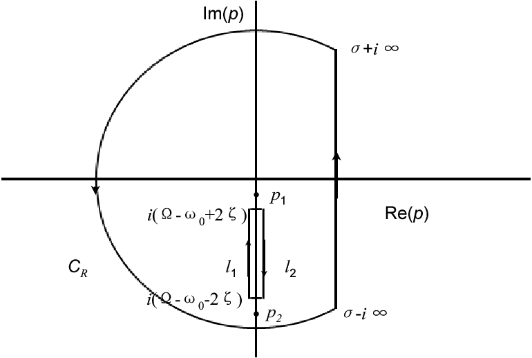
In the following, we will calculate $\alpha(t)$ by making use of the inverse Laplace transform,

\alpha(t)=\frac{1}{2\pi i}\int\limits_{\sigma-i\infty}^{\sigma+i\infty}dp\tilde{\alpha}(p)e^{pt}.

(85)

As shown in Fig. 8, the contour integration is divided into four parts as follows

\int\limits_{\sigma-i\infty}^{\sigma+i\infty}+\int\limits_{C_{R}}+\int\limits_{l_{1}}+\int\limits_{l_{2}}=\oint=\sum_{j}\mathrm{res}[\tilde{\alpha}(p_{j})e^{p_{j}t}]\text{,}

(86)

where $\mathrm{res}[F(p)]$ denotes the residue of function $F(p)$ at $p$ . Thus, we have

$\displaystyle\alpha(t)$	$\displaystyle=$	$\displaystyle\frac{1}{2\pi i}\int\limits_{\sigma-i\infty}^{\sigma+i\infty}dp\tilde{\alpha}(p)e^{pt}$	(87)
	$\displaystyle=$	$\displaystyle\sum_{j}\mathrm{res}[\tilde{\alpha}(p_{j})e^{p_{j}t}]-\int\limits_{C_{R}}-\int\limits_{l_{1}}-\int\limits_{l_{2}}$
	$\displaystyle=$	$\displaystyle\sum_{j}\mathrm{res}[\tilde{\alpha}(p_{j})e^{p_{j}t}]-\int\limits_{l_{1}}-\int\limits_{l_{2}}\text{,}$

where we have used the generalized Jordan Lemma [31]

\int\limits_{C_{R}}=0.

(88)

For the pole given by Eqs. (74) and (78), the residue is given as

\mathrm{res}[\tilde{\alpha}(p_{1})e^{p_{1}t}]=\frac{e^{p_{1}t}}{\frac{df_{1}(p)}{dp}|_{p=p_{1}}}=A_{1}e^{p_{1}t}\text{,}

(89)

where

A_{1}=\frac{[(ip_{1}+\frac{\Omega}{2}-\omega_{0})^{2}-4\zeta^{2}]}{[(ip_{1}+\frac{\Omega}{2}-\omega_{0})^{2}-4\zeta^{2}]+(ip_{1}-\frac{\Omega}{2})(ip_{1}+\frac{\Omega}{2}-\omega_{0})}\text{.}

(90)

For the singular point given by Eq. (84) and Eq. (80), the residue is given as

\mathrm{res}[\alpha(p_{2})e^{p_{2}t}]=\frac{e^{p_{2}t}}{\frac{df_{2}(p)}{dp}|_{p=p_{2}}}=A_{2}e^{p_{2}t}\text{,}

(91)

where

A_{2}=\frac{[(ip_{2}+\frac{\Omega}{2}-\omega_{0})^{2}-4\zeta^{2}]}{[(ip_{2}+\frac{\Omega}{2}-\omega_{0})^{2}-4\zeta^{2}]+(ip_{2}-\frac{\Omega}{2})(ip_{2}+\frac{\Omega}{2}-\omega_{0})}.

(92)

In the following we will calculate the contribution from the branch cut as

$\displaystyle-\int\limits_{l_{1}}-\int\limits_{l_{2}}$	$\displaystyle=$	$\displaystyle-\frac{1}{2\pi i}[\int\limits_{ip_{\min}}^{ip_{\max}}\frac{e^{pt}dp}{(p+i\frac{\Omega}{2})+\sum\limits_{k}\frac{g_{k}^{2}}{p\newline +i(\omega_{k}-\frac{\Omega}{2})-0^{+}}}$	(93)
		$\displaystyle+\int\limits_{ip_{\max}}^{ip_{\min}}\frac{e^{pt}dp}{(p+i\frac{\Omega}{2})+\sum\limits_{k}\frac{g_{k}^{2}}{p-i(\frac{\Omega}{2}-\omega_{k})+0^{+}}}]$
	$\displaystyle=$	$\displaystyle-\frac{1}{2\pi i}[\int\limits_{p_{\min}}^{p_{\max}}\frac{e^{ipt}dp}{(p+\frac{\Omega}{2})-\sum\limits_{k}\frac{g_{k}^{2}}{p-(\frac{\Omega}{2}-\omega_{k})+i0^{+}}}$
		$\displaystyle+\int\limits_{p_{\max}}^{p_{\min}}\frac{e^{ipt}dp}{(p+\frac{\Omega}{2})-\sum\limits_{k}\frac{g_{k}^{2}}{p-(\frac{\Omega}{2}-\omega_{k})-i0^{+}}}]\text{,}$

where the limits for the integral are

	$\displaystyle p_{\min}$	$\displaystyle=$	$\displaystyle\frac{\Omega}{2}-\omega_{0}-2\zeta\text{,}$		(94)
	$\displaystyle p_{\max}$	$\displaystyle=$	$\displaystyle\frac{\Omega}{2}-\omega_{0}+2\zeta\text{.}$		(95)

In the denominator of Eq. (93),

			$\displaystyle\sum\limits_{k}\frac{g_{k}^{2}}{p-(\frac{\Omega}{2}-\omega_{k})\pm i0^{+}}$
		$\displaystyle=$	$\displaystyle\frac{N}{2\pi}\int\limits_{-\pi}^{\pi}\frac{g_{k}^{2}dk}{p-(\frac{\Omega}{2}-\omega_{k})\pm i0^{+}}$
		$\displaystyle=$	$\displaystyle\frac{g^{2}}{2\pi}\int\limits_{-\pi}^{\pi}dk[\mathcal{P}\frac{1}{p-(\frac{\Omega}{2}-\omega_{k})}\mp i\pi\delta(p-\frac{\Omega}{2}+\omega_{k})]$
		$\displaystyle=$	$\displaystyle\frac{g^{2}}{2\pi}[\int\limits_{-\pi}^{\pi}dk\mathcal{P}\frac{1}{p-(\frac{\Omega}{2}-\omega_{k})}$
			$\displaystyle\mp i2\pi\int\limits_{\omega_{0}-2\zeta}^{\omega_{0}+2\zeta}\left\|\frac{dk}{d\omega_{k}}\right\|d\omega_{k}\delta(p-\frac{\Omega}{2}+\omega_{k})]$
		$\displaystyle=$	$\displaystyle\frac{g^{2}}{2\pi}[\int\limits_{-\pi}^{\pi}dk\mathcal{P}\frac{1}{p-(\frac{\Omega}{2}-\omega_{k})}$
			$\displaystyle\mp\int\limits_{\omega_{0}-2\zeta}^{\omega_{0}+2\zeta}\frac{i2\pi}{2\zeta\left\|\sin k\right\|}d\omega_{k}\delta(p-\frac{\Omega}{2}+\omega_{k})]$
		$\displaystyle=$	$\displaystyle\frac{g^{2}}{2\pi}[\int\limits_{-\pi}^{\pi}dk\mathcal{P}\frac{1}{p-(\frac{\Omega}{2}-\omega_{k})}$
			$\displaystyle\mp\int\limits_{\omega_{0}-2\zeta}^{\omega_{0}+2\zeta}\frac{i2\pi\delta(p-\frac{\Omega}{2}+\omega_{k})}{\sqrt{(2\zeta)^{2}-(\omega_{0}-\omega_{k})^{2}}}d\omega_{k}]$
		$\displaystyle=$	$\displaystyle\frac{g^{2}}{2\pi}[\int\limits_{-\pi}^{\pi}dk\mathcal{P}\frac{1}{p-(\frac{\Omega}{2}-\omega_{k})}\mp\frac{i2\pi}{\sqrt{(2\zeta)^{2}-(\omega_{0}+p-\frac{\Omega}{2})^{2}}}]\text{,}$

where the principal value function

\mathcal{P}\frac{1}{p-(\frac{\Omega}{2}-\omega_{k})}=\left\{\begin{array}[]{c}0\\ \frac{1}{p-(\frac{\Omega}{2}-\omega_{k})}\end{array}\right.\begin{array}[]{c}\text{if }p-(\frac{\Omega}{2}-\omega_{k})=0\\ \text{if }p-(\frac{\Omega}{2}-\omega_{k})\neq 0\end{array}\text{,}

(97)

and the additional factor $2$ in the fourth line is due to the same contribution from $\pm k$ .

And the first term on the right hand side of Eq. ()

$\displaystyle\int\limits_{-\pi}^{\pi}dk\mathcal{P}\frac{1}{p-(\frac{\Omega}{2}-\omega_{k})}$	$\displaystyle=$	$\displaystyle\int\limits_{-\pi}^{\pi}dk\mathcal{P}\frac{1}{p-\frac{\Omega}{2}+\omega_{0}-2\zeta\cos k}$
	$\displaystyle=$	$\displaystyle\oint\limits_{\left\|z\right\|=1}\frac{dz}{iz}\mathcal{P}\frac{1}{(p-\frac{\Omega}{2}+\omega_{0})-\zeta(z+\frac{1}{z})}$
	$\displaystyle=$	$\displaystyle\oint\limits_{\left\|z\right\|=1}\frac{dz}{-i\zeta}\mathcal{P}\frac{1}{z^{2}-\frac{p-\frac{\Omega}{2}+\omega_{0}}{\zeta}z+1}$
	$\displaystyle=$	$\displaystyle\frac{2\pi i}{-i\zeta}\sum\mathrm{res[}\frac{1}{z^{2}-\frac{p-\frac{\Omega}{2}+\omega_{0}}{\zeta}z+1}]\text{,}$

where the summation is over the residue within the loop enclosed by $\left|z\right|=1$ . Apparently, there are two solutions to the equation

z^{2}-\frac{p-\frac{\Omega}{2}+\omega_{0}}{\zeta}z+1=0\text{,}

(99)

i.e.,

z_{\pm}=\frac{M_{1}\pm i\sqrt{4-M_{1}^{2}}}{2}

(100)

with

M_{1}=\frac{p-\frac{\Omega}{2}+\omega_{0}}{\zeta}\text{.}

(101)

For the branch cut

p\in\left[\Omega/2-\omega_{0}-2\zeta,\Omega/2-\omega_{0}+2\zeta\right]\text{,}

(102)

we have

	$\displaystyle M_{1}$	$\displaystyle\in$	$\displaystyle[-2,2]\text{,}$		(103)
	$\displaystyle\left\|z_{\pm}\right\|$	$\displaystyle=$	$\displaystyle 1\text{.}$		(104)

Furthermore, due to the principal value function $\mathcal{P}$ , the above two singular points are removed from the integral path. As a result,

\int\limits_{-\pi}^{\pi}dk\mathcal{P}\frac{1}{p-(\frac{\Omega}{2}-\omega_{k})}=0\text{.}

(105)

Then, by substituting the above equation into Eq. (), we have

\sum\limits_{k}\frac{g_{k}^{2}}{p-(\frac{\Omega}{2}-\omega_{k})\pm i0^{+}}=\mp\frac{ig^{2}}{\sqrt{(2\zeta)^{2}-(\omega_{0}+p-\frac{\Omega}{2})^{2}}}\text{.}

(106)

Therefore, the contribution from the branch cut can be further simplified as

-\int\limits_{l_{1}}-\int\limits_{l_{2}}=\int\limits_{-2\zeta}^{2\zeta}C(x)e^{i(\frac{\Omega}{2}-\omega_{0}+x)t}dx

(107)

with

C(x)=\frac{1}{\pi}\frac{g^{2}\sqrt{4\zeta^{2}-x^{2}}}{(4\zeta^{2}-x^{2})(\Omega-\omega_{0}+x)^{2}+g^{4}}\text{.}

(108)

In conclusion, the final solution is written as

	$\displaystyle\alpha(t)$	$\displaystyle=$	$\displaystyle\sum_{j}\mathrm{res}[\alpha(p_{j})e^{p_{j}t}]-\int\limits_{l_{1}}-\int\limits_{l_{2}}$
		$\displaystyle=$	$\displaystyle A_{1}e^{p_{1}t}+A_{2}e^{p_{2}t}+\int\limits_{-2\zeta}^{2\zeta}C(x)e^{i(\frac{\Omega}{2}-\omega_{0}+x)t}dx\text{,}$

where the coefficients $A_{1}$ , $A_{2}$ , and $C(x)$ are real as given in Eqs. (90), (92), and (108) respectively. Here, two pure image numbers $p_{j}$ are the solutions to

\left(ip-\frac{\Omega}{2}\right)^{2}\left[\left(ip+\frac{\Omega}{2}-\omega_{0}\right)^{2}-4\zeta^{2}\right]+g^{4}=0

(110)

with

ip_{1}+\frac{\Omega}{2}-\omega_{0}>2\zeta,

(111)

and

ip_{2}+\frac{\Omega}{2}-\omega_{0}<-2\zeta.

(112)

The decay rate without measurement is defined as

R(t)=-\frac{d\left|\alpha(t)\right|^{2}}{dt}/\left|\alpha(t)\right|^{2}\text{,}

(113)

where the survival probability for the initial state is

\left|\alpha(t)\right|^{2}=\left|A_{1}e^{p_{1}t}+A_{2}e^{p_{2}t}+\int\limits_{-2\zeta}^{2\zeta}C(x)e^{i(\frac{\Omega}{2}-\omega_{0}+x)t}dx\right|^{2}

(114)

and its rate of change is

$\displaystyle\frac{d\left\|\alpha(t)\right\|^{2}}{dt}$	$\displaystyle=$	$\displaystyle 2\Re(I_{1}\times I_{2}^{\ast})$	(115)
		$\displaystyle-2A_{1}A_{2}(ip_{1}-ip_{2})\sin(ip_{1}-ip_{2})t$
		$\displaystyle+2\Re[(A_{1}p_{1}e^{p_{1}t}+A_{2}p_{2}e^{p_{2}t})I_{1}^{\ast}]$
		$\displaystyle+2\Re[(A_{1}e^{p_{1}t}+A_{2}e^{p_{2}t})I_{2}^{\ast}],$

where the integrals are defined as

	$\displaystyle I_{1}$	$\displaystyle=$	$\displaystyle\int\limits_{-2\zeta}^{2\zeta}C(x)e^{i(\frac{\Omega}{2}-\omega_{0}+x)t}dx,$		(116)
	$\displaystyle I_{2}$	$\displaystyle=$	$\displaystyle\int\limits_{-2\zeta}^{2\zeta}C(x)e^{i(\frac{\Omega}{2}-\omega_{0}+x)t}i(\frac{\Omega}{2}-\omega_{0}+x)dx,$		(117)

and $\Re(x)$ is the real part of $x$ .

References

[1] H. P. Breuer, F. Petruccione, The Theory of Open Quantum Systems (Oxford University Press, Oxford, New York, 2002).
[2] L. H. Yu, and C. P. Sun, Phys. Rev. A 49, 592 (1994).
[3] C. P. Sun, and L. H. Yu, Phys. Rev. A 51, 1845 (1995).
[4] L. S. Khalhin, JETP Lett. 8, 65 (1968).
[5] B. Misra and E. C. G. Sudarshan, J. Math. Phys. (N.Y.) 18, 756 (1977).
[6] K. Koshinoa and A. Shimizuc, Phys. Rep. 412, 191 (2005).
[7] A. G. Kofman and G. Kurizki, Nature (London) 405, 546 (2000).
[8] M. C. Fischer, B. Gutiérrez-Medina, and M. G. Raizen, Phys. Rev. Lett. 87, 040402 (2001).
[9] N. Bar-Gill, E. E. Rowen, G. Kurizki, and N. Davidson, Phys. Rev. Lett. 102, 110401 (2009).
[10] L. Zhou, Z. R. Gong, Yu-xi Liu, C. P. Sun, and F. Nori, Phys. Rev. Lett. 101, 100501 (2008).
[11] L. Zhou, S. Yang, Yu-xi Liu, C. P. Sun, and F. Nori, Phys. Rev. A 80, 062109 (2009).
[12] H. Zheng, S. Y. Zhu, and M. S. Zubairy, Phys. Rev. Lett. 101, 200404 (2008).
[13] Q. Ai, Y. Li, and C. P. Sun, arXiv:1003.1899 (2010).
[14] M. O. Scully and M. S. Zubairy, Quantum Optics (Cambridge University Press, Cambridge, England, 1997).
[15] H. B. Zhu and C. P. Sun, Science in China (A) 30 , 928 (2000); Progeresses in Natural Sciences 10, 698, (2000).
[16] H. Fröhlich, Phys. Rev. 79, 845 (1950); Proc. Roy. Soc. A 215, 291 (1952); Adv. Phys. 3, 325 (1954).
[17] S. Nakajima, Adv. Phys. 4, 363 (1953).
[18] C. P. Sun, Y. D. Wang, Y. Li, and P. Zhang, in Recent Progress in Quantum Mechanics Vol. III, edited by J. Y. Zeng, G. L. Long, and S. Y. Pei (Tsinghua University Press, Beijing, 2003), p. 139.
[19] R. Loudon and S. M. Barnett, J. Phys. B: At. Mol. Opt. Phys. 39, S555 (2006).
[20] L. V. Hove, Phys. Rev. 89, 1189 (1953).
[21] A. Blais, R. S. Huang, A. Wallraff, S. M. Girvin, and R. J. Schoelkopf, Phys. Rev. A 69, 062320 (2004).
[22] J. Q. Liao, J. F. Huang, Y. X. Liu, L. M. Kuang, and C. P. Sun, Phys. Rev. A 80, 014301 (2009); J. Q. Liao, Z. R. Gong, L. Zhou, Y. X. Liu, C. P. Sun, and F, Nori, Phys. Rev. A, in press (2010).
[23] A. Wallraff, D. I. Schuster, A. Blais, L. Frunzio, R. -S. Huang, J. Majer, S. Kumar, S. M. Girvin and R. J. Schoelkopf, Nature 431, 162 (2004).
[24] Y. Akahane, T. Asano, B.-S. Song, and S. Noda, Nature 425, 944 (2003).
[25] T. Yoshie, A. Scherer, J. Hendrickson, G. Khitrova, H. M. Gibbs, G. Rupper, C. Ell, O. B. Shchekin, and D. G. Deppe, Nature 432, 200 (2004).
[26] D. Englund, A. Majumdar, A. F. M. Toishi, N. Stoltz, P. Petroff, and J. Vuc̆ković, Phys. Rev. Lett. 104, 073904 (2010).
[27] X. D. Yang, M. B Yu, D.-L. Kwong, and C. W. Wong, Phys. Rev. Lett. 102, 173902 (2009).
[28] D. Z. Xu, H. Ian, T. Shi, H. Dong, and C. P. Sun, arXiv:0812.0429 (2008).
[29] I. Lizuain, J. Casabiva, J. J. Carcía-Ripoll, J. G. Muga, and E. Solano, arXiv:0912.3485 (2009).
[30] W. M. Itano, D. J. Heinzen, J. J. Bollinger, and D. J. Wineland, Phys. Rev. A 41, 2295 (1990).
[31] K. M. Liang, Method of Mathematical Physics (Higher Education Press, Beijing, China, 1998).