Granular Brownian motion
Abstract
We study the stochastic motion of an intruder in a dilute driven granular gas. All particles are coupled to a thermostat, representing the external energy source, which is the sum of random forces and a viscous drag. The dynamics of the intruder, in the large mass limit, is well described by a linear Langevin equation, combining the effects of the external bath and of the “granular bath”. The drag and diffusion coefficients are calculated under few assumptions, whose validity is well verified in numerical simulations. We also discuss the non-equilibrium properties of the intruder dynamics, as well as the corrections due to finite packing fraction or finite intruder mass.
1 Introduction
Granular materials in the fluidized state [1, 2] have represented, during the last 10-15 years, an excellent benchmark for new and old theories in non-equilibrium statistical mechanics: the presence of non-conservative forces make unavailable the standard tools used at equilibrium, such as Gibbs measure, equipartition, thermodynamic limit, Einstein relation and more [3, 4, 5, 6]. It is therefore necessary to resort to more fundamental theories, from the Boltzmann equation up to stochastic processes and modern generalizations of statistical mechanics to non-equilibrium states [7, 8].
In order to achieve a stationary state, the fundamental ingredient is an external source of energy, required to compensate the energy lost in inelastic collisions. The role of energy source is played by some injection mechanisms, depending upon the experimental setup, e.g.: a box with a vibrating wall, a layer (or more than one) placed over a vibrating plate, a gas flux going through orifices in the box walls, etc. The different mechanisms may produce quite different states with different symmetries: for instance a layer over a vibrating plate is homogeneous on average, while a boundary driving (e.g. a shaken box wall) leads to spatial gradients and currents [9, 10, 11].
From the point of view of a tracer particle, however, the dynamics is always of a similar kind: the tracer interacts, in a random sequence, with the surrounding particles and with the energy source. The ratio between frequencies of interaction dictates the relevance of tracer-particle collisions with respect to exchanges between the tracer and the source. Of course, in a boundary-driven setup, the statistics of collisions suffered by the tracer depends upon the distance from the energy source. Anyway, the random motion performed by the granular tracer should always take into account the two contributions: collisions with other granular particles and interaction with the energy source. In more idealized setups, the so-called Homogeneous or non-Homogeneous Cooling States, no energy injection is involved: in this regimes, anyway, a collisional stationary state cannot be achieved and experimental verification is very difficult to be achieved.
Here we consider a model commonly used in the theoretical literature on granular fluids: all grains are coupled to a thermostat-like energy source, with a typical interaction time which is usually taken larger than the inter-particles collision time [12, 13]. The stationary granular gas obtained in this way, is then used as a “granular bath” where a massive intruder performs a non-equilibrium Brownian motion, still being coupled to external energy source. The result is a double bath whose properties are analyzed starting from a linear Boltzmann-Lorentz-Fokker-Planck equation, which is treated in the diffusional approximation (large mass) to be cast into a Langevin equation.
Self-diffusion of an intruder [14, 15] or a tracer [16, 17] has been previously studied in the Homogeneous Cooling State. The same calculations have been performed for models with an impact velocity dependent restitution coefficient [18] and a good review of main results can be found in the textbook [8]. Diffusion in a stationary granular fluid obtained by imposing shear boundary conditions has also been considered [19].
Up to our knowledge this is the first time that self-diffusion of a large mass intruder is studied for a model with homogeneous energy injection, considering explicitly the effect of a “double bath”, i.e. of both sources of noise, granular and external respectively. A Langevin equation (31) with expressions for the tracer temperature, Eq. (34), mobility, Eq. (32), and diffusion coefficients, Eq. (35), all involve the interplay of both energy sources. The large mass limit, together with the Molecular Chaos assumption (due to diluteness) guarantees that a granular Fluctuation-Dissipation theorem holds, where the ratio between diffusion and mobility is simply given by the intruder granular temperature [20, 21].
In Section 2 we introduce the model (granular gas, thermostat and intruder); in Section 3 the Kramers-Moyal expansion and the large mass limit are discussed, leading to the Langevin formulation in Section 3.2. Numerical experiments (Molecular Dynamics and Direct Simulation Monte Carlo) are performed to study the limits of the used assumptions in Section 4 and finally conclusions and perspectives are drawn in Section 5.
2 The model
We consider a gas of granular spheres in dimensions, each sphere has index , with , and mass . Particle (referred to as “the intruder”) has mass and radius , while all other particles (usually denoted as “the gas”) have mass and radius . The parameter will be used for large mass expansion. The system is contained in a box of volume , much greater than the volume occupied by the particles, so that the hypothesis of molecular chaos applies. We denote by the density of the gas and by the occupied volume fraction (in it is, for instance, ).
The intruder and the gas particles undergo binary instantaneous inelastic collisions when coming at contact, with the following rule
| (1) | |||||
| (2) |
where () and () are the post and pre-collisional velocities of particle (particle ), respectively; is the restitution coefficient 11 1 for simplicity we consider the restitution coefficient to be equal for all particles., and is the unit vector joining the centers of the colliding particles. The mean free path of the intruder is . Two kinetic temperatures can be introduced for the two species: the gas granular temperature () and the intruder granular temperature .
In order to maintain a fluidized granular gas, an external energy source is coupled to every particle in the form of a thermal bath. The motion of a particle with velocity is then described by the following stochastic equation
| (3) |
Here is the force taking into account the collisions with other particles, and is a white noise, with and , where Latin indices refer to particle labels while Greek indices denote Cartesian coordinates 22 2 We use a constant , but in principle this coefficient may depend on the mass and on the radius of the particle, since it is only a model description of a more complicate interaction with plates, walls or fluids going through the granular medium..
The effect of the external energy source balances the energy lost in the collisions and a stationary state is attained. Several temporal scales are important in this system:
- •
, the mean free time between collisions of a gas particle;
- •
, the mean free time between collisions of the intruder;
- •
the typical interaction time of the bath with gas particles;
- •
the typical interaction time of the bath with the intruder.
When is small enough to have the mean free times and smaller than the interaction times and , inelasticity is sufficient to put the gas out of equilibrium: this is reflected, among other things, in the failure of equipartition and . It is also known that [22, 23].
The main goal of this note is to show that, in the limit of large mass , the force acting on the intruder can be expressed by means of a Langevin-like formula , providing explicit expressions for and .
In order to do that, let us start by writing the coupled Boltzmann equations for the probability distributions and , denoting (for simplicity) with and the intruder velocity and the gas velocity, respectively
| (4) | |||||
where and are two operators taking into account the interactions with the thermal bath. In these equations the effects of the collisions for the tracer and the gas particles are described by, respectively,
| (5) | |||||
and
| (6) | |||||
where is the Heaviside step function, is the Dirac delta function in dimensions, and , being the pair correlation function for a gas particle and an intruder at contact; in the expressions (5) and (6) we have assumed that the probability that a collision between the intruder and a gas particle occurs, when they have velocities and and positions and respectively, is given by the Enskog approximation [8]
| (7) |
which is a small correction to Molecular Chaos, taking into account density correlations near the intruder; the terms describing the action of the thermal bath read
| (8) | |||
| (9) |
where is the Laplacian operator with respect to the velocity; finally, the Boltzmann collision operator for the particle-particle interactions , can be found in many papers, see for instance [24]. In view of the fact that it is not relevant for the rest of the paper, we omit its explicit expression.
2.1 Decoupling the gas from the tracer
The two Boltzmann equations appearing in the system (4) are coupled through the terms involving and . Nevertheless, if the number of granular particles is large enough, the term can be neglected because of the factor in Eq. (6). Hence, the surrounding gas is weakly perturbed by the tracer and fast and homogeneous relaxation is expected. One assumes that the probability distribution function is stationary and, following numerical evidence (verified below) it is approximated with a Gaussian function with variance :
| (10) |
Substituting Eq. (10) into Eq. (5), and projecting the velocities along the collision direction and the orthogonal one, the integral can be solved [25], yielding
where (note that is parallel to ) and . From now on we specialize to the two dimensional case, where the above equation simplifies to
| (12) | |||||
As discussed in details below, once the gas is decoupled from the intruder, the dynamics of the tracer alone is Markovian, and it is known that such transition rates satisfy detailed balance with respect to a Gaussian invariant probability [25] (the temperature of the tracer, in that case, where , is given by [26]).
2.2 Granular temperature of the gas
The granular temperature can be obtained from the Langevin equation (3). Indeed, multiplying by and averaging, one gets
| (13) |
At stationarity, the l.h.s. of the above equation vanishes and . The term represents the average power dissipated by collisions, which we assume to be dominated (this is true for large enough) by gas-gas collisions:
| (14) |
where is the energy dissipated per particle and the collision average is defined by
where and is the mean free path for gas-gas collisions and is the pair correlation function for two gas particles at contact. The integral in Eq. (14) can be computed by standard methods [8], and, in two dimensions, yields
| (15) |
Substituting this result into Eq. (13) and recalling that , one finally obtains the implicit equation
| (16) |
which can be solved to obtain .
3 Kramers-Moyal expansion for the tracer-gas collision operator
With the assumption discussed above, the system of equations (4) is decoupled. That allows us to write the following linear Master Equation for the tracer
| (17) |
where is a linear operator which can be expressed by means of the Kramers-Moyal expansion [27]
| (18) |
(the sum over repeated indices is meant) with
| (19) |
and is given by relation (12). The second term in the Master Equation represents the interaction with thermal bath:
| (20) |
In the limit of large mass , i.e. small , we expect that the interaction between the granular gas and the tracer can be described by means of an effective Langevin equation. In this case, we keep only the first two terms of the expansion [27]
| (21) |
A justification of this truncation, in the limit of small , comes from observing that terms are of order : this can be obtained by plugging Eqs. (1) (for the case of the tracer, i.e. ) into (19).
It is useful at this point to introduce the velocity-dependent collision rate and the total collision frequency
| (22) | |||||
| (23) |
The former quantity can be exactly calculated, giving
| (24) | |||||
where the rescaled variable is introduced in Appendix through Eqs. (54) and are the modified Bessel functions. To have an approximation of , on the other side, one has to make a position about . Let us take it to be a Gaussian with variance . The consistency of this choice will be verified in the following section. With this assumption, the collision rate turns out to be
| (25) |
where and .
3.1 Large mass limit
We are then able to compute the terms and appearing in . The result and the details of the computation of these coefficients as functions of are given in Appendix. Here, in order to be consistent with the approximation in (21), from Eqs. (55) we report only terms up to
| (26) | |||||
| (27) | |||||
| (28) | |||||
| (29) |
The linear dependence of upon (for each component ), allows a granular viscosity
| (30) |
In the elastic limit , one retrieves the classical results: and . In this limit the Fluctuation-Dissipation relation of the second kind is satisfied [28, 29], i.e. the ratio between the noise amplitude and , associated to the same source (collision with gas particles), is exactly . When the collisions are inelastic, , one sees two main effects: 1) the time scale associated to the drag is modified by a factor , i.e. it is weakly influenced by inelasticity; 2) the Fluctuation-Dissipation relation of the second kind is violated by the same factor . This is only a partial conclusion, which has to be re-considered in the context of the full dynamics, including the external bath: this is discussed in the next section.
3.2 Langevin equation for the tracer
Putting together the results in Eqs. (26-29) with Eqs. (17-21), we are finally able to write the Langevin equation for the tracer
| (31) |
where and , with
| (32) | |||||
| (33) |
concluding that the stationary velocity distribution of the intruder is Gaussian with temperature
| (34) |
Equation (31) is consistent with the Gaussian ansatz used in computing . Note that the above expression for is consistent with the large mass expansion obtained in Eqs. (29) only if it is dominated by , for instance when (see discussion at the end of A). In the opposite limit, the tracer dynamics is dominated by the coupling with the external bath and the typical velocity of the tracer cannot be taken sufficiently small with respect to the typical velocity of gas particles, making the expansion unreliable. In this case, however, if the diameter of the intruder is similar to that of the gas particles, it is reasonable to expect similar collision frequencies: the gas particles will therefore be dominated by the external bath and the whole system will be very near to equilibrium [30, 12].
For the self-diffusion coefficient it is immediately obtained
| (35) |
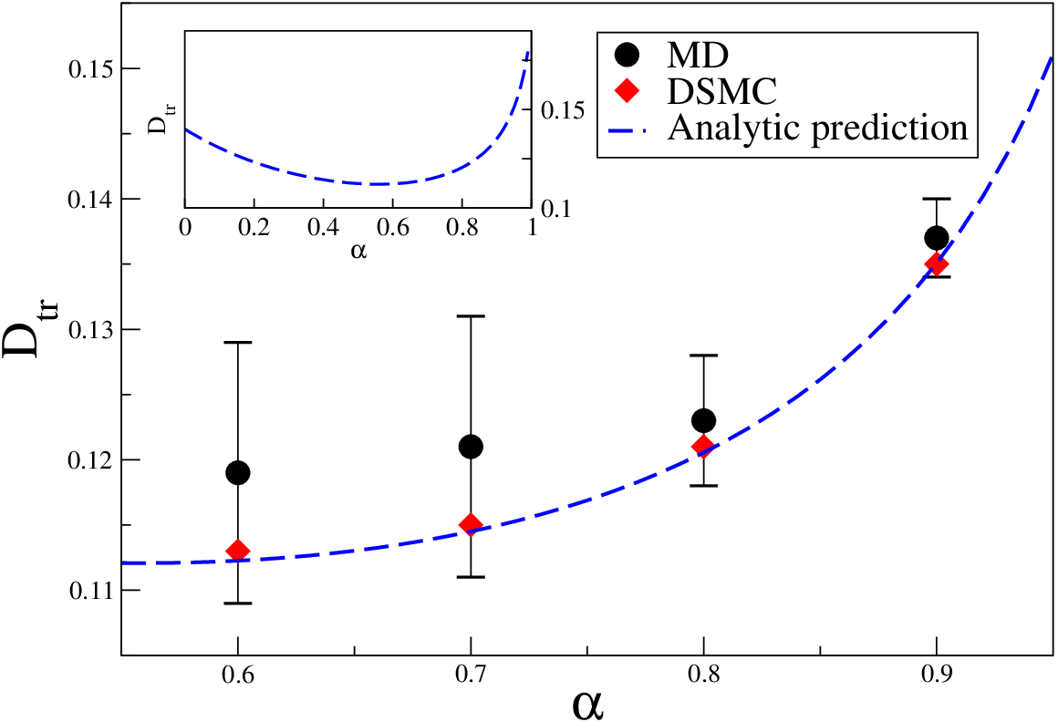
Solving numerically the equation (16) and substituting the result into the above equation, one can study as a function of the restitution coefficient (this is done numerically in the next section). When all other parameters are kept constant and is reduced from , the behavior of is non-monotonic, it decreases, has a minimum and then increases for lower values of . Anyway, this minimum is expected for quite low values of or high values of the packing fraction , where the approximations involved in this theory are not good. For this reason, at the values of parameters chosen to have a good comparison with simulations, this non-monotonic behavior is not observed.
It should be also noticed that, in the Homogeneous Cooling State, the self-diffusion coefficient at a given granular temperature increases as is reduced from , i.e. it has an opposite behavior with respect to the present case [14, 15]. Other studies on different models of driven granular gases have found expressions very close to Eq. (32), which is not surprising considering the universality of the main ingredient for this quantity, i.e. the collision integral [5, 31].
3.3 Energy fluxes and detailed balance
A few comments are in order, at this point, concerning the non-equilibrium properties of this system. The first question comes about the term which multiplies in Eq. (34). It is easily explained with the following argument [25]: we have assumed that the tracer feels no memory of past collisions, which means that any post-collisional correlation with recoiling gas particles is lost. With these assumption, the fate of recoiling particles can be ignored and the dynamics concerns only the intruder:
| (36) |
where is the pre-collisional velocity of the colliding gas particle (randomly extracted from the given distribution ). Then, one simply observes that for any value of , and , such rule can be rewritten as an elastic collision rule with an effective mass for large intruder mass. This is equivalent to say that the tracer has elastic interactions with the gas particles, with an effective mass , and therefore feels an effective temperature of the gas . Note that this argument, for , gives the formula , which has been derived for the first time in [26].
The energy injection rates of the two thermostats [32] are
| (37) | |||||
| (38) |
It is easy to see that the balance of fluxes is equivalent to formula (34) for . This balance implies that, if , then . When , the two fluxes are different from zero, i.e. energy is flowing from the external driving, through the tracer, into the granular bath.
Apparently, this contradicts the “equilibrium” nature of the Langevin equation (31): the tracer dynamics is Markovian and stationary, and the equation satisfies detailed balance with respect to the Gaussian invariant distribution. As already discussed in [25], this is not a paradox but only a consequence of Molecular Chaos and the decoupling assumption which allows us to write Equation (17): here we have employed the Enskog approximation, which is a weak modification of Molecular Chaos, still preserving Markovianity, i.e. no memory terms appear in Eq. (4). The absence of memory implies that both and are white noises and makes them indistinguishable: an observer which can only measure cannot obtain separate measures of and , but only a measure of the total energy flow which hides out the presence of energy currents. A more detailed analysis, e.g. by relaxing the Enskog approximation, should put in evidence the different time-correlations of the two baths: eventually, the observer, by means of some “filter”, should be able to sort out their different contributions and . This is an interesting example where memory plays a crucial role in the non-equilibrium characterization of a system [33].
We expect that time reversibility (detailed balance) is a symmetry, for the intruder, which is broken in the following cases: 1) at small values of (this is different from the case discussed in [25], where the intruder was not in contact with the external bath); 2) when the non-Gaussian behavior of the gas velocities is taken into account; 3) when the tracer has asymmetric properties with respect to some spatial axis [34]; 4) when Molecular Chaos (or its weak Enskog correction) is violated [5].
4 Numerical simulations
In this Section we report the results of Molecular Dynamics (MD) simulations of the model, together with Direct Simulation Monte Carlo (DSMC) simulations [35] incorporating the Enskog correction, and compare them with our theoretical predictions. In all simulations we have kept constant the dimension , the mass of gas particles and the radii , as well as the properties of the bath and ; instead we have varied , , and (values of and can be obtained from the knowledge of and ). We have used the Carnahan-Starling expression for at contact [36]: . For the chosen values of , it is always . In all simulations we have also checked that the Gaussian approximations for the velocity distributions of gas particles and for the intruder are satisfied, observing very small values for the second Sonine coefficient [8].
In Fig. 1 we show the velocity-velocity autocorrelation function of the tracer for different values of its mass in a dilute and moderately inelastic case: , and (and for MD). We can clearly observe that in the case of large mass the Langevin equation (31) describes very well the dynamics of the tracer. Indeed, in that case, the numerical results are consistent with the theoretical prediction
| (39) |
As expected, for smaller values of , the numerical results move away from the analytical ones and large corrections to the exponential decay do appear. The deviations are observed (and are quantitatively similar) for both MD and DSMC results, implying that they are due, as expected, to the breakdown of the large mass expansion, rather than that of Molecular Chaos. For MD results we have noticed that, going from to , the comparison with DSMC (and with theory at large ) is improved.


In order to check the validity of the hypothesis of molecular chaos, we report the results of MD and DSMC simulations for higher packing fractions in Fig. 2, keeping , (in MD) and : since the clean part of the decay of is always exponential, we focus only on the two parameters of interest, i.e. and . One clearly observes that, increasing the packing fraction, the discrepancy between the theoretical value and the values obtained from MD, increases. On the other side, DSMC always gives results very close to theory, as expected. The Enskog approximation (7), which does not take into account memory effects, is no longer valid in MD at high packing fraction, while always holds in DSMC. In order to enforce this statement, we computed the following correlation coefficient: , where we introduced the stochastic variable given by the averaged -component velocity of the particles lying, at time t, in a fixed area around the tracer. In particular, and measure the deviations of and from the average values, which tend to for a large number of measures. The coefficient defined above must be zero, if molecular chaos holds; on the contrary we observed that its value sensibly increases as the packing fraction gets higher. For example for , whereas, for , .

Finally let us compare the diffusion coefficient measured in MD and DSMC with the theoretical value obtained through Eqs. (16) and (35). In Fig. 3 we show our results at different values of , keeping fixed , and (in MD). Again there is a perfect match for DSMC, while MD simulations present a small discrepancy which becomes more evident at small values of . We have again verified that this discrepancy is a finite effect and is reduced as increases.
5 Conclusions
While many papers have been devoted to the large-mass diffusive properties of an intruder in a cooling granular gas, the driven case, somehow, has received less attention [19]: this is in contrast with the fact that, in real experiments, the most common situation is a driven granular gas. The problem, at the level of the basic assumptions treated here (Enskog approximation, negligible non-Gaussianity and large separation of timescales between collisions and driving), does not pose particular conceptual difficulties, nevertheless it reveals to be already quite rich. The external driving mechanism, characterized by a temperature and the “internal” granular bath at temperature , sum up together in giving a linear Langevin dynamics for the intruder, provided that the collision frequency between the intruder and the gas particles is larger than the frequency of interaction with the bath. Such Langevin equation predicts for the “intruder temperature” a weighted sum (with weights given by the drag coefficients of the two baths) of and , i.e. the intruder feels the surrounding gas to be at a different temperature , because of non-conservative interactions. The self-diffusion coefficient is even more interesting, showing a non-trivial non-monotonic behavior with a minimum at low values of the restitution coefficient. Our results lose validity when the mass of the intruder is reduced, when the packing fraction of the gas is increased, when the inelasticity is too low to disregard non-Gaussian corrections, and when the interaction times of the two baths become comparable.
It is interesting to discuss what is happening at moderately high packing fractions : we have seen that the Enskog approximation is not very good to predict the intruder dynamics, because it is missing memory effects mediated by the surrounding fluid. A scenario which can be conjectured is the following: the gas may display two typical relaxation times, a local one related to collisions and a global one , which is due to diffusion of slower modes (e.g. hydrodynamics). If , one has that the intruder feels a “locally equilibrated” surrounding granular gas. In this case it is reasonable to replace Eq. (10) with
| (40) |
where and are some local velocity and temperature fields which change on timescales larger than (and correspondingly large spatial scales). A partial verification of this scenario has been mentioned at the end of [5], but requires further investigation.
Appendix A Calculation of first two coefficients of the Kramers-Moyal expansion
For larger generality (whose motivation is discussed in the Conclusions), in this Appendix we discuss the case where the gas surrounding the intruder may have a non-zero average 33 3 note that in all the cases discussed in the main text, we have always taken .:
| (41) |
which is a simple task involving only the definition of new shifted variables
| (42) | |||||
| (43) |
We are interested in computing
| (44) | |||||

In order to perform the integral, we make the following change of variables (see Fig. 4 for an example)
| (45) |
which implies
| (46) |
where
| (47) |
is the Jacobian of the transformation. The collision rate is then
| (48) |
where are the modified Bessel functions. For we can write
| (49) | |||||
where we have enforced the constraint of the theta function, namely , with . Notice that the integral in is lower bounded by the condition which follows from the definition of . In order to compute the integral, we have to invert the transformation (45). That yields two determinations for the variables and (see Fig. 4)
Then the integral (49) can be written as
yielding
Analogously, for the coefficients one obtains
Then we introduce the rescaled variables
| (54) |
obtaining
| (55) | |||||
Up to this last results we have not introduced any small approximation. The next step consists in assuming that with respect to , which is equivalent to assume that : this assumption must be compared to its consequences, in particular to Eq. (34); the assumption is good for not too small values of and for , i.e. when . When this is the case, expanding in and using that and for small , one finds Eqs. (29).
References
References
- [1] H. M. Jaeger, S. R. Nagel, and R. P. Behringer. Granular solids, liquids, and gases. Reviews of Modern Physics, 68:1259, 1996.
- [2] T. Pöschel and S. Luding, editors. Granular Gases, Berlin, 2001. Springer. Lecture Notes in Physics 564.
- [3] I Goldhirsch. Scales and kinetics of granular flows. Chaos, 9:659, 1999.
- [4] L P Kadanoff. Built upon sand: Theoretical ideas inspired by granular flows. Rev. Mod. Phys., 71:435, 1999.
- [5] A Puglisi, A Baldassarri, and A Vulpiani. Violations of the Einstein relation in granular fluids: the role of correlations. J. Stat. Mech., page P08016, 2007.
- [6] J J Brey, M I G de Soria, and P Maynar. Breakdown of the fluctuation-dissipation relations in granular gases. Europhys. Lett., 84:24002, 2008.
- [7] T P C van Noije and M H Ernst. Velocity distributions in homogeneous granular fluids: the free and the heated case. Granular Matter, 1:57–64, 1998.
- [8] N K Brilliantov and T Poschel. Kinetic Theory of Granular Gases. Oxford University Press, 2004.
- [9] E. L. Grossman, T. Zhou, and E. Ben-Naim. Towards granular hydrodynamics in two-dimensions. Phys. Rev. E, 55:4200, 1997.
- [10] D R M Williams and F C MacKintosh. Driven granular media in one dimension: Correlations and equation of state. Phys. Rev. E, 54:R9, 1996.
- [11] A Puglisi, F Cecconi, and A Vulpiani. Models of fluidized granular materials: examples of non-equilibrium stationary states. J. Phys.: Condens. Matter, 17:2005, S2715.
- [12] A Puglisi, V Loreto, U M B Marconi, A Petri, and A Vulpiani. Clustering and non-gaussian behavior in granular matter. Phys. Rev. Lett., 81:3848, 1998.
- [13] F Cecconi, F Diotallevi, U Marini Bettolo Marconi, and A Puglisi. Fluid-like behavior of a one-dimensional granular gas. J. Chem. Phys., 120:35, 2004.
- [14] J J Brey, J W Dufty, and A Santos. Kinetic models for granular flow. J. Stat. Phys., 97:281, 1999.
- [15] J J Brey, M J Ruiz-Montero, R Garcia-Rojo, and J W Dufty. Brownian motion in a granular gas. Phys. Rev. E, 60:7174, 1999.
- [16] J J Brey, M J Ruiz-Montero, D Cubero, and R Garcia-Rojo. Self-diffusion in freely evolving granular gases. Phys. Fluids, 12:876, 2000.
- [17] V Garzó and J M Montanero. Diffusion of impurities in a granular gas. Physical Review E, 69:021301, 2004.
- [18] Nikolai V. Brilliantov and Thorsten Poschel. Self-diffusion in granular gases: Green–Kubo versus Chapman–Enskog. Chaos, 15:026108, 2005.
- [19] V Garzó. Tracer diffusion in granular shear flows. Phys. Rev. E, 66:021308, 2002.
- [20] A Puglisi, A Baldassarri, and V Loreto. Fluctuation-dissipation relations in driven granular gases. Physical Review E, 66:061305, 2002.
- [21] G. D’Anna, P. Mayor, G. Gremaud, A. Barrat, V. Loreto, and F. Nori. Observing brownian motion in vibration-fluidized granular matter. Nature, 424:909, 2003.
- [22] K Feitosa and N Menon. Breakdown of energy equipartition in a 2d binary vibrated granular gas. Phys. Rev. Lett., 88:198301, 2002.
- [23] R Pagnani, U Marini Bettolo Marconi, and A Puglisi. Driven low density granular mixtures. Phys. Rev. E, 66:051304, 2002.
- [24] V Garzó and José María Montanero. Transport coefficients of a heated granular gas. Physica A, 313:336, 2002.
- [25] A Puglisi, P Visco, E Trizac, and F van Wijland. Dynamics of a tracer granular particle as a nonequilibrium markov process. Phys. Rev. E, 73:021301, 2006.
- [26] P A Martin and J Piasecki. Thermalization of a particle by dissipative collisions. Europhys. Lett., 46:613, 1999.
- [27] H Risken. The Fokker-Planck equation: Methods of solution and applications. Springer- Verlag, Berlin, 1989.
- [28] R Kubo, M Toda, and N Hashitsume. Statistical physics II: Nonequilibrium stastical mechanics. Springer, 1991.
- [29] U Marini Bettolo Marconi, A Puglisi, L Rondoni, and A Vulpiani. Fluctuation-dissipation: Response theory in statistical physics. Phys. Rep., 461:111, 2008.
- [30] W Losert, D G W Cooper, J Delour, A Kudrolli, and J P Gollub. Velocity statistics in excited granular media. Chaos, 9:682, 1999.
- [31] G Bunin, Y Shokef, and D Levine. Frequency-dependent fluctuation-dissipation relations in granular gases. Phys. Rev. E, 77:051301, 2008.
- [32] P Visco. Work fluctations for a Brownian particle between two thermostats. J. Stat. Mech., page P06006, 2006.
- [33] A Puglisi and D Villamaina. Irreversible effects of memory. Europhys. Lett., 88:30004, 2009.
- [34] G Costantini, A Puglisi, and U Marini Bettolo Marconi. A granular brownian ratchet model. Phys. Rev. E, 75:061124, 2007.
- [35] G. A. Bird. Molecular Gas Dynamics and the Direct Simulation of Gas Flows. Clarendon, Oxford, 1994.
- [36] N F Carnahan and K E Starling. Equation of state for nonattracting rigid spheres. J. Chem. Phys., 51:635, 1969.