Exploring complex phenomena using ultracold atoms in bichromatic lattices
Abstract
With an underlying common theme of competing length scales, we study the many-body Schrödinger equation in a quasiperiodic potential and discuss its connection with the Kolmogorov-Arnold-Moser (KAM) problem of classical mechanics. We propose a possible visualization of such connection in experimentally accessible many-body observables. Those observables are useful probes for the three characteristic phases of the problem: the metallic, Anderson and band insulator phases. In addition, they exhibit fingerprints of non-linear phenomena such as Arnold tongues, bifurcations and devil’s staircases. Our numerical treatment is complemented with a perturbative analysis which provides insight on the underlying physics. The perturbation theory approach is particularly useful in illuminating the distinction between the Anderson insulator and the band insulator phases in terms of paired sets of dimerized states.
pacs
03.75.Ss, 05.45.-a, 37.10.JkI Introduction
Ultracold atoms are emerging as a versatile arena for the study of a variety of problems in physics. These clean and highly controllable systems can be viewed as simulators of complex quantum phenomena with applications in condensed matter, quantum optics, atomic and molecular physics and nonlinear dynamics, as well as in particle physics and cosmology [1, 2]. Some examples of this trend are the laboratory realization of the superfluid to Mott insulator transition with bosons [3], observation of the corresponding metal to Mott insulator transition with fermions [4, 5] and the creation of the Tonks-Girardeau gas in one dimensional systems [6, 7]. Ultracold atoms have also provided a laboratory realization of Wannier-Stark ladders [8] and the kicked-rotor model [9], a paradigm in the study of classical and quantum chaos [10]. Recent successful loading of atoms in a bichromatic optical lattice geometries [11], has opened new avenues for the study of phenomena where the competition between various length scales is at the heart of the problem.
Systems with competing lengths have fascinated physicists as well as mathematicians in view of their exotic fractal characteristics [12, 13]. Such systems with two competing periodicities, commonly known as almost-periodic or quasiperiodic, occur very commonly in nature. The most commonly studied example in quantum physics is the single particle Schrödinger equation in the presence of a quasiperiodic (QP) potential.
Motivated by experimental realization of two-color lattices, we revisit the problem of the Schrödinger equation in a quasiperiodic potential and its relationship with the Kolmogorov-Arnold-Moser (KAM) [14] problem of classical mechanics. Our particular focus is the treatment of many-body effects that are present in QP systems that have been extensively studied at the single-particle level. By focusing on experimentally accessible observables such as the momentum distribution and density-density correlations, we demonstrate the possibility of experimental visualization of the relationship between the metal-insulator transition and the KAM-Cantori transition [15] in many body systems. These observables are found to exhibit fingerprints of various paradigms of nonlinear systems such as Arnold tongues, bifurcations and devil’s staircases. One of the aims of this paper is to communicate the excitement of ultracold atomic physics to the nonlinear dynamics community. We also hope that cold atom community will also benefit from our discussion of the relationship between problems of condensed matter theory and nonlinear dynamics.
The many-body systems that we treat here are ensembles of ultracold spin-polarized fermionic atoms confined in one-dimensional bichromatic optical lattices. We treat cases in which the two lattices have incommensurate periodicities, and thus constitute a quasi-periodic potential for atomic motion [16]. Since the metal-insulator transition in single-particle QP systems is associated with a localization transition of extended single-particle states, a natural probe of such transitions in many-particle systems are the density distribution and density-density correlations. At present, the density distribution of atoms confined in a lattice has not been easily accessible to experimental measurement, instead the quasi-momentum distribution and its corresponding correlation functions, have been measured after the lattice potential has been suddenly removed.
Using the momentum-position duality of our basic model [17, 18], we show that time of flight images encode local density information and can be used to identify the possible phases of ultracold atomic gases, e.g., metallic phases and various types of insulators. Many of our results are explained analytically using perturbation theory, although the complete picture is obtained by exact numerical calculations, particularly near the metal-Anderson insulator transition.
The paper is organized as follows. Section II contains an overview of experiments on ultracold atoms in optical lattices. Section III describes the basic Hamiltonian, and the experimental observables. In section IV, we describe the relationship between the metal-Anderson insulator transition and KAM-Cantori transition. In Section V we discuss possible experimental manifestations of effectively nonlinear behavior in these many-body systems. Sec. VI provides a summary of our results and states our conclusions.
II Ultracold Atoms in Optical Lattices
An optical lattice is created by the interference of counter-propagating laser beams that give rise to a spatially periodic intensity pattern. The intensity pattern corresponds directly to a potential for neutral atoms via the a.c. Stark shift of the atomic energy levels. The two important parameters of an optical lattice are the depth of the lattice potential wells and the lattice constant, . The well depth of the lattice can be tuned by changing the intensity of the laser, while can be tuned by changing the wavelength of the laser or by changing the relative angle between the two laser beams [1].
The systems of interest here are gases of ultra-cold spin-polarized fermionic atoms trapped in the lowest band of a transversal 2D optical lattice. For most such systems of current experimental interest, where atomic interactions are short-range, spin-polarized fermions are effectively noninteracting due to Pauli blocking. The 2D lattice depth is made strong enough to freeze the motion of the atoms transversally, creating an array of independent 1D tubes [6, 19]. Along the axis of the 1D tubes, additional optical lattices can be imposed, as has been done in Refs. [20, 7]. We discuss cases in which two such lattices are imposed, with incommensurate periods [2] (when one of these lattices is much stronger than the other, we refer to it as the primary lattice). The combined lattices therefore generate an effective quasi-periodic (QP) potential along the axial direction. Such an experiment has been recently implemented for bosonic atoms in Ref. [11]. Our treatment considers cases where the ratio of the two lattice constants is equal to the “golden mean”, , which is one of the best-studied examples in single-particle physics [18].
In most experiments atoms are first trapped and cooled to quantum degeneracy. They are subsequently loaded into the lattice by adiabatically turning on the lattice laser beams. At the end of each experimental sequence atoms are probed by using time of flight images. These are obtained after releasing the atoms by turning off all the confinement potentials. The atomic cloud expands and then photographed after it enters the ballistic regime. Assuming that the atoms are noninteracting from the time of release, properties of the initial state can be inferred from the spatial images [21]: the column density distribution image reflects the initial quasi-momentum distribution, and the density fluctuations, namely the noise correlations, reflect the quasi-momentum fluctuations. These quantities, which will be defined below –see Eqs. (5,6)–, have been shown to be successful diagnostic tools for characterizing quantum phases and have been recently measured in bosonic quasi-periodic systems [22].
III Our Model System: The Harper Equation, Many-body Observables and self-Duality
III.1 The Harper Equation
If the intensity of the secondary lattice is much weaker than that of the primary lattice, the low energy physics of the fermionic system can be well described by the tight-binding Hamiltonian [2]:
| (1) |
where is the fermionic annihilation operator at the lattice site , and is the hopping energy between adjacent sites. The main effect of the QP potential is to modulate the on site potential. It is accounted for by the term . The parameter is proportional to the intensity of the lasers used to create the secondary lattice [16], is the ratio between the wave vectors of the two lattices which we choose to take value , and is a phase factor that is determined by the absolute registration of the two lattices.
To model real experimental conditions, averaging over is required. This averaging takes into account, on one hand, the phase fluctuations from one preparation to another. Those arise due to the difficulty to lock the position of the cloud over several shots. On the other, the fact that typical experimental set-ups generally consist of an assembly of one-dimensional tubes with different lengths and phases among them.
For a single atom, the eigenfunctions and eigenenergies of the Hamiltonian in Eq.(1) satisfy:
| (2) |
Where , , and . Eq. (2) is known as the Harper equation, a paradigm in the study of 1D quasiperiodic (QP) systems [18]. For irrational , the model exhibits a transition from extended to localized states at . Below criticality, all the states are extended Bloch-like states characteristic of a periodic potential. Above criticality the Harper model becomes equivalent to a corresponding Anderson model, the spectrum is a pure point spectrum and all states are exponentially localized. At criticality the spectrum is a Cantor set and the gaps form a devil’s staircase of measure unity [12].
In our numerical studies, is approximated by the ratio of two Fibonacci numbers , (), which describe the best rational approximant by continued fraction expansion of . For this rational approximation the unit cell has length and the single-particle spectrum consists of bands and gaps. The gaps occur at , with reciprocal lattice vectors constrained in the interval . Here (mod 1), an integer . We denote by the number of atoms, is the number of lattice sites, and the filling factor ranges from 0 to 1.
III.2 Many-body Observables
An ensemble of spin-polarized fermions at zero temperature are “stacked up” into the single-particle eigenstates of increasing energy, with one particle per quantum state. The energy of the highest occupied level, which depends on the filling factor , is the Fermi energy, . Since at the critical point all the single-particle wave functions become localized, at the many-body level polarized fermions also exhibit a transition from metal to insulator at . However, in addition to these two phases the fragmentation of the single-particle spectrum in a series of bands and gaps introduces additional band insulator phases when the Fermi energy lies within a gap. The most relevant insulating phases occur at the irrational filling factors: and ( which respectively correspond to ), associated with the leading band gaps. In the band insulator phases the many body system is an insulator, irrespective of the value of , even though extended single particle states are occupied.
Since the metal-insulator transition is clearly signaled by the onset of localization of extended single-particle states, a natural probe of this transition is the many-body density profile, , and the density-density correlations, , which can be written in terms of single particle wave functions as:
| (3) | |||||
| (4) | |||||
Here and we have used Wick’s theorem to evaluate . However, in general, such local observables are hard to measure experimentally due to the lack of addressability of individual lattice sites for typical lattice spacing. Instead, time of flight images access non-local observables such as the quasi-momentum distribution, and the quasi-momentum fluctuations, , which are given by:
| (5) | |||||
| (6) |
where is the quasi momentum which can be expressed in terms of the indices as: . is constrained to the interval .
Introducing , the Fourier transform of ,
| (7) |
the observables (also denoted sometimes as ) and can be written as:
| (8) | |||||
| (9) |
III.3 Self-duality
The self-duality of the Harper equation corresponds to the property that single particle eigenstates and their corresponding Fourier transformed eigenstates, satisfy the same equation with the roles of and interchanged [17, 18]:
| (10) |
This relation implies that the experimentally relevant variables, , (see Eq. (7)) also satisfy
| (11) |
As discussed below, self-duality is a key to obtaining experimental information on local quantities from measurements. In this context, it is important to understand the relationship between the index of that satisfies the Harper equation (2) and its corresponding index in that satisfies the dual equation (11). An example of the mapping is provided in Appendix A. It should be noted that Fibonacci sites in real space are mapped to Fibonacci sites in the momentum space, up to a common displacement. This shift is dependent on the phase factor . We obtain this relationship numerically by diagonalizing the Harper equation for a given , labeling the states in increasing order in energy, and then finding the corresponding momentum space dual by repeating the same procedure but with replaced by .
IV Localization Transition as a KAM-Cantori transition
The perturbative treatment of the QP potential is fundamentally related to the treatment of a non-integrable perturbation applied to an integrable Hamiltonian system in classical mechanics. Both cases exhibit the small-divisors problem related to the presence of high-order terms with small denominators in the perturbation expansion. In the classical system, Kolmogorov, Arnold and Moser (KAM) [14] solved the problem and demonstrated that most of the invariant tori in the phase space are not destroyed by a sufficiently weak nonintegrable perturbation. Outside the perturbative regime, KAM tori break, becoming an invariant cantor set, known as Cantori [15].
The study of the Harper equation is fundamentally related to the KAM type problems of classical mechanics. Both systems share the mathematical difficulty of having higher-order terms with small denominators when the quasiperiodic potential or non-integrable term are treated perturbatively. Under this point of view, the metallic phase in the Harper Equation, with continuous spectrum and Bloch-type wave functions has been identified as the analog of the KAM phase with invariant tori, while the localized phase of the Harper system with point spectrum and exponentially localized states has been usually compared with the Cantori phase. At the single-particle level this connection has been visualized by means of the so called Hull function [23, 24] defined as , with a real phase factor. is a smooth and continuous function in the extended phase but becomes discontinuous for . Here we propose instead to look at the return map of the local density of the atomic cloud, vs , as a cleaner visualization of the KAM to Cantori transition at the many-body level.


Fig.1 shows the return map for various rational filling factors and different values of . For , the return maps are smooth curves and correspond to the KAM tori of the extended or metallic phase. For , the density profile is a discontinuous function, a Cantori. The discreteness of the return map for generic filling factors can be easily understood in the limit, where the wave functions are fully localized and thus the return map can only take the four possible values . Exactly at the transition point , the smooth curves become disconnected.
Using the duality transformation, similar return maps can be drawn in momentum space, vs (). While nearest neighbor sites are connected in position space due to a finite , quasi-momentum components separated by the main reciprocal lattice vectors of the secondary lattice are connected by a finite . We find the momentum return maps exhibit an important advantage compared with the local density maps, which is related to the fact that they are insensitive to variations of the phase and retain their pattern when averaged over it. This is not the case in the density maps as shown in the insets of Fig. 1.
We now consider the case where the filling factor is a ratio of two main Fibonacci numbers (). We refer to those filling factors as irrational filling factors since they approach an irrational number in the thermodynamical limit. As discussed earlier, this results in a band insulating phase as the Fermi energy lies in the gap, just outside a filled band.


In contrast to the generic or rational filling factors discussed earlier, the return map for the irrational filling case is found to remains smooth regardless of the value of (See Fig.2). This result may appear somewhat counterintuitive, because as , all the single particle wave functions become localized. However, an exception to this simple picture occurs near irrational filling, when the density function exhibits a continuous distribution. This difference between the rational and the irrational filling is due to the presence of a group of paired states centered around the most dominant band edges ( associated with the dominant gaps). Each of those states is dimerized, by which we mean that they localize at two neighboring sites. The existence of a pair of such dimerized states is the key to understanding the difference between rational and the irrational filling: although a single dimerized state causes delocalization near band filling (explaining irrational filling case), the existence of a pair can cancel the delocalization effect. Technical details of this argument are presented in Appendix B, where we show that the smooth character of the map at the irrational fillings, associated with the leading gaps can be understood by the breakdown of non-degenerate perturbation theory in the large limit.
In summary, the band insulating phase belongs to the KAM phase irrespective of the strength of the disorder.
V Fingerprints of non-linear phenomena in many-body observables
We now study the quasi-momentum distribution of polarized fermions, which is directly accessible in the time of flight images of ultracold atoms. In the following we will show how it imprints a signature of the KAM-Cantori transition and provides experimental realization of various landmarks of nonlinear systems such as Arnold tongues and bifurcations.
V.1 Fragmented Fermi Sea
Fermions in the extended phase have metallic properties. For , the single particle eigenstates are fully localized in quasi-momentum space (and thus delocalized in position space) and is a step-like profile: for and for ( is the Fermi momentum). For the single particle eigenstates localized at acquire some admixture of other quasi-momentum components ( to leading order in ). In this regime the quasi-momentum distribution retains part of the step-like profile but gets fragmented into additional structures centered at different reciprocal lattice vectors of the secondary lattice. We call the filled states centered around the main Fermi sea and those around the QP related reciprocal lattice vectors the quasi-Fermi seas.
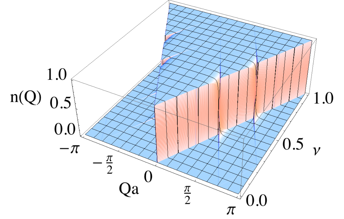
The fragmentation of the quasi-momentum distribution and the development of QP Fermi seas can be understood from first order perturbation theory. To first order in the momentum landscape becomes fragmented in six regions, shown in Fig.3 and given by:
| (12) | |||||
| (13) | |||||
| (14) | |||||
| (15) | |||||
| (16) | |||||
| (17) |
Where . The various regions are delineated by the edges of the QP Fermi seas, shown by white lines in Fig.3 and given in the space by :
| (18) |
The regions , and reflect the characteristic particle-hole symmetry in fermionic systems.
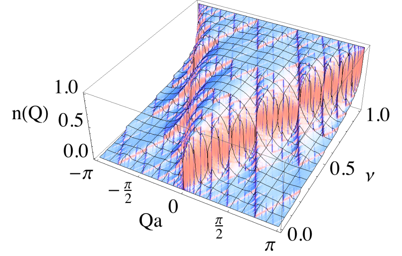
As disorder is increased, more quasi-Fermi seas become visible, and with the increase of they overlap in a complicated pattern. Exactly at criticality, , the pattern evolves into a fractal-like structure. Beyond the critical point, , the fragmented quasi-momentum distribution profile disappears and instead it becomes a smooth function of and . This behavior is summarized in Fig. 4 and the corresponding cross sections for fixed and are displayed in Fig. 5 and Fig. 6.
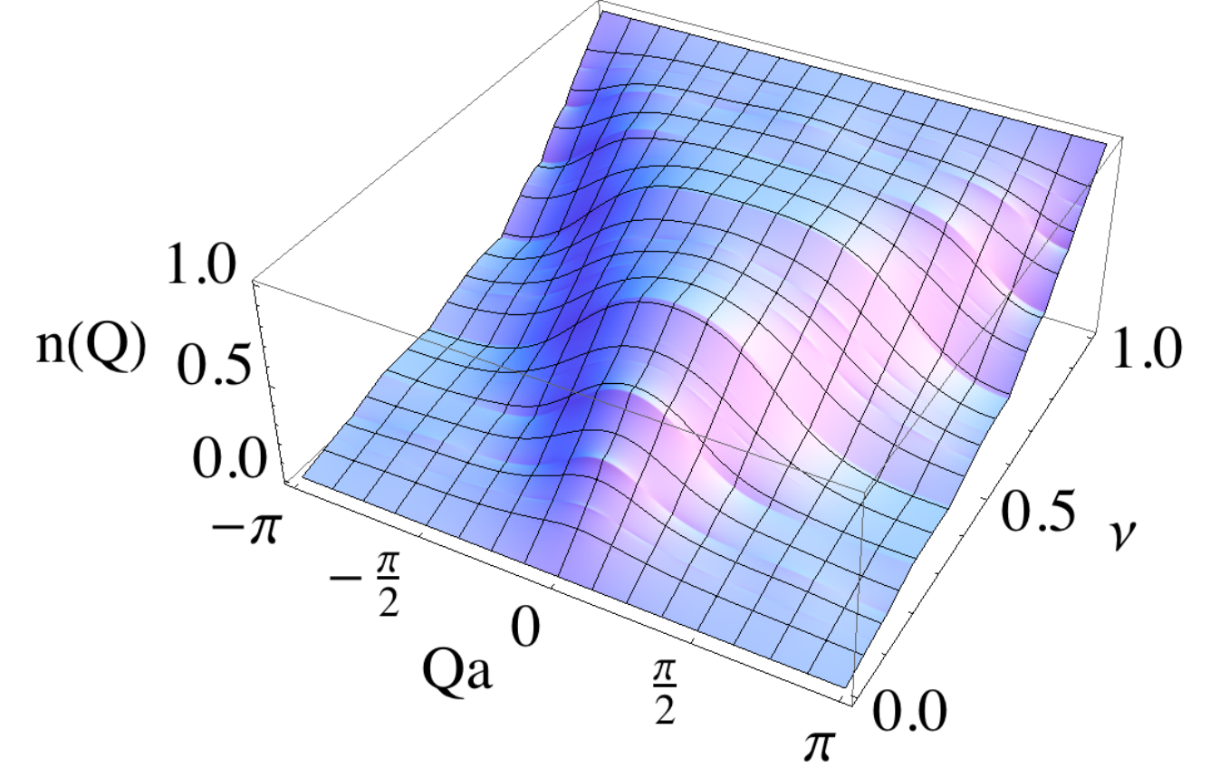
At irrational filling factors, however, the quasi-momentum distribution profile remains smooth regardless of the value of . The smoothness of the momentum distribution at these special filling factors can be understood using the same reasoning as the one used to understand the smooth character of the return map in position space in terms of non-degenerate perturbation theory. In this case, however, the states that are coupled are the ones localized at the quasi-momentum and , ( ).
The fragmentation of the Fermi sea in the regime, and the smooth profile in both the and band insulator phases are directly connected, via the self-duality property, to the discrete nature of the density return map in the localized phase, and its smooth character in the extended and band insulator phases.
An important point to emphasize again, which is crucial for possible experimental observation of the predicted behavior, is the insensitivity of the momentum distribution to variations of the phase . We demonstrate such insensitivity by noticing that the quasi-momentum distributions plotted in Fig.4 are actually averaged over many different values of . Hereafter all the plots in momentum space are always averaged over 50 random phases.


V.2 Arnold Tongues
Arnold tongues are mode-locked windows that characterize the periodic dynamics of iconic non-linear systems with competing periodicities. In the th century Christian Huyghens [25] noted that two clocks hanging back to back on a wall tend to synchronize their motion. In general coupled systems such as coupled pendula or pendula whose lengths vary periodically with time exhibit mode-locking [26]. As the parameters of a system are varied, it passes through regimes that are mode-locked and regimes which are not.
Arnold-like Tongues also appear in the QP fermionic momentum distribution, where they reflect the complex nature of the physics induced by the competing periodicities.


For , the Fermi distribution is a binary distribution with only two values . For finite and for generic filling factors, two windows of values centered around zero and unity become allowed whose width increases with as can be derived from a perturbative analysis. We call such windows QP tongues (See Fig. 7). Exactly at the onset of the metal-insulator transition the two distributions overlap, mimicking the Arnold tongue behavior. We have checked that the duality of the Harper equation allows one to observe the formation of analogous structures in position space. The absence of a metal insulator transition at the irrational filling factors at which the system is a band insulator is also signaled by the disappearance of the Arnold tongues at these fillings, as shown in Fig. 7(b).
V.3 Bifurcations
Bifurcations are common features observed in nonlinear dynamical systems, which occur when a small smooth change made to specific parameters (the bifurcation parameters) of the system causes a sudden ‘qualitative’ or topological change in its behavior. A series of bifurcations can lead the system from order to chaos.
The density distribution provides a nice manifestation of a single bifurcation with as a bifurcation parameter. When the density at the various Fibonacci sites is plotted as a function of , for an specific filling factor which depends on the value of , a bifurcation opens up at . In Fig. 8 the existence of a bifurcation at quarter filling () when is shown.
A qualitative understanding of the bifurcation can be gained by considering the two limiting regimes, and . In the weak coupling limit, , the local density is uniform and directly proportional to the filling factor . On the other hand, in the strong coupling limit, a given site remains empty or occupied depending upon whether the onsite potential is greater than or less than the Fermi energy.
Fibonacci sites have similar on-site energies which oscillate about (assuming and ) as:
These oscillations can be seen in Fig.13 in Appendix A.

Consequently, at the filling factor, , at which the Fermi energy matches (e.g. if then ) Eq. V.3 implies that as goes to infinity, even Fibonacci sites () become empty and odd Fibonacci sites () become occupied. This behavior combined with the monotonic increase of the density with in the weak coupling limit qualitatively explains the observed bifurcation.
The self-dual behavior described by Eq.11 implies the existence of the same bifurcation phenomena in quasi-momentum distribution but with the weak and the strong coupling limits reversed ( ).


When the local density is plotted for a generic lattice site as a function of and , the landscape shows a similar change in topology. In contrast to Fig. 8 where the filling factor is fixed but different curves corresponding to different Fibonacci sites are shown, in Fig. 9 the density at an specific lattice site is plotted but both the filling factor and disorder strength are varied. In this plot besides the large bifurcation there are smaller ones which cannot be explained by studying the two limiting cases. However, in momentum space they are qualitatively understood by considering cuts at a fixed as a function of . In these cuts the big jump at small can be identified with the edges of the main Fermi sea in the quasi-momentum profile and the smaller jumps correspond to edges of the quasi-Fermi seas.
V.4 Devil’s Staircases
A Devil’s staircase describes a self similar function , with a hierarchy of jumps or steps. In other words, exhibits more and more steps as one views the function at smaller and smaller length scale. The derivative of vanishes almost everywhere, meaning there exists a set of points of measure 0 such that for all outside it the derivative of exists and is zero.
Cold atom experiments may provide an opportunity to visualize devil’s staircases in the momentum-momentum correlations, namely the noise correlations.




Measurement of noise correlations is an example of Hanbury-Brown-Twiss interferometry (HBTI), which is sensitive to intrinsic quantum noise in intensity correlations. HBTI is emerging as one of the most important tools to provide information beyond that offered by standard momentum distribution-based characterization of phase coherence. The noise correlation pattern in 1D QP bosonic systems has been studied theoretically [27, 28, 29, 30] and has also been measured experimentally [22]. Here however we focus on the fermionic system.
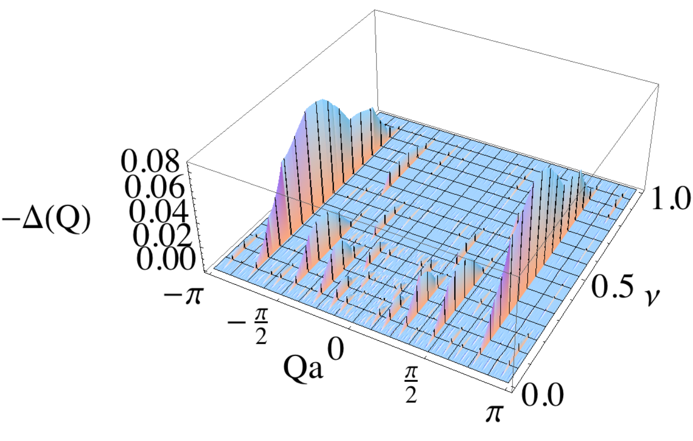
In the extended phase, noise correlations exhibit a series of plateaus as is varied, and the number of steps or plateaus increases as the strength of the disorder increases. The origin of this step-like structure with jumps occurring at the filling factors , can be understood from a perturbative argument as follows. For non-interacting fermions, for (See Fig.10), with being the Fourier transform of the single-particle eigenfunction. For , the overlap between any two different Fourier components is always zero as only the ground () state has a zero quasi-momentum component, i.e. . For small , first order perturbation theory yields a single step observed at , as only with is nonzero.
Quantitatively, the heights of the steps at for are given by:
| (22) |
Where () is the step height for () at filling factor . The minus sign implies a decrease in the noise as the filling factor increases. As increases, more and more steps are seen and can be explained using higher order perturbation theory. At criticality (see Figs.10-11), the steps acquire a hierarchical structure which resembles a devil’s staircase and which correlates with the fractal structure of the energy spectrum [23, 24]. In contrast to the momentum distribution, noise correlations do not show significant differences between the rational and irrational filling factors.
In the localized phase, , we see the smoothing of the step-structure and the noise correlation function tends towards a sinusoidal profile .
To emphasize the striking difference between the noise patterns in the extended and localized phases (the step-like vs smooth profile), in Fig. 12 we plot a measure of the gaps developed in as a function of .
VI Summary
We now summarize our key results:
- 1.
Extended-localized vs KAM-Cantori Phases
At the many-body level, the connection between the metal-insulator transition and the KAM-Cantori transition is signaled in the return map of the local density between nearest neighbor sites. For a given angle , the metallic phase with extended single particle wave functions exhibits a smooth return map. We identify this with the preserved invariant KAM tori in phase space at weak perturbations in the corresponding classical system. The localized phase displays a discrete return map, which we identify with the remaining tori or Cantori outside the perturbative regime. This behavior is shown in Fig.1. In addition, for the particular filling factors at which the system becomes a band insulator, the return map remains smooth for any value of (see Fig. 2).
Similar behavior can be observed in the corresponding momentum distribution return map. However, while the local density return map loses these characteristic features after averaging over , the momentum distribution return map remains almost unaffected. The robustness of the momentum return map to phase variations, is ideal for the experimental visualization of the metal-insulator vs KAM-Cantori connection in cold atoms.
- 2.
Quasi-fractal structures and Arnold Tongues
The introduction of weak disorder modifies the characteristic step-function Fermi-sea profile of the quasi-momentum distribution. Additional step-function structures centered at different reciprocal lattice vectors of the QP lattice appear for . We refer to those structures as the “quasi-Fermi seas”. With increasing and , the number and width of the various quasi-Fermi seas increase the fragmentation of the momentum distribution, turning it into a complex pattern. At the fragmentation becomes maximal and the momentum distribution evolves into a smooth profile as the system enters the localized phase (See figures 3-6). The overlap of the various quasi Fermi seas as one approaches criticality is reminiscent of the Arnold tongues overlap observed in non-linear systems, such as the circle map, as they enter the chaotic regime [31].
A more appropriate analogy of such behavior can be observed by considering the set of values taken by quasi-momentum distribution for a given filling factor. In the absence of disorder this distribution can only take the values 1 or 0, depending upon whether the quasi-momentum is greater or smaller than the Fermi quasi-momentum. As the strength of the quasi-periodic lattice increases, two distributions of values develop, centered around 0 and 1 respectively. Their width increases with increasing disorder and they overlap exactly at criticality (Fig.7).
- 3.
Bifurcations: The overlap between Arnold tongues at , can be linked, using the space-momentum duality transformation, to the appearance of a bifurcation in the density profile. The bifurcation occurs at a common but phase dependent filling for the various Fibonacci sites (Fig.8). At generic lattice sites, the filling factor at which the bifurcation takes place also depends on the lattice site under consideration and can be observed when the local density is plotted as a function of and (Fig.9).
- 4.
Systems with competing periodicities stand in between periodic and random systems. The richness and complexity underlying such systems have been studied extensively [18]. Ultracold atoms are emerging as a promising candidate to simulate a wide variety of physical phenomena. Here we have shown they offer opportunities to experimentally realize various paradigms of nonlinear dynamics.
Our focus here was on spin-polarized fermionic systems, since we wanted to look at the simplest consequences of many-body physics in disordered systems. However, Bose-Einstein condensed systems may also be used as tools for laboratory investigation of various predictions made for the quasi-periodic systems based on single-particle arguments [16]. For example, it might be possible to confirm the strong coupling universality prediction, which establishes that the ratio of the single particle density at two consecutive Fibonacci sites should be a universal number [32].
Acknowledgments A. M. Rey and S. Li acknowledge support from the NSF-PFC grant and NIST.
Appendix A Mapping from position to momentum space from self-duality relationship
Here we provide an example of the mapping between position coordinates and quasi-momentum coordinates which we use to link the quasimomentum-position observables. In the plot we highlight the Fibonacci sites. A small system size is used to make the visualization clearer.
Appendix B Perturbation Theory and Dimerized States
We begin our analysis with the Harper equation (2). For , the single particle wave functions are localized at individual lattice sites, and , where is defined by . When , we can get the single particle wave function through exact Diagonalization, or we can use the perturbation theory to obtain the approximate eigenvalues and eigenfunctions.
We focus first on the site . Assuming that , non-degenerate perturbation theory can be used, and the results are:
| (23) | |||||
| (24) | |||||
| (25) | |||||
| (26) | |||||
| (27) |
where , , are the zeroth, first and second order terms of the eigenvalue , with a similar meaning for and . Also, . So, up to first order of , .
For other sites that satisfy , non-degenerate perturbation theory doesn’t work and degenerate perturbation theory will be used. In that case, the zero order energies and eigenfunctions satisfy:
The above equations result in a pair of energies which we denote as and :
| (35) | |||||
| (36) |
where . The corresponding orthogonal eigenfunctions can be written as:
where , . We can choose () to be the greater (lesser) of and : , . From these results one can see that increases as increases. For example, when , and when , .

When , is comparable to and the states are localized at the same two neighboring sites. Hence, they will be referred as a pair of dimerized states ( The numerical results are shown in Fig.14 (a) ). The dimerized states are found by noticing that:
| (42) |
So for the points that satisfy , dimerized sites exist at and . Since , it is clear that we can construct the relation , where are indexes of increasing energy level, are indexes of sites’ positions and are indexes that we introduce for the convenience of discussion ( is the closest integer to ). Using this relation it can be shown that (we use here, since the exact expression for even and odd are slightly different). The relations of , and are plotted for the case of in Fig.14 (b).
As we discussed, the dimerized states satisfy:
| (43) |
Writing the above equation in terms of , we get:
The solutions are . Therefore,
| (44) | |||
| (45) |
which correspond to:
| (46) | |||
| (47) |
A detailed analysis shows that the band opens exactly at and regardless of being even or odd. This demonstrates, at perturbative level, the special behavior of the return map at irrational filling number or (See Fig.2).
In our calculations, we find out those with the lowest values of (avoiding double counting of in different pairs) and then apply to those points the perturbation theory we discussed above.
Based on the latter considerations it is possible to demonstrate that around or , there exists a sequence of paired states, exhibiting the following relationships as ,
with and . These states determine the properties of the system when the Fermi energy is close to the major gaps, i.e. or , and thus the main properties of the band insulator phases.
References
- [1] I. Bloch, J. Dalibard, and W. Zwerger, Rev. Mod. Phys. 80, 885 (2008).
- [2] M. Lewenstein et al., Advances in Physics 56, 243 (2007).
- [3] M. Greiner, O. Mandel, T. Esslinger, T. W. Hänsch, and I. Bloch, Nature 415, 39 (2002).
- [4] R. Jördens, N. Strohmaier, K. Gunther, H. Moritz, and T. Esslinger, Nature 455, 204 (2008).
- [5] U. Schneider et al., Science 322, 1520 (2008).
- [6] T. Kinoshita, T. Wenger, and D. S. Weiss, Science 305, 1125 (2004).
- [7] B. Paredes et al., Nature 429, 277 (2004).
- [8] S. R. Wilkinson, C. F. Bharucha, K. W. Madison, Q. Niu, and M. G. Raizen, Phys. Rev. Lett. 76, 4512 (1996).
- [9] F. L. Moore, J. C. Robinson, C. F. Bharucha, B. Sundaram, and M. G. Raizen, Phys. Rev. Lett. 75, 4598 (1995).
- [10] F. L. Moore, J. C. Robinson, C. Bharucha, P. E. Williams, and M. G. Raizen, Phys. Rev. Lett. 73, 2974 (1994).
- [11] L. Fallani, J. E. Lye, V. Guarrera, C. Fort, and M. Inguscio, Phys. Rev. Lett. 98, 130404 (2007).
- [12] D. R. Hofstadter, Phys. Rev. B 14, 2239 (1976).
- [13] M. Y. Azbel and M. Rubinstein, Phys. Rev. B 27, 6530 (1983).
- [14] A. N. Kolmogorov, Doklady Akad. Nauk SSSR 93, 763 (1953).
- [15] I. C. Percival, Journal of Physics A: Mathematical and General 12, L57 (1979).
- [16] K. Drese and M. Holthaus, Phys. Rev. Lett. 78, 2932 (1997).
- [17] S. Aubry and G. Andre, Proceedings of the Israel Physical Society, vol. 3 (Hilger, Bristol, 1979).
- [18] J. B. Sokoloff, Physics Reports 126, 189 (1985).
- [19] B. L. Tolra et al., Phys. Rev. Lett. 92, 190401 (2004).
- [20] C. D. Fertig et al., Phys. Rev. Lett. 94, 120403 (2005).
- [21] E. Altman, E. Demler, and M. D. Lukin, Phys. Rev. A 70, 013603 (2004).
- [22] V. Guarrera et al., Phys. Rev. Lett. 100, 250403 (2008).
- [23] S. Ostlund and R. Pandit, Phys. Rev. B 29, 1394 (1984).
- [24] S. Ostlund, R. Pandit, D. Rand, H. J. Schellnhuber, and E. D. Siggia, Phys. Rev. Lett. 50, 1873 (1983).
- [25] B. van der Pol, Stated in a footnote in , Philos. Mag. 3, 13 (1927).
- [26] V. I. Arnold, Mathematical methods of classical mechanics, Chapter V (Springer-Verlag, New York, 1994).
- [27] A. M. Rey, I. I. Satija, and C. W. Clark, New Journal of Physics 8, 155 (2006a).
- [28] A. M. Rey, I. I. Satija, and C. W. Clark, Phys. Rev. A 73, 063610 (2006b).
- [29] A. M. Rey, I. I. Satija, and C. W. Clark, Laser Physics 17, 205 (2007).
- [30] T. Roscilde, Phys. Rev. A 77, 063605 (2008).
- [31] E. Ott, Chaos in Dynamical Systems (Cambridge University Press, 1993).
- [32] J. A.Ketoja and I. I. Satija, Phys Rev Lett 75, 2762 (1995).