Single-file diffusion of a system of hardcore particles is a well-studied process that provides a basic description of transport, for example, in fast ion transport through channels [1, 2], in zeolites [3] and in superionic or organic conductors [4]. While their collective diffusion is like that of a set of independent particles, the diffusion of a tagged particle is known to be different - namely, its mean squared displacement (MSD) is proportional to $\sqrt{t}$ and its positions are Gaussian-distributed [5, 6, 7, 8, 9, 10, 11, 12]. It is an exactly solved problem in the case when the system consists of identical particles having the same diffusion constant. On the other hand, the case when their motion is characterized by a set of different diffusion constants is not readily amenable to an exact mathematical analysis. However, Ambjörnsson et al., [13, 14] have recently shown that the diffusion of a system consisting of just two hardcore particles with different diffusion constants on an unbounded (one dimensional) real line can be solved exactly; in particular, they have shown that the MSD of a tagged particle is proportional to $t$; they have also presented Monte Carlo evidence to show that it crosses over from diffusive ($\propto t$) to subdiffusive ($\propto\sqrt{t}$) behavior only if it is in the interior of a large system.

In this context, it is of interest to study the effect of constraining boundaries on the single-file diffusion of particles with different diffusion constants. Such boundary effects are relevant, for example, to understand the physical mechanism underlying the process of cell protrusion where polymerizing actin filaments push the cell membrane. The first physical description of the cell protrusion process was based on the Brownian Ratchet (BR) model [15, 16]. This is a one-dimensional two-particle representation for the filament-membrane system. In this model, the random diffusive motion of the cell membrane, represented as a Brownian obstacle, is rectified by the growing tip of a semi-rigid rod whose other end is fixed at the origin. Using the stationary distribution for the gap between the tip of the flexible rod and the obstacle, they could explain the experimentally observed load-velocity curves reasonably well.

In the two-particle model the membrane is represented by a single particle where the tension-induced correlations among the constituents of a two-dimensional flexible surface are neglected. In fact, a recent simulation study on two interacting random surfaces [17] representing the cell membrane and the actin cortex has indicated the importance of correlation [18]. The representation of a long semi-rigid actin filament by a single particle is reasonable as long as nucleation of new filaments near the leading edge of the protruding membrane is negligible. In this case, a single actin filament polymerizes and depolymerizes at its both ends such that shrinking and growing of its length would never lead to dissolvation. This assumption is justified based on the observation that in vivo the ATP-mediated (de)polymerization processes [19] can yield an effective ‘treadmilling’ [20] of a filament which, on average, depolymerizes only at its ‘minus’ end and polymerizes only at its ‘plus’ end at the same rate such that its average length remains constant. Therefore, the theoretical ansatz to consider only the growing plus end, which is located near the protruding edge of the cell membrane, and to model this by a single particle is reasonable. Furthermore, in the two-particle model the assumption is made that the whole filament is prohibited to perform large-scale thermal motion (e.g. diffusion). In vivo this immobility is mostly achieved by strong adhesive bonds connecting the filament via the cell membrane to the underlying substrate on which the cell crawls. Therefore, in the present two-particle model the immobility of the filament is presumed, and the only mechanism by which a cell can be moved is by pushing the leading front of the cell membrane (particle M) by the polymerizing plus end of a filament (drifting particle F).

We present an exact analysis of a two-particle system drift-diffusing on the positive real line in the case when particle F drifts and diffuses slowly towards particle M. The fluctuation in the position of the membrane particle M exhibits diffusive behavior at short, as well as at long times with an intermediate crossover-regime that is due to the onset of hardcore interaction between the particles. We show that this is in agreement with the results obtained from the set of Master equations that describe the stochastic evolution of the two-particle model. On the other hand, fluctuation in the position of the pushing ’filament’ particle F is diffusive without any such crossover behavior. The mean displacement of the Brownian particle M (’membrane’) crosses over from an initial diffusive behavior to an asymptotic drift behavior. For the sake of completeness we consider also the case of a repulsive boundary for F at the origin.

In the next section, we describe the one dimensional drift-diffusive motion of a pair of hardcore particles in terms of a set of hopping rates on a regular lattice and present a discussion of this process in the continuum limit. In section III, we compare the results obtained by solving the two-particle drift-diffusion equation with those obtained by numerically integrating the set of master equations, given in the Appendix, that describes the hopping process on a lattice.

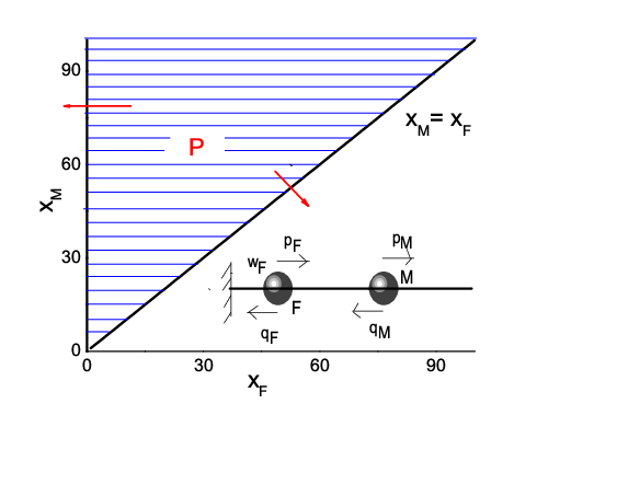
Let a pair of particles, labeled F and M, be at positions $n_{F}$ and $n_{M}$ respectively on a one dimensional lattice; hardcore interaction ensures that $n_{F}<n_{M}$ at all times, if that was the case at $t=0$. Equivalently, the distance of separation between these particles, $n\equiv(n_{M}-n_{F})$, satisfies the inequality $n\geq 1$ at all times. A schematic illustration of the model is shown in Fig.1.

Consider a discrete time process. At every instant of time, particle M moves one step to the right or to the left with a priori probability $p_{M}$ or $(1-p_{M})$ respectively; on the other hand, particle F may either move or stay put. Let $w_{F}$ be the probability that F will move at any given instant of time. Then, on the average, F moves just once during the period of time in which M has moved $1/w_{F}$ times. It is clear that $w_{F}$ also denotes the a priori probability that both F and M will move simultaneously at a given instant of time. Given that F moves, let it move one step to the right or to the left with a priori probability $p_{F}$ or $q_{F}\equiv(1-p_{F})$ respectively. Of course, with respect to the physico-biological situation, as described in the Introduction, the practically reasonable case is $q_{F}<p_{F}$, which implies $n_{F}>0$.

So, when both the particles jump simultaneously in the same direction, the separation distance, $n$, does not change; when they jump simultaneously in opposite directions, $n$ changes by $\pm 2$; on the other hand, when particle F does not jump, $n$ changes by $\pm 1$. Let $q_{0}^{\pm},q_{1}^{\pm},q_{2}^{\pm}$ denote the probabilities per unit time that the change in separation distance $\delta n=0,\pm 1,\pm 2$ respectively. They are given by

	$\displaystyle q_{0}^{+}$	$\displaystyle=$	$\displaystyle w_{F}p_{F}p_{M}$
	$\displaystyle q_{0}^{-}$	$\displaystyle=$	$\displaystyle w_{F}(1-p_{F})(1-p_{M})$
	$\displaystyle q_{1}^{+}$	$\displaystyle=$	$\displaystyle(1-w_{F})p_{M}$
	$\displaystyle q_{1}^{-}$	$\displaystyle=$	$\displaystyle(1-w_{F})(1-p_{M})$		(1)
	$\displaystyle q_{2}^{+}$	$\displaystyle=$	$\displaystyle w_{F}(1-p_{F})p_{M}$
	$\displaystyle q_{2}^{-}$	$\displaystyle=$	$\displaystyle w_{F}p_{F}(1-p_{M})$

and they all add up to unity.

The physically motivated constraint that the particles can only move on the positive real line, $n_{M}>n_{F}\geq 1$ (on a lattice), as well as the probability, $w_{F}$, for them to move simultaneously imply that we have different sets of Master Equations for the joint probability, $P(n_{F},n_{M};t)$ corresponding to the cases $n=1,2,\geq 3$ respectively (see, Appendix).

In the continuum description, the joint probability for the positions of the hardcore particles, $x_{F}$ and $x_{M}$, satisfies the following drift-diffusion equation,

	$\displaystyle\frac{\partial P(x_{F},x_{M};t)}{\partial t}$	$\displaystyle=$	$\displaystyle\left(D_{F}\frac{\partial^{2}P(x_{F},x_{M};t)}{\partial x_{F}^{2}}-\mu_{F}\frac{\partial P(x_{F},x_{M};t)}{\partial x_{F}}\right)+$		(2)
			$\displaystyle\left(D_{M}\frac{\partial^{2}P(x_{F},x_{M};t)}{\partial x_{M}^{2}}-\mu_{M}\frac{\partial P(x_{F},x_{M};t)}{\partial x_{M}}\right)$

which is, in fact, the continuum version of the unrestricted Master Equation, Eq( Appendix - Master Equations for the two-particle system
). Hardcore interaction between the particles constrained to be on the positive real line implies that $x_{M}>x_{F}\geq 0$ at all times. In our model, particle M is purely diffusive whereas particle F can drift as well. Therefore, as shown in Appendix (f), the corresponding diffusion and drift coefficients are given by,

	$\displaystyle D_{F}$	$\displaystyle=$	$\displaystyle\frac{1}{2}(q_{2}^{+}+q_{2}^{-}+q_{0}^{+}+q_{0}^{-})$
		$\displaystyle=$	$\displaystyle\left(\frac{1}{2}w_{F}(1-w_{F})+2w_{F}^{2}p_{F}(1-p_{F})\right)\ \approx\frac{1}{2}w_{F}\quad\mbox{($w_{F}$ small)}$
	$\displaystyle\mu_{F}$	$\displaystyle=$	$\displaystyle-q_{2}^{+}+q_{2}^{-}+q_{0}^{+}-q_{0}^{-}=w_{F}(2p_{F}-1)$
	$\displaystyle D_{M}$	$\displaystyle=$	$\displaystyle\frac{1}{2}(q_{2}^{+}+q_{2}^{-}+q_{1}^{+}+q_{1}^{-}+q_{0}^{+}+q_{0}^{-})=\frac{1}{2}$
	$\displaystyle\mu_{M}$	$\displaystyle=$	$\displaystyle q_{2}^{+}-q_{2}^{-}+q_{1}^{+}-q_{1}^{-}+q_{0}^{+}-q_{0}^{-}=0$

The initial condition for this problem could be specified by the joint probability distribution,

$$P(x_{F},x_{M};t=0)=\delta(x_{F}-x_{F}^{0})\delta(x_{M}-x_{M}^{0})$$

(4)

where $\delta(x)$ is the Dirac delta function. The first boundary condition,

$$\left(D_{M}\frac{\partial P(x_{F},x_{M};t)}{\partial x_{M}}-D_{F}\frac{\partial P(x_{F},x_{M};t)}{\partial x_{F}}\right)_{x_{F}=x_{M}}=\left[(\mu_{M}-\mu_{F})P(x_{F},x_{M};t)\right]_{x_{F}=x_{M}}$$

(5)

expresses the fact that the particles cannot pass each other ($x_{F}<x_{M}$). The second boundary condition,

$$\left(D_{F}\frac{\partial P(x_{F},x_{M};t)}{\partial x_{F}}-\mu_{F}P(x_{F},x_{M};t)\right)_{x_{F}=0}=0$$

(6)

ensures that there is no current across the boundary at $x_{F}=0$. These two boundaries define a wedge as the domain for the joint distribution $P(x_{F},x_{M};t)$. The question is whether a separable solution to Eq.(2) can be found. We first transform the variables, $\{x_{F},x_{M}\}$, into a pair of ’collective’ variables, say $\{x,r\}$.

Inter-particle separation, $r\equiv x_{M}-x_{F}$, could be fixed as one of the new variables. For the other variable, we set $x=c_{M}x_{M}+c_{F}x_{F}$ and try to fix the dimensionless constants, $c_{M}$ and $c_{F}$, by requiring that the transformed drift-diffusion equation also has the same form as Eq.(2). This requirement leads to the condition that the coefficient of ${\partial^{2}P(x,r;t)}/{\partial x}{\partial r}$ vanishes:

$$D_{M}c_{M}-D_{F}c_{F}=0,$$

(7)

This implies that

$$c_{M}\sqrt{\frac{D_{M}}{D_{F}}}=c_{F}\sqrt{\frac{D_{F}}{D_{M}}}=c$$

(8)

where $c$ is an arbitrary constant. We set $c=1/2$ so that $x$ will be the position of the center-of-mass of the system when the particles are of the same mass and have the same value for their diffusion constants ($D_{M}=D_{F}$). In general, $x$ is not the center-of-mass coordinate because the equality, $c_{M}+c_{F}=1$, will be satisfied only when the particles have the same mass and also when $D_{M}=D_{F}$. Nevertheless, with the choice $c=1/2$, we have the transformation,

	$\displaystyle x$	$\displaystyle=$	$\displaystyle\frac{1}{2}\left(\sqrt{\frac{D_{M}}{D_{F}}}\ x_{F}+\sqrt{\frac{D_{F}}{D_{M}}}\ x_{M}\right)$
	$\displaystyle r$	$\displaystyle=$	$\displaystyle x_{M}-x_{F}$

under which Eq.(2) becomes

$$\frac{\partial P(x,r;t)}{\partial t}=\left(D_{x}\frac{\partial^{2}P(x,r;t)}{\partial x^{2}}-\mu_{x}\frac{\partial P(x,r;t)}{\partial x}\right)+\left(D_{r}\frac{\partial^{2}P(x,r;t)}{\partial r^{2}}+\mu_{r}\frac{\partial P(x,r;t)}{\partial r}\right)$$

(10)

with the initial condition,

$$P(x,r;t=0)=\left(\frac{D_{F}+D_{M}}{2\sqrt{D_{F}D_{M}}}\right)\ \delta(x-x^{0})\ \delta(r-r^{0})$$

(11)

where

	$\displaystyle D_{x}$	$\displaystyle=$	$\displaystyle(D_{M}+D_{F})/4$
	$\displaystyle D_{r}$	$\displaystyle=$	$\displaystyle D_{M}+D_{F}$
	$\displaystyle\mu_{x}$	$\displaystyle=$	$\displaystyle\frac{1}{2}\left(\sqrt{\frac{D_{M}}{D_{F}}}\ \mu_{F}+\sqrt{\frac{D_{F}}{D_{M}}}\ \mu_{M}\right)$		(12)
	$\displaystyle\mu_{r}$	$\displaystyle=$	$\displaystyle\mu_{F}-\mu_{M}$
	$\displaystyle x^{0}$	$\displaystyle=$	$\displaystyle\frac{1}{2}\left(\sqrt{\frac{D_{M}}{D_{F}}}\ x_{F}^{0}+\sqrt{\frac{D_{F}}{D_{M}}}\ x_{M}^{0}\right)$
	$\displaystyle r^{0}$	$\displaystyle=$	$\displaystyle x_{M}^{0}-x_{F}^{0}$

The boundary condition, Eq.(5), that ensures hardcore repulsion between the particles now transforms into the following condition,

$$\left[D_{r}\frac{\partial P}{\partial r}+\mu_{r}P\right]_{r=0}=0$$

(13)

which is the reflecting boundary condition at $r=0$ (i.e., $x_{F}=x_{M}$) for the above drift-diffusion equation for $P(x,r;t)$. The other boundary condition, Eq.(6), transforms into

$$\left[\frac{1}{2}\sqrt{D_{M}D_{F}}\ \frac{\partial P}{\partial x}-D_{F}\frac{\partial P}{\partial r}-\mu_{F}P\right]_{x=\frac{1}{2}\sqrt{\frac{D_{F}}{D_{M}}}\ r}=0$$

(14)

It is clear that the wedge in $\{x_{F},x_{M}\}$-space has transformed into a wedge in the $\{x,r\}$-space. Moreover, the above boundary condition implies that separable solution to Eq.(10) is not possible in the transformed space.

A. No reflecting boundary at $x_{F}=0$:

One way to ensure separable solution to Eq.(10) is to ignore the boundary condition, Eq.(6), and hence Eq.(14). This amounts to assuming that the growing filament does not degrade to a monomer in any arbitrary time span of interest; so, particle F moves freely as long as it is to the left of particle M. In this case, we may now try a product solution to Eq.(10) of the form,

$$P(x,r;t)=\left(\frac{D_{F}+D_{M}}{2\sqrt{D_{F}D_{M}}}\right)P(x;t)P(r;t)$$

(15)

so that $P(x;t)$ and $P(r;t)$ satisfy the equations:

	$\displaystyle\frac{\partial P(x;t)}{\partial t}$	$\displaystyle=$	$\displaystyle D_{x}\frac{\partial^{2}P(x;t)}{\partial x^{2}}-\mu_{x}\frac{\partial P(x;t)}{\partial x}$
	$\displaystyle\frac{\partial P(r;t)}{\partial t}$	$\displaystyle=$	$\displaystyle D_{r}\frac{\partial^{2}P(r;t)}{\partial r^{2}}+\mu_{r}\frac{\partial P(r;t)}{\partial r}$

The first one is a free-boundary equation with the initial condition, $P(x;t=0)=\delta(x-x^{0})$, whereas the second one, with the initial condition $P(r;t=0)=\delta(r-r^{0})$, is subject to the boundary condition given by Eq.(13). Solutions can be written down immediately [21]:

	$\displaystyle P(x;t)$	$\displaystyle=$	$\displaystyle g\left(\frac{x-x^{0}-\mu_{x}t}{\sqrt{4D_{x}t}}\right)$
	$\displaystyle P(r;t)$	$\displaystyle=$	$\displaystyle g\left(\frac{r-r^{0}+\mu_{r}t}{\sqrt{4D_{r}t}}\right)+e^{\mu_{r}r^{0}/D_{r}}g\left(\frac{r+r^{0}+\mu_{r}t}{\sqrt{4D_{r}t}}\right)+$
			$\displaystyle\qquad\qquad\qquad\frac{\mu_{r}}{D_{r}}e^{-\mu_{r}r/D_{r}}\int_{y=r^{0}}^{\infty}g\left(\frac{y+r-\mu_{r}t}{\sqrt{4D_{r}t}}\right)dy$

where $g(\xi/\sigma)$ is the normalized gaussian function given by

$$g(\xi/\sigma)=\frac{1}{\sqrt{\pi\sigma^{2}}}\ e^{-\xi^{2}/\sigma^{2}}$$

(18)

The distribution $P(r;t)$ will become asymptotically stationary when $\mu_{r}>0$; this implies the condition $w_{F}(2p_{F}-1)>(2p_{M}-1)$ which is to say that the effective rightward drift of particle F should be more than that of particle M. It is clear from the definition, Eq.(2  Two hardcore particles on a 1d lattice:

Drift-Diffusion equation for the joint probability distribution), that stationary value for $\langle r\rangle$ does not imply stationary values for $\langle x_{M}\rangle$ and $\langle x_{F}\rangle$.

In the Brownian Ratchet model [15, 16] a reflecting boundary at the origin is introduced in order to provide a load which prohibits backflow of the actin filament. In this model the (de)polymerizing filament is represented by a rod where the plus end can (de)polymerize and the minus end of the filament is fixed at the origin. Since particle F represents the plus end of the rod, which has to be of nonzero length, we have a reflecting boundary for particle F at the origin.

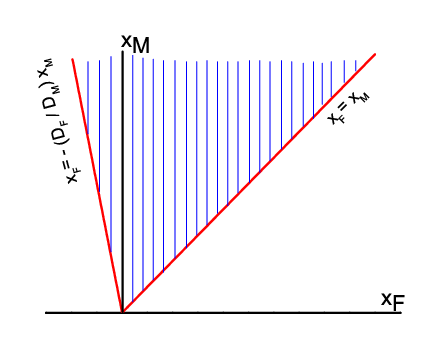
This reflecting boundary at $x_{F}=0$ transforms into the boundary condition Eq.(14), which rules out a separable form for $P(x,r;t)$. On the other hand, a separable solution to Eq.(10) can still be obtained if we arbitrarily impose the following boundary condition at $x=0$:

$$\left[D_{x}\frac{\partial P(x;t)}{\partial x}-\mu_{x}P(x;t)\right]_{x=0}=0$$

(19)

From the definition, Eq.(2  Two hardcore particles on a 1d lattice:

Drift-Diffusion equation for the joint probability distribution), we see that $x=0$ implies $x_{F}=-(D_{F}/D_{M})x_{M}$; hence the domain for the joint distribution, $P(x_{F},x_{M};t)$, is the wedge schematically shown in Fig.3. It is unphysical if we insist that particle F represents the tip of a polymer rod; yet, for small $w_{F}$ (by definition, Eq.(2  Two hardcore particles on a 1d lattice:

Drift-Diffusion equation for the joint probability distribution), $(D_{F}/D_{M})\approx w_{F}$), we may expect to have an approximate solution to the model.

Assuming separable form for $P(x,r;t)$ (Eq.(15)), the above boundary condition at $x=0$ leads to the solution, [21]

	$\displaystyle P(x;t)$	$\displaystyle=$	$\displaystyle g\left(\frac{x-x^{0}-\mu_{x}t}{\sqrt{4D_{x}t}}\right)+e^{-\mu_{x}x^{0}/D_{x}}g\left(\frac{x-x^{0}-\mu_{x}t}{\sqrt{4D_{x}t}}\right)-$		(20)
			$\displaystyle\qquad\qquad\qquad\frac{\mu_{x}}{D_{x}}e^{\mu_{x}x/D_{x}}\int_{y=x^{0}}^{\infty}g\left(\frac{y+x+\mu_{x}t}{\sqrt{4D_{x}t}}\right)dy$

The distributions, $P(x;t)$, will become asymptotically stationary when $\mu_{x}<0$. From the definitions, Eqs.(2  Two hardcore particles on a 1d lattice:

Drift-Diffusion equation for the joint probability distribution,12), we see that $\mu_{x}=w_{F}(p_{M}+p_{F}-1)$ and so $\mu_{x}<0$ implies the condition $p_{F}<q_{M}$. This will be realized when the leftward drift of particle M is more than the rightward drift of particle F. Interestingly, stationary value for $\langle x\rangle$ implies, by definition Eq.(2  Two hardcore particles on a 1d lattice:

Drift-Diffusion equation for the joint probability distribution), stationary values for $\langle x_{M}\rangle$ and $\langle x_{F}\rangle$ also, which in turn implies stationary value for $\langle r\rangle$. Hence, the condition $\mu_{x}<0$ is enough to ensure that the joint probability distribution, $P(x,r;t)$, becomes stationary.

Transforming back to the variables, $x_{F}$ and $x_{M}$, with appropriate Jacobian prefactor, the above solutions for $P(x;t)$ and $P(r;t)$ lead to the joint distribution $P(x_{F},x_{M};t)$ and hence to the tagged particle distributions:

	$\displaystyle P(x_{F};t)$	$\displaystyle=$	$\displaystyle\int_{x_{F}^{+}}^{\infty}dx_{M}P(x_{F},x_{M};t)$
	$\displaystyle P(x_{M};t)$	$\displaystyle=$	$\displaystyle\int_{-\infty}^{x_{M}^{-}}dx_{F}P(x_{F},x_{M};t)$

The upper limit $x_{M}^{-}$ suggests that $x_{F}$ may be arbitrarily close but never equal to $x_{M}$; similarly, the lower limit $x_{F}^{+}$ suggests that $x_{M}$ may be arbitrarily close but never equal to $x_{F}$. The Mean Squared Displacement (MSD) of a tagged particle, $\sigma_{M,F}^{2}$, may then be obtained from its corresponding distribution.

Stationarity for the distribution $P(r;t)$ in Eq.(2  Two hardcore particles on a 1d lattice:

Drift-Diffusion equation for the joint probability distribution) is ensured by the condition $\mu_{r}>0$ which, from Eqs.(2  Two hardcore particles on a 1d lattice:

Drift-Diffusion equation for the joint probability distribution,12), implies $w_{F}(2p_{F}-1)>(2p_{M}-1)$. In this case, the asymptotic stationary form of $P(r)$ is given by

$$P(r)=P(r;t\to\infty)=\frac{\mu_{r}}{D_{r}}\ e^{-\mu_{r}r/D_{r}}$$

(22)

which leads to the asymptotically stationary values for the moments:

	$\displaystyle\langle r\rangle_{t\to\infty}$	$\displaystyle=$	$\displaystyle\frac{D_{r}}{\mu_{r}}$
	$\displaystyle\langle r^{2}\rangle_{t\to\infty}$	$\displaystyle=$	$\displaystyle 2\left(\frac{D_{r}}{\mu_{r}}\right)^{2}$

Initial time-dependence of these moments and their approach to these stationary values can be obtained from their full forms:

	$\displaystyle\langle r\rangle$	$\displaystyle=$	$\displaystyle\frac{D_{r}}{2\mu_{r}}\mbox{erfc}(r^{0-})+\frac{1}{2}(r^{0}-\mu_{r}t)\mbox{erfc}(-r^{0-})-$		(24)
			$\displaystyle\frac{D_{r}}{2\mu_{r}}\ e^{\mu_{r}r^{0}/D_{r}}\mbox{erfc}(r^{0+})+\sqrt{\frac{D_{r}t}{\pi}}e^{-(r^{0-})^{2}}$

	$\displaystyle\langle r^{2}\rangle$	$\displaystyle=$	$\displaystyle\left(\frac{D_{r}}{\mu_{r}}\right)^{2}\left[(\mbox{erfc}(r^{0-})-e^{\mu_{r}r^{0}/D_{r}}\mbox{erfc}(r^{0+})\right]-$		(25)
			$\displaystyle\frac{2D_{r}}{\mu_{r}}\left[\sqrt{\frac{D_{r}t}{\pi}}e^{-(r^{0-})^{2}}-\frac{1}{2}(r^{0}+\mu_{r}t)\mbox{erfc}(r^{0+})\right]+$
			$\displaystyle\frac{1}{2}\left[(\mu_{r}t)^{2}+2(D_{r}-\mu_{r}r^{0})t+(r^{0})^{2}\right]\mbox{erfc}(-r^{0-})+(r^{0}-\mu_{r}t)\sqrt{\frac{D_{r}t}{\pi}}e^{-(r^{0-)^{2}}}$

where we have the definitions,

	$\displaystyle r^{0+}$	$\displaystyle=$	$\displaystyle\frac{r^{0}+\mu_{r}t}{\sqrt{4D_{r}t}}$
	$\displaystyle r^{0-}$	$\displaystyle=$	$\displaystyle\frac{r^{0}-\mu_{r}t}{\sqrt{4D_{r}t}}$		(26)
	$\displaystyle\mbox{erfc}(x)$	$\displaystyle=$	$\displaystyle 1-\frac{2}{\sqrt{\pi}}\int_{0}^{x}e^{-y^{2}}dy$

The ’early’ time behavior ($t<r^{0}/\mu_{r}$) of the moments can be guessed by recognizing that $r^{0\pm}\sim r^{0}/\sqrt{4D_{r}t}$ is large and therefore, in the limiting case $\mu_{r}\to 0$ for example, the average separation $\langle r\rangle$ increases proportional to $\sqrt{t}$; larger the value of $\mu_{r}$, shorter will be the growth regime $\langle r\rangle\propto\sqrt{t}$ because it will attain its stationary value $D_{r}/\mu_{r}$ faster.

It will be interesting to compare these results with those obtained by numerically integrating the Master equations, Eqs. 38), given in the Appendix (e). We have presented in Fig.4(a) the distributions of separation-distance obtained by numerically integrating these equations for 133 and 3398 time steps respectively; the distribution is clearly exponential at $t=3398$ - namely, $P(r)\sim 0.1e^{-0.096r}$ suggesting that the average value $\langle r\rangle\sim 10.42$. For the parameters used in the computation, the stationary value of $\langle r\rangle$ should be $D_{r}/\mu_{r}=(1+w_{F})/2w_{F}=10.5$ according to Eq.(3  Results and Discussions
). Even the normalizing constant ($\sim 0.1$) obtained from the Master equations is close to the expected value of $\mu_{r}/D_{r}\sim 0.095$.

In fact, the diffusion coefficient, $D_{n}$, obtained from Eq.(38) in the continuum limit for the case $n\geq 3$ is equal to $D_{r}$ (Eq.(12) for $p_{M}=1/2$ and $w_{F}$ small; but, $\mu_{n}=\mu_{r}$ whatever be the value of $p_{M}$.

The small difference in the approach of $\langle r\rangle$ to its stationary value, observed in Fig.4(b) for the case $p_{M}=1/2$, implies that the distribution obtained by integrating the Master Equations is not completely stationary even after 3398 time steps for the lattice size chosen; moreover, finite size effects could make slight differences because of the need to have boundary equations for $n=L$ and $n=(L-1)$ similar to what we have for $n=1$ and $n=2$.

In the case when there is no reflecting boundary at $x_{F}=0$, the variable $x$ is unbounded and hence its distribution $P(x;t)$ is a gaussian (Eq.(2  Two hardcore particles on a 1d lattice:

Drift-Diffusion equation for the joint probability distribution)) with the following moments:

	$\displaystyle\langle x\rangle$	$\displaystyle=$	$\displaystyle x_{0}+\mu_{x}t$
	$\displaystyle\langle x^{2}\rangle$	$\displaystyle=$	$\displaystyle 2D_{x}t+(x_{0}+\mu_{x}t)^{2}$

On the other hand, when the variable $x$ is constrained to be positive, its distribution $P(x;t)$ is given by Eq.(20). The corresponding moments can be obtained from Eqs.(24) and (25) by making the following replacements:

	$\displaystyle r\leftrightarrow x$	;	$\displaystyle\qquad r^{0}\leftrightarrow x^{0}$
	$\displaystyle\mu_{r}\leftrightarrow-\mu_{x}$	;	$\displaystyle\qquad D_{r}\leftrightarrow D_{x}$		(28)
	$\displaystyle r^{0-}\leftrightarrow x^{0+}$	;	$\displaystyle\qquad r^{0+}\leftrightarrow x^{0-}$

The moments have the following asymptotic behavior ($\mu_{x}>0$):

	$\displaystyle\langle x\rangle_{t\to\infty}$	$\displaystyle=$	$\displaystyle\mu_{x}t+\left(x^{0}+\frac{D_{x}}{\mu_{x}}\ e^{-\mu_{x}x^{0}/D_{x}}\right)$
	$\displaystyle\langle x^{2}\rangle_{t\to\infty}$	$\displaystyle=$	$\displaystyle(\mu_{x}t)^{2}+2(D_{x}+\mu_{x}x^{0}+D_{x}e^{-\mu_{x}x^{0}/D_{x}})t+\mbox{const.}$

It is tempting to see how the mean-squared fluctuation in the position of a tagged particle, say M, would be related to those corresponding to the variables, $r$ and $x$, given the fact that the transformation $(x_{M},x_{F})\longleftrightarrow(r,x)$ is one-to-one. Quite surprisingly, the following ansatz,

$$\sigma_{M}^{2}\equiv\langle x_{M}^{2}\rangle-\langle x_{M}\rangle^{2}=\frac{4D_{M}D_{F}}{(D_{M}+D_{F})^{2}}\left(\sigma_{x}^{2}+\frac{1}{4}\frac{D_{M}}{D_{F}}\ \sigma_{r}^{2}\right)$$

(30)

with $\sigma_{x,\ r}^{2}$ calculated using the distributions, $P(x;t)$ and $P(r;t)$ given by Eq.(20) and Eq.(2  Two hardcore particles on a 1d lattice:

Drift-Diffusion equation for the joint probability distribution) respectively, leads to a striking agreement with those obtained from the Master equations.

In Fig.5(a), we have presented $\sigma_{M}$ obtained by using the above ansatz for the case when we have a reflecting boundary at $x=0$ (continuous line A) as well as from the Master Equations (open circles). The parameters are $w_{F}=0.05;p_{F}=1;p_{M}=1/2$ and the agreement is quite good. In the same figure, continuous line B represents $\sigma_{M}$ obtained using the above ansatz but for the case when there is no reflecting boundary at $x_{F}=0$. Its long-time deviation from both the case corresponding to a reflecting boundary at $x=0$ (continuous line A) and the Master eqns.(open circles) indicates that it does not represent the basic phenomenology of the Master eqns.

On the other hand, a similar ansatz for the average positions

$$\langle x_{M}\rangle=\frac{2\sqrt{D_{M}D_{F}}}{D_{M}+D_{F}}\left(\langle x\rangle+\frac{1}{2}\sqrt{\frac{D_{M}}{D_{F}}}\ \langle r\rangle\right)$$

(31)

does not lead to such a good agreement with what we obtain from the Master Equations at early times. However, it leads to qualitatively similar asymptotic behaviors - namely, the drift velocities are proportional to each other, the proportionality constant being $w_{F}$-dependent. For example, in (Fig.5(b)), the average velocity of particle M obtained from the Master Equations (open circles) is presented along with that obtained using the ansatz Eq.(31) (line M). It is quite clear that their asymptotic drift velocities are just proportional to each other even though their early time behaviors are different. Line F in the figure is the velocity of particle F obtained by using the above ansatz. While it takes some time, say $\tau_{M}^{d}$ that depends on $w_{F}$ and $p_{F}$, for M to start drifting with constant velocity, F starts drifting almost from the beginning.

In Fig.6(a), we have presented $\sigma_{M}$ obtained by using the above ansatz for the case when we have a reflecting boundary at $x=0$ but with $w_{F}=0.1$ (continuous line); the agreement with the Master Equations’ data (open circles) is reasonably good. On the other hand, in the case $w_{F}=0.2$ presented in Fig.6(b), there is no agreement between the analytically computed data (continuous line) and those obtained from the Master equations(open circles). This demonstrates, as mentioned earlier, that results obtained with an unphysical reflecting boundary at $x=0$ may agree with those obtained with the physically meaningful reflecting boundary at $x_{F}=0$ for small values of $w_{F}$ (namely, $w_{F}\leq 0.1$ with $p_{F}=1$ and $p_{M}=1/2$).

In Fig.7(a), we have shown how the crossover-behavior of $\sigma_{M}$ contrasts with the monotonously increasing behavior of $\sigma_{F}$. It is only when particle F has no effective drift towards particle M that such a crossover is non-existent (see Fig.7(b)); larger the effective drift, sooner is the crossover seen. It remains to be answered whether it is due to the reflecting boundary at the origin.

We have shown in Fig.8 the fluctuation in the position of M for the cases, with as well as without a reflecting boundary at $x=0$. The parameters used are mentioned in the caption. It is clear that the crossover becomes more pronounced and shifted to later times in the presence of a reflecting boundary than in its absence. In fact, the crossover is due to the smaller diffusivity of particle F than that of particle M ($D_{F}<D_{M}$). The effective drift of particle F leads to the saturation of the average separation-distance.

It is appropriate, at this juncture, to compare this model with the standard BR model [15, 16]. The ratchet mechanism, in the BR model, is due to a monomer squeezing itself in the gap between the filament-tip and the barrier particle (i.e., the membrane). The resulting growth of the filament-rod is impeded by the inward (forced) drift of the barrier particle. This leads to a steady state in which the average gap betwen the filament tip and the barrier remains constant. The average ratchet velocity, in the steady state, is proportional to the net polymerization rate of the filament and is given by

$$v_{BR}=\delta\left(\alpha\ \mbox{exp}\left[-\frac{Df}{k_{B}T}\right]-\beta\right)$$

(32)

where $\alpha$ and $\beta$ are the polymerization and depolymerization rates respectively; $D$ is the diffusion constant of the barrier particle, which drifts towards the filament-tip under the influence of the dimensionless force, $f/k_{B}T$; and, $\delta$ is the size of the intercalating monomer.

In our model, the BR-parameters ($\delta$, $\alpha$, $\beta$, $D$ and $f/k_{B}T$) are all lumped into the parameters $w_{F}$ and $p_{F}$ so that the drift coefficient $\mu_{F}$, defined in Eq.(2  Two hardcore particles on a 1d lattice:

Drift-Diffusion equation for the joint probability distribution), is equivalent to the ratchet velocity, $v_{BR}$:

$$\mu_{F}\equiv v_{BR}$$

(33)

Stationarity for the gap distribution is ensured by the condition $\mu_{F}>\mu_{M}$, which is equivalent to the condition $w_{F}>0$ in the case when $\mu_{M}=0$ and $p_{F}=1$ (see also, Fig.4(b)). In other words, the effect of the load-force and the consequent inward drift of the barrier particle in the BR model is mimicked in our model by the parameter $w_{F}>0$, which also tunes the steady state value of the average gap, $\langle r\rangle$ (Eq.(3  Results and Discussions
). So, our model can be thought of as a variant of the BR model [15, 16] that addresses the positional fluctuations of the particles M and F as well.

In summary, we have discussed a two-particle model of cell protrusion namely, a system of two hardcore particles diffusing with different rates. The Brownian particle, labeled M, experiences a random hardcore ’push’ by another particle, labeled F; M may be referred to as the ’driven’ particle.

We have solved the equations in the case when the drift-diffusion of particle F is small and obtained exact expressions for the tagged particle moments. Physically, this corresponds to the situation when the effective drift of particle F towards particle M is small. Since particle M represents a ’membrane’, fluctuations in its position is of interest when it is being ’driven’ by another particle F. Computed from the exact solutions (and using the ansatz Eq.(30)), our theory exhibits a crossover from an initial diffusive behavior to an asymptotic diffusive behavior. The existence and duration of the crossover regime depends on the diffusivities of the particles. It compares very well with the fluctuation data obtained by numerically integrating a complete set of Master equations that describe the stochastic dynamics of this model. Asymptotic diffusion of a tagged particle is, of course, expected for a finite system.

Let $P(n_{F},n_{M};t)$ denote the probability that, at a given instant of time $t$, the particles F and M are at positions $n_{F}$ and $n_{M}$ respectively. The distance between them, $n=n_{M}-n_{F}$, satisfies the inequality $n\geq 1$ at all times; the jump probabilities per unit time, $\{q\}$, are defined in section 2, Eq.(1).

	$\displaystyle\frac{\partial P(1,2;t)}{\partial t}$	$\displaystyle=$	$\displaystyle q_{1}^{-}P(1,3;t)+q_{0}^{-}P(2,3;t)-(q_{1}^{+}+q_{0}^{+})P(1,2;t)$
	$\displaystyle\frac{\partial P(n_{F},n_{F}+1;t)}{\partial t}$	$\displaystyle=$	$\displaystyle q_{2}^{-}P(n_{F}-1,n_{F}+2;t)+q_{1}^{-}P(n_{F},n_{F}+2;t)+$
			$\displaystyle q_{0}^{-}P(n_{F}+1,n_{F}+2;t)+q_{0}^{+}P(n_{F}-1,n_{F};t)-$
			$\displaystyle(q_{2}^{+}+q_{1}^{+}+q_{0}^{+}+q_{0}^{-})P(n_{F},n_{F}+1;t);\quad(n_{F}\geq 2)$

	$\displaystyle\frac{\partial P(1,3;t)}{\partial t}$	$\displaystyle=$	$\displaystyle q_{1}^{-}P(1,4;t)+q_{1}^{+}P(1,2;t)+q_{0}^{-}P(2,4;t)-$
			$\displaystyle(q_{1}^{+}+q_{1}^{-}+q_{0}^{+})P(1,3;t)$
	$\displaystyle\frac{\partial P(n_{F},n_{F}+2;t)}{\partial t}$	$\displaystyle=$	$\displaystyle q_{2}^{-}P(n_{F}-1,n_{F}+3;t)+q_{1}^{-}P(n_{F},n_{F}+3;t)+q_{1}^{+}P(n_{F},n_{F}+1;t)+$
			$\displaystyle q_{0}^{-}P(n_{F}+1,n_{F}+3;t)+q_{0}^{+}P(n_{F}-1,n_{F}+1;t)-$
			$\displaystyle(q_{2}^{+}+q_{1}^{+}+q_{1}^{-}+q_{0}^{+}+q_{0}^{-})P(n_{F},n_{F}+2;t);\quad(n_{F}\geq 2)$

	$\displaystyle\frac{\partial P(1,1+n;t)}{\partial t}$	$\displaystyle=$	$\displaystyle q_{2}^{+}P(2,n;t)+q_{1}^{-}P(1,2+n;t)+$
			$\displaystyle q_{1}^{+}P(1,n;t)+q_{0}^{-}P(2,2+n;t)-$
			$\displaystyle(q_{2}^{-}+q_{1}^{+}+q_{1}^{-}+q_{0}^{+})P(1,1+n;t)$
	$\displaystyle\frac{\partial P(n_{F},n_{F}+n;t)}{\partial t}$	$\displaystyle=$	$\displaystyle q_{2}^{+}P(n_{F}+1,n_{F}+n-1;t)+q_{2}^{-}P(n_{F}-1,n_{F}+n+1;t)+$
			$\displaystyle q_{1}^{+}P(n_{F},n_{F}+n-1;t)+q_{1}^{-}P(n_{F},n_{F}+n+1;t)+$
			$\displaystyle q_{0}^{+}P(n_{F}-1,n_{F}+n-1;t)+q_{0}^{-}P(n_{F}+1,n_{F}+n+1;t)-$
			$\displaystyle(q_{2}^{+}+q_{2}^{-}+q_{1}^{+}+q_{1}^{-}+q_{0}^{+}+q_{0}^{-})P(n_{F},n_{F}+n;t);\quad(n_{F}\geq 2)$

These equations could be solved for $P(n_{F},n_{M};t)$, subject to the initial condition $P(n_{F},n_{M})=\delta_{n_{F},n_{F}^{0}}\delta_{n_{M},n_{M}^{0}}$ at $t=0$. Since $n_{F}\geq 1$, we also should have $P(n_{F}=0,n_{M};t)=0$.

The tagged particle distribution functions, $P_{F}(n_{F};t)$ and $P_{M}(n_{M};t)$, can then be obtained from $P(n_{F},n_{M};t)$ using the following definitions:

	$\displaystyle P_{F}(n_{F};t)$	$\displaystyle=$	$\displaystyle\sum_{n_{M}=n_{F}+1}^{\infty}P(n_{F},n_{M};t)$
	$\displaystyle P_{M}(n_{M};t)$	$\displaystyle=$	$\displaystyle\sum_{n_{F}=1}^{n_{M}-1}P(n_{F},n_{M};t)$

The probability distribution function, $P(n;t)$, for the separation distance, $n$, can be obtained from the above set of equations for the cases $n=1,2,3,\cdots$ by summing over $n_{F}$ and also ignoring terms that violate the constraint $n_{F}\geq 1$.

	$\displaystyle\frac{\partial P(1;t)}{\partial t}$	$\displaystyle=$	$\displaystyle q_{2}^{-}P(3;t)+q_{1}^{-}P(2;t)-(q_{2}^{+}+q_{1}^{+})P(1;t)$
	$\displaystyle\frac{\partial P(2;t)}{\partial t}$	$\displaystyle=$	$\displaystyle q_{2}^{-}P(4;t)+q_{1}^{-}P(3;t)+q_{1}^{+}P(1;t)-$		(38)
			$\displaystyle(q_{2}^{+}+q_{1}^{+}+q_{1}^{-})P(2;t)$
	$\displaystyle\frac{\partial P(n;t)}{\partial t}$	$\displaystyle=$	$\displaystyle q_{2}^{-}P(n+2;t)+q_{2}^{+}P(n-2;t)+$
			$\displaystyle q_{1}^{-}P(n+1;t)+q_{1}^{+}P(n-1;t)-$
			$\displaystyle(q_{2}^{+}+q_{2}^{-}+q_{1}^{+}+q_{1}^{-})P(n;t);\quad(n\geq 3)$

When summed up, these equations lead to the expected conservation of the total probability namely, $\sum_{n=1}^{\infty}P_{n}(n;t)=c$ where $c$ is a constant.

References

- [1] Alberts, B., Bray, D., Lewis, J., Raff, M., Roberts, K., Watson, J. D. : Molecular biology of the Cell. Garland Publishing Inc, New York & London (1994)
- [2] Baumgaertner, A.: Fast-ion transport in peptide nanochannels. Mater.Sci.Eng.B 165, 261-265 (2009)
- [3] Kärgar, J., Ruthven, D. M.: Diffusion in zeolites and other microscopic solids. Wiley, New York (1992)
- [4] Richards, P.M. : Theory of one-dimensional hopping conductivity and diffusion. Phys.Rev.B 16, 1393-1409 (1977)
- [5] Harris, T. E.: Diffusion with collisions between particles. J.Appl.Prob. 2, 323-338 (1965)
- [6] Jepsen, D. W.: Dynamics of a simple many-body system of hard rods J.Math.Phys. 6, 405-410 (1965)
- [7] Lebowitz, J.L., Percus, J.K.: Kinetic equations and density expansions: exactly solvable one-dimensional system. Phys.Rev. 155, 122-138 (1967)
- [8] Levitt, D.G.: Dynamics of a single-file pore: non-Fickian behavior. Phys.Rev.A 8, 3050-3054 (1973)
- [9] Rödenbeck, C., Kärger, J., Hahn, K.: Calculating exact propagators in single-file systems via the reflection principle. Phys.Rev.E 57, 4382-4397 (1998)
- [10] Van Beijeren, H., Kehr, K.W., Kutner, R.: Diffusion in concentrated lattice gases. III. Tracer diffusion on a one-dimensional lattice. Phys.Rev.B 28, 5711-5723 (1983)
- [11] Kollmann, M.: Single-file diffusion of atomic and colloidal systems: asymptotic laws. Phys.Rev.Lett.90, 180602 (2003)
- [12] Kalinay, P., Percus, J. K.: Stretched Markov nature of single-file self-dynamics. Phys.Rev.E 76, 041111 (2007)
- [13] Ambjörnsson, T., Lizana, L., Lomholt, M., Silbey, R.J.: Dingle-file dynamics with different diffusion constants. J.Chem.Phys. 129, 185106 (2008)
- [14] Lizana, L., Ambjörnsson, T.: Diffusion of finite-sized hard-core interacting particles in a one-dimensional box: tagged particle dynamics. Phys.Rev.E 80, 051103 (2009)
- [15] Peskin, P., Odell, G., Oster, G.: Cellular motions and thermal fluctuations: the Brownian ratchet. Biophys.J. 65, 316-324 (1993)
- [16] Mogilner, M., Oster, M.: Cell motility driven by actin polymerization. Biophys.J. 71, 3030-3045 (1996)
- [17] Edwards, S.F., Wilkinson, D.R.: The surface statistics of a granular aggregate. Proc.R.Soc.Lond.A 381, 17-31 (1982)
- [18] S. L. Narasimhan, S.L., Baumgaertner, A. : Dynamics of a driven surface. J. Chem. Phys. 132, 4255-4265 (2010)
- [19] Pollard, T. : Rate constants for the reactions of ATP- and ADP-actin with the ends of actin filaments. J.Cell Biol. 103, 2747-2754 (1986)
- [20] Bray, D. : Cell Movements : from molecules to motility. Garland Publ., New York & London (2001)
- [21] Chandrasekhar, S.: Stochastic problems in physics and astronomy. Rev.Mod.Phys. 15, 1-89 (1943)