跳到论文正文
W Papers独立论文阅读器 arXiv:1003.4328 论文正文 计算阅读时间 · 0%
引用这篇论文根据当前论文元数据生成,正式投稿前建议核对。


License: arXiv.org perpetual non-exclusive license
arXiv:1003.4328v1 [cs.IT] 23 Mar 2010

New inner and outer bounds for the discrete memoryless cognitive interference channel and some capacity resultsThanks: The work of S. Rini and D. Tuninetti was partially funded by NSF under award 0643954.

Stefano Rini, Daniela Tuninetti, and Natasha Devroye Affiliation:  Affiliation: Department of Electrical and Computer Engineering
University of Illinois at Chicago
Email: {srini2, danielat, devroye}@uic.edu
Affiliation: 
Abstract

The cognitive interference channel is an interference channel in which one transmitter is non-causally provided with the message of the other transmitter. This channel model has been extensively studied in the past years and capacity results for certain classes of channels have been proved. In this paper we present new inner and outer bounds for the capacity region of the cognitive interference channel as well as new capacity results. Previously proposed outer bounds are expressed in terms of auxiliary random variables for which no cardinality constraint is known. Consequently it is not possible to evaluate such outer bounds explicitly for a given channel model. The outer bound we derive is based on an idea originally devised by Sato for the broadcast channel and does not contain auxiliary random variables, allowing it to be more easily evaluated. The inner bound we derive is the largest known to date and is explicitly shown to include all previously proposed achievable rate regions. This comparison highlights which features of the transmission scheme - which includes rate-splitting, superposition coding, a broadcast channel-like binning scheme, and Gel’fand Pinsker coding - are most effective in approaching capacity. We next present new capacity results for a class of discrete memoryless channels that we term the “better cognitive decoding regime” which includes all previously known regimes in which capacity results have been derived as special cases. Finally, we determine the capacity region of the semi-deterministic cognitive interference channel, in which the signal at the cognitive receiver is a deterministic function of the channel inputs.

I Introduction

The rapid advancement of wireless technology in the past years has started what some commentators call the “wireless revolution” [1]. This revolution envisions a world where one can access telecommunication services on a global scale without the deployment of local infrastructure. By increasing the adaptability, communication and cooperation capabilities of wireless devices, it may be possible to realize this revolution. Presently, the frequency spectrum is allocated to different entities by dividing it into licensed lots. Licensed users have exclusive access to their licensed frequency lot or band and cannot interfere with the users in neighboring lots. The constant increase of wireless services has led to a situation where new services have a difficult time obtaining spectrum licenses, and thus cannot be accommodated without discontinuing, or revoking, the licenses of others. This situation has been termed “spectrum gridlock” ([2]) and is viewed as one of the factors in preventing the emergence of new services and technologies by entities not already owning significant spectrum licenses.

In recent years, several strategies for overcoming this spectrum gridlock have been proposed [2]. In particular, collaboration among devices and adaptive transmission strategies are envisioned to overcome this spectrum gridlock. That is, smart and well interconnected devices may cooperate to share frequency, time and resources to communicate more efficiently and effectively. The role of information theory in this scenario is to determine ultimate performance limits of a collaborating network. Given the complexity of this task in its fullest generality, researchers have focussed on simpler models with idealized assumptions.

One of the most well studied and simplest collaborative models is the genie aided cognitive interference channel. This channel is similar to the classical interference channel: two senders wish to send information to two receivers. Each transmitter has one intended receiver forming two transmitter-receiver (Tx-Rx) pairs termed the primary and secondary (or cognitive) pairs/users. Over the channel each transmitted message interferes with the other, creating undesired interference at the intended receiver. This channel model differs from the classical interference channel in the assumptions made about the ability of the transmitters to collaborate: collaboration among transmitters is modeled by the idealized assumption that the secondary (cognitive) transmitter has full a-priori (or non-causal) knowledge of the primary message. This assumption is referred to as genie aided cognition11 1 This has also been termed “unidirectional cooperation” or transmission with a “degraded message sets”.. The model was firstly posed from an information theoretic perspective in [3], where the channel was formally defined and the first achievable rate region was obtained, demonstrating that a cognitive interference channel, employing a form of asymmetric transmitter cooperation, could achieve larger rate regions than the classical interference channel. The first outer bound for this channel was derived in [4], together with the first capacity result for a class of channels termed “very weak interference” in which (in Gaussian noise) treating interference at the primary user as noise is optimal. The same achievable rate region was simultaneously derived in [5], where the authors further characterized the maximum rate achievable by the cognitive user without degrading the rate achievable by the primary user. A second capacity result was proved in [6] for the so-called “very strong interference case”, where, without loss of optimality, both receivers can decode both messages. The capacity is also known for the case where the cognitive user decodes both messages [7] with and without confidentiality constraints.

However, the capacity region of the genie aided cognitive radio channel, both for discrete memoryless as well as Gaussian noise channels, remains unknown in general. Tools such as rate-splitting, binning, cooperation and superposition coding have been used to derive different achievable rate regions. The authors of [8] proposed an achievable region that encompasses all the previously proposed inner bounds and derived a new outer bound using an argument originally devised for the broadcast channel in [9]. A further improvement of the inner bound in [8] is provided in [10] where the authors include a new feature in the transmission scheme allowing the cognitive transmitter to broadcast part of the message of the primary pair. This broadcast strategy is also encountered in the scheme derived in [11] for the more general broadcast channel with cognitive relays, which contains the cognitive interference channel as special case.

Many extensions to the cognitive interference channel have been considered. In particular, several papers have addressed the cognitive interference channel’s idealized cognition assumption of non-causal, or a-priori message knowledge at one transmitter. A more realistic model of cognition is obtained by assuming a finite (rather than infinite) capacity link(s) between the encoders - termed the interference channel with conferencing encoders. Under the “strong interference condition”, this channel model reduces to the compound multiple access channel whose capacity was determined in [12]. Another non-idealized model for cognition is the “causal cognition” model in which the cognitive encoder has access to a channel output and causally learns the primary message. This models is a special case of the interference channel with generalized feedback of [13], which has considered in [14] where an achievable scheme using block Markov encoding was derived . In [15], the impact of the knowledge of different codebooks is investigated.

Another natural extension of the cognitive interference channel model is the so called “broadcast channel with cognitive relays” or “interference” channel with one cognitive relay”. In this channel model, a cognitive relay in inserted in a classical interference channel. The cognitive relay has knowledge of the two messages and thus cooperates with the two encoders in the transmission of these two messages. The model contains both the interference channel and the cognitive interference channel when removing one of the transmitters and message knowledge (for the interference channel) and thus can reveal the optimal cooperation trade off between entities in a larger network. This model was first introduced in [16], where an achievable rate region was derived. In [17] the authors introduced a larger achievable rate region and derived an outer bound for the sum capacity. In [11] a yet larger inner bound is derived by having the cognitive transmitter send a private message to both receivers as in a broadcast channel.

I-A Main contributions

In this paper we establish a series of new results for the discrete memoryless cognitive interference channel. Section II introduces the basic definitions and notation. Section III summarizes the known results including general inner bounds, outer bounds and capacity in the “very weak interference” and “very strong interference” regimes. Our contributions start in Section IV and may be summarized as follows:

  • •

    A new outer bound for the capacity region is presented in Section IV: this outer bound is looser than previously derived outer bounds but it does not include auxiliary random variables and thus it can be more easily evaluated.

  • •

    In Section V we present a new inner bound that encompasses all known achievable rate regions.

  • •

    We show that the newly derived region encompasses all previously presented regions in Section VI.

  • •

    We derive the capacity region of the cognitive interference channel in the “better cognitive decoding” regime in Section VII: this regime includes the “very weak interference” and the “very strong interference” regimes and is thus the largest set of channels for which capacity is known.

  • •

    Section VIII focuses on the semi-deterministic cognitive interference channel in which the output at the cognitive receiver is a deterministic function of the channel inputs. We determine capacity for this channel model by showing the achievability of the outer bound first derived in [4].

  • •

    In Section IX we consider the deterministic cognitive interference channel: in this case both channel outputs are deterministic functions of the inputs. This channel is a subcase of the semi-deterministic case for which capacity is known. For this channel model we show the achievability of the outer bound proposed in section IV, thus showing that this outer bound is tight for this class of channels.

  • •

    The paper concludes with some examples in Section X which provide insight on the role of cognition. We consider two deterministic cognitive interference channel and show the achievability of the outer bound of Section IV with transmission strategies over one channel use. The achievable scheme we propose provides interesting insights on the capacity achieving scheme in this channel model - the extra non-causal message knowledge at one of the transmitters allows a partial joint design of the codebooks and transmission strategies - and is easily appreciated in these simple deterministic models.

II Channel model, notation and definitions

A two user InterFerence Channel (IFC) is a multi-terminal network with two senders and two receivers. Each transmitter ii wishes to communicate a message WiW_{i} to receiver i,i={1,2}i\ ,\ i=\{1,2\}. In the classical IFC the two transmitters operate independently and have no knowledge of each others’ messages. Here we consider a variation of this set up assuming that transmitter 1 (also called cognitive transmitter), in addition to its own message W1W_{1}, also knows the message W2W_{2} of transmitter 2 (also called primary transmitter). We refer to transmitter/receiver 1 as the cognitive pair and to transmitter/receiver 2 as the primary pair. This model, shown in Figure 1 is termed the Cognitive InterFerence Channel (CIFC) and is an idealized model for unilateral transmitter cooperation. The Discrete Memoryless CIFC (DM-CIFC) is a CIFC with finite cardinality input and output alphabets and a memoryless channel described by the transition probabilities pY1,Y2|X1,X2​(x1,x2)p_{Y_{1},Y_{2}|X_{1},X_{2}}(x_{1},x_{2}).

Refer to caption
Fig. 1: The CIFC model.

Transmitter i={1,2}i=\{1,2\} wishes to communicate a message WiW_{i}, uniformly distributed on [1,…,2N​Ri][1,\ldots,2^{NR_{i}}], to receiver ii in NN channel uses at rate RiR_{i}. The two messages are independent. A rate pair (R1,R2)(R_{1},R_{2}) is said to be achievable if there exists a sequence of encoding functions

X1N\displaystyle X_{1}^{N} =X1N​(W1,W2)\displaystyle=X_{1}^{N}(W_{1},W_{2})
X2N\displaystyle X_{2}^{N} =X2N​(W2),\displaystyle=X_{2}^{N}(W_{2}),

and a sequence of decoding functions

W^i\displaystyle\hat{W}_{i} =W^i​(YiN),i={1,2}\displaystyle=\widehat{W}_{i}(Y_{i}^{N}),\quad i=\{1,2\}

such that

limN→∞maxi={1,2}ℙ[W^i≠Wi]→0.\displaystyle\lim_{N\rightarrow\infty}\ \ \max_{i=\{1,2\}}\mathbb{P}\left[\hat{W}_{i}\neq W_{i}\right]\to 0.

The capacity region is defined as the closure of the region of all achievable (R1,R2)(R_{1},R_{2}) pairs [18].

III Existing results for the DM-CIFC

We now present the existing outer bounds and the capacity results available for the DM-CIFC. The first outer bound for the CIFC was obtained in [4, Thm 3.2] by the introduction of an auxiliary Random Variable (RV).

Theorem III.1.

One auxiliary RV outer bound of [4, Thm 3.2]: If (R1,R2)(R_{1},R_{2}) lies in the capacity region of the DM-CIFC then

R1\displaystyle R_{1} ≤\displaystyle\leq I⁡(X1;Y1|X2)\displaystyle I(X_{1};Y_{1}|X_{2}) (1a)
R2\displaystyle R_{2} ≤\displaystyle\leq I⁡(X2,U,Y2)\displaystyle I(X_{2},U;Y_{2}) (1b)
R1+R2\displaystyle R_{1}+R_{2} ≤\displaystyle\leq I(X2,U;Y2)+I(X1;Y1|X2,U),\displaystyle I(X_{2},U;Y_{2})+I(X_{1};Y_{1}|X_{2},U), (1c)

taken over the union of distributions that factor as

pU,X1,X2​pY1,Y2|X1,X2.p_{U,X_{1},X_{2}}p_{Y_{1},Y_{2}|X_{1},X_{2}}.

Another general outer bound for the capacity region of the CIFC is provided in [8, Thm 4]. This outer bound is derived using an argument originally devised in [9] for the Broadcast Channel (BC). The expression of the outer bound is identical to the outer bound in [9] but the factorization of the auxiliary RVs differs.

Theorem III.2.

BC inspired outer bound of [8, Thm. 4 ]: If (R1,R2)(R_{1},R_{2}) lies in the capacity region of the DM-CIFC then

R1\displaystyle R_{1} ≤\displaystyle\leq I⁡(V,U1,Y1)\displaystyle I(V,U_{1};Y_{1}) (2a)
R2\displaystyle R_{2} ≤\displaystyle\leq I⁡(V,U2,Y2)\displaystyle I(V,U_{2};Y_{2}) (2b)
R1+R2\displaystyle R_{1}+R_{2} ≤\displaystyle\leq I(V,U1;Y1)+I(U2;Y2|U1,V)\displaystyle I(V,U_{1};Y_{1})+I(U_{2};Y_{2}|U_{1},V) (2c)
R1+R2\displaystyle R_{1}+R_{2} ≤\displaystyle\leq I(V,U2;Y2)+I(U1;Y1|U2,V),\displaystyle I(V,U_{2};Y_{2})+I(U_{1};Y_{1}|U_{2},V), (2d)

taken over the union of distributions that factor as

pU1​pU2​pV|U1,U2​pX2|U2,V​pX1|U1,U2,V​pY1,Y2|X1,X2.p_{U_{1}}p_{U_{2}}p_{V|U_{1},U_{2}}p_{X_{2}|U_{2},V}p_{X_{1}|U_{1},U_{2},V}p_{Y_{1},Y_{2}|X_{1},X_{2}}.

It is not possible to show in general the containment of the outer bound of Theorem III.1,“one auxiliary RV outer bound”, into the region of Theorem III.2, “BC inspired outer bound”.

The expression of the outer bound of Theorem III.1,“one auxiliary RV outer bound”, can be simplified in two instances called weak and strong interference.

Corollary III.3.

Weak interference outer bound of [4, Thm 3.4]:

When the condition

I⁡(U;Y2|X2)≤I⁡(U;Y1|X2)∀pU,X1,X2,\displaystyle I(U;Y_{2}|X_{2})\leq I(U;Y_{1}|X_{2})\ \ \ \forall p_{U,X_{1},X_{2}}, (3)

is satisfied, the outer bound of Theorem III.1 ,“one auxiliary RV outer bound”, can be equivalently expressed as

R1\displaystyle R_{1} ≤I(Y1;X1|U,X2)\displaystyle\leq I(Y_{1};X_{1}|U,X_{2}) (4a)
R2\displaystyle R_{2} ≤I⁡(U,X2,Y2),\displaystyle\leq I(U,X_{2};Y_{2}), (4b)

taken over the union of all distributions pU,X1,X2p_{U,X_{1},X_{2}}.

We refer to the condition in (3) as the “weak interference condition”.

Corollary III.4.

Strong interference outer bound of [6, Thm 5]:

When the condition

I⁡(X1;Y1|X2)≤I⁡(X1;Y2|X2)∀pX1,X2,\displaystyle I(X_{1};Y_{1}|X_{2})\leq I(X_{1};Y_{2}|X_{2})\ \ \ \ \forall p_{X_{1},X_{2}}, (5)

is satisfied, the outer bound of Theorem III.1 ,“one auxiliary RV outer bound”, can be equivalently expressed as

R1\displaystyle R_{1} ≤I⁡(Y1;X1|X2)\displaystyle\leq I(Y_{1};X_{1}|X_{2}) (6a)
R1+R2\displaystyle R_{1}+R_{2} ≤I⁡(Y2,X1,X2)\displaystyle\leq I(Y_{2};X_{1},X_{2}) (6b)

taken over the union of all distributions pX1,X2p_{X_{1},X_{2}}.

We refer to the condition in (5) as the “strong interference condition”.

The outer bound of Theorem III.1 ,“one auxiliary RV outer bound”, may be shown to be achievable in a subset of the “weak interference” (3) and of the “strong interference” (5) conditions. We refer to these subsets as the “very strong interference” and “very weak interference” regimes.

Theorem III.5.

Very weak interference capacity of [4, Thm. 3.4] and [5, Thm. 4.1].

The outer bound of Corollary III.3, “weak interference outer bound”, is the capacity region if

I⁡(U;Y2|X2)≤\displaystyle I(U;Y_{2}|X_{2})\leq I⁡(U;Y1|X2)\displaystyle I(U;Y_{1}|X_{2})
I⁡(X2,Y2)≤\displaystyle I(X_{2};Y_{2})\leq I⁡(X2,Y1),\displaystyle I(X_{2};Y_{1}), ∀pU,X1,X2.\displaystyle\ \ \ \ \forall p_{U,X_{1},X_{2}}. (7)

We refer to the condition in (7) as “very weak interference”. In this regime capacity is achieved by having encoder 2 transmit as in a point-to-point channel and encoder 1 perform Gelf‘and-Pinsker binning against the interference created by transmitter 2. In a similar spirit, capacity may be obtained in “very strong interference”.

Theorem III.6.

Very strong interference capacity of [6, Thm. 5]. The outer bound of Corollary III.4, “strong interference outer bound”, is the capacity region if

I⁡(X1;Y1|X2)\displaystyle I(X_{1};Y_{1}|X_{2}) ≤\displaystyle\leq I⁡(X1;Y2|X2)\displaystyle I(X_{1};Y_{2}|X_{2})
I⁡(Y2,X1,X2)\displaystyle I(Y_{2};X_{1},X_{2}) ≤\displaystyle\leq I⁡(Y1,X1,X2),∀pX1,X2.\displaystyle I(Y_{1};X_{1},X_{2}),\ \ \ \ \forall p_{X_{1},X_{2}}. (8)

We refer to the condition in (8) as “very strong interference”. In this regime, capacity is achieved by having both receivers decode both messages.

The outer bounds presented in Theorem III.1, “one auxiliary RV outer bound” and III.2 , “BC inspired outer bound”, cannot be evaluated in general since they include auxiliary RVs whose cardinality has not yet been bounded. In the following we propose a new outer bound, looser in general that the outer bound of Theorem III.1 without auxiliary RVs. This bound is looser than the outer bound of Theorem III.1,“one auxiliary RV outer bound”, in the general case, but it is tight in the “very strong interference” regime.

IV A new outer bound

Theorem IV.1.

If (R1,R2)(R_{1},R_{2}) lies in the capacity region of the DM-CIFC then

R1\displaystyle R_{1} ≤I⁡(Y1;X1|X2),\displaystyle\leq I(Y_{1};X_{1}|X_{2}), (9a)
R2\displaystyle R_{2} ≤I⁡(X1,X2,Y2),\displaystyle\leq I(X_{1},X_{2};Y_{2}), (9b)
R1+R2\displaystyle R_{1}+R_{2} ≤I(X1,X2;Y2)+I(Y1;X1|Y2′,X2),\displaystyle\leq I(X_{1},X_{2};Y_{2})+I(Y_{1};X_{1}|Y_{2}^{\prime},X_{2}), (9c)

taken over the union of all distributions pX1,X2p_{X_{1},X_{2}} and pY1,Y2′|X1,X2p_{Y_{1},Y_{2}^{\prime}|X_{1},X_{2}}, where Y2′Y_{2}^{\prime} has the same marginal distribution as Y2Y_{2}, i.e., pY2′|X1,X2=pY2|X1,X2p_{Y_{2}^{\prime}|X_{1},X_{2}}=p_{Y_{2}|X_{1},X_{2}}.

The idea behind this outer bound is to exploit the fact that the capacity region only depends on the marginal distributions PY1|X1,X2P_{Y_{1}|X_{1},X_{2}} and PY2|X1,X2P_{Y_{2}|X_{1},X_{2}} because the receivers do not cooperate.

Proof.
By Fano‘s inequality we have that H⁡(Wi|YiN)≤N​ϵNH(W_{i}|Y_{i}^{N})\leq N\epsilon_{N}, for some ϵN\epsilon_{N} such that ϵN→0\epsilon_{N}\rightarrow 0 as N→0N\rightarrow 0 for i∈{1,2}i\in\{1,2\}. The rate of user 1 can be bounded as
N⁡(R1−ϵN)\displaystyle N(R_{1}-\epsilon_{N}) ≤I⁡(W1,Y1N)\displaystyle\leq I(W_{1};Y_{1}^{N})
≤I⁡(W1;Y1N|W2)\displaystyle\leq I(W_{1};Y_{1}^{N}|W_{2})
=I(W1,X1N(W1,W2);Y1N|W2,X2N(W2))\displaystyle=I(W_{1},X_{1}^{N}(W_{1},W_{2});Y_{1}^{N}|W_{2},X_{2}^{N}(W_{2}))
≤H⁡(Y1N|W2,X2N)−H⁡(Y1N|W2,W1,X1N,X2N)\displaystyle\leq H(Y_{1}^{N}|W_{2},X_{2}^{N})-H(Y_{1}^{N}|W_{2},W_{1},X_{1}^{N},X_{2}^{N})
≤H⁡(Y1N|X2N)−H⁡(Y1N|W2,W1,X1N,X2N)\displaystyle\leq H(Y_{1}^{N}|X_{2}^{N})-H(Y_{1}^{N}|W_{2},W_{1},X_{1}^{N},X_{2}^{N})
=H⁡(Y1N|X2N)−H⁡(Y1N|X1N,X2N)\displaystyle=H(Y_{1}^{N}|X_{2}^{N})-H(Y_{1}^{N}|X_{1}^{N},X_{2}^{N})
=∑i=1NH⁡(Y1​i|X2N,(Y1)1i−1)−H⁡(Y1​i|X2N,X2N,(Y1)1i−1)\displaystyle=\sum_{i=1}^{N}H(Y_{1i}|X_{2}^{N},(Y_{1})_{1}^{i-1})-H(Y_{1i}|X_{2}^{N},X_{2}^{N},(Y_{1})_{1}^{i-1})
≤∑i=1NH⁡(Y1​i|X2​i)−H⁡(Y1N|X1​i,X2​i)\displaystyle\leq\sum_{i=1}^{N}H(Y_{1i}|X_{2i})-H(Y_{1}^{N}|X_{1i},X_{2i})
=NI(Y1​T;X1​T|X2​T,T)\displaystyle=NI(Y_{1T};X_{1T}|X_{2T},T)
=N⁡(H⁡(Y1​T|X2​T,T)−H⁡(Y1​T|X1​T,X2​T,T))\displaystyle=N(H(Y_{1T}|X_{2T},T)-H(Y_{1T}|X_{1T},X_{2T},T))
=N⁡(H⁡(Y1​T|X2​T,T)−H⁡(Y1​T|X1​T,X2​T))\displaystyle=N(H(Y_{1T}|X_{2T},T)-H(Y_{1T}|X_{1T},X_{2T}))
≤N⁡(H⁡(Y1​T|X2​T)−H⁡(Y1​T|X1​T,X2​T))\displaystyle\leq N(H(Y_{1T}|X_{2T})-H(Y_{1T}|X_{1T},X_{2T}))
≤I⁡(Y1​T;X1​T|X2​T),\displaystyle\leq I(Y_{1T};X_{1T}|X_{2T}), (10a)

where TT is the time sharing RV, informally distributed over the set {1​…​N}\{1...N\} and independent on the other RVs.

The rate of user 2 can be bounded as

N⁡(R2−ϵN)\displaystyle N(R_{2}-\epsilon_{N}) ≤I⁡(Y2N,W2)\displaystyle\leq I(Y_{2}^{N};W_{2})
≤I⁡(Y2N,W2,W1)\displaystyle\leq I(Y_{2}^{N};W_{2},W_{1})
=H⁡(Y2N)−H⁡(Y2N|W1,W2,X2N​(W2),X1N​(W1,W2))\displaystyle=H(Y_{2}^{N})-H(Y_{2}^{N}|W_{1},W_{2},X_{2}^{N}(W_{2}),X_{1}^{N}(W_{1},W_{2}))
=H⁡(Y2N)−H⁡(Y2N|X2N,X1N)\displaystyle=H(Y_{2}^{N})-H(Y_{2}^{N}|X_{2}^{N},X_{1}^{N})
=∑i=1NH⁡(Y2​i|(Y2)1i−1)−H⁡(Y2​i|X1N,X2N,(Y2)1i−1)\displaystyle=\sum_{i=1}^{N}H(Y_{2i}|(Y_{2})_{1}^{i-1})-H(Y_{2i}|X_{1}^{N},X_{2}^{N},(Y_{2})_{1}^{i-1})
≤∑i=1NH⁡(Y2​i)−H⁡(Y2​i|X1​i,X2​i)\displaystyle\leq\sum_{i=1}^{N}H(Y_{2i})-H(Y_{2i}|X_{1i},X_{2i})
≤N​I​(Y2​T;X1​T,X2​T|T)\displaystyle\leq NI(Y_{2T};X_{1T},X_{2T}|T)
=N⁡(H⁡(Y2​T|T)−H⁡(Y2​T|X1​T,X2​T,T))\displaystyle=N(H(Y_{2T}|T)-H(Y_{2T}|X_{1T},X_{2T},T))
≤N⁡(H⁡(Y2​T)−H⁡(Y2​T|X1​T,X2​T))\displaystyle\leq N(H(Y_{2T})-H(Y_{2T}|X_{1T},X_{2T}))
≤I⁡(Y2​T,X1​T,X2​T).\displaystyle\leq I(Y_{2T};X_{1T},X_{2T}). (10b)

Next let Y2′Y_{2}^{\prime} be any RV such that PY2′|X1,X2=PY2|X1,X2P_{Y_{2}^{\prime}|X_{1},X_{2}}=P_{Y_{2}|X_{1},X_{2}} but with any joint distribution PY1,Y2′|X1,X2P_{Y_{1},Y_{2}^{\prime}|X_{1},X_{2}}. The sum-rate can then be bounded as

N⁡(R1+R2−2​N​ϵN)\displaystyle N(R_{1}+R_{2}-2N\epsilon_{N}) ≤I⁡(W1,Y1)+I⁡(W2,Y2)\displaystyle\leq I(W_{1};Y_{1})+I(W_{2};Y_{2})
≤I⁡(W1;Y1N|W2)+I⁡(W2,Y2N)\displaystyle\leq I(W_{1};Y_{1}^{N}|W_{2})+I(W_{2};Y_{2}^{N})
≤I⁡(W1;Y1N,Y2′N|W2)+I⁡(W2,Y2N)\displaystyle\leq I(W_{1};Y_{1}^{N},Y_{2}^{\prime N}|W_{2})+I(W_{2};Y_{2}^{N})
=I(W2;Y2N)+I(W1;Y2′N|W2)+I(W1;Y1N|Y2′N,W2)\displaystyle=I(W_{2};Y_{2}^{N})+I(W_{1};Y_{2}^{\prime N}|W_{2})+I(W_{1};Y_{1}^{N}|Y_{2}^{\prime N},W_{2})
=H⁡(Y2N)+(−H⁡(Y2N|W2)+H⁡(Y2′N|W2))\displaystyle=H(Y_{2}^{N})+\Big(-H(Y_{2}^{N}|W_{2})+H(Y_{2}^{\prime N}|W_{2})\Big)
−H⁡(Y2′N|W1,W2)+H⁡(Y1N|Y2′N,W2)−H⁡(Y1N|Y2′N,W1,W2)\displaystyle\quad-H(Y_{2}^{\prime N}|W_{1},W_{2})+H(Y_{1}^{N}|Y_{2}^{\prime N},W_{2})-H(Y_{1}^{N}|Y_{2}^{\prime N},W_{1},W_{2})
=H⁡(Y2N)+H⁡(Y1N|W2,X2N,Y2′N)\displaystyle=H(Y_{2}^{N})+H(Y_{1}^{N}|W_{2},X_{2}^{N},Y_{2}^{\prime N})
−H⁡(Y2′N|W1,W2,X1N,X2N)−H⁡(Y1N|Y2′N,W1,W2,X1N,X2N)\displaystyle\quad-H(Y_{2}^{\prime N}|W_{1},W_{2},X_{1}^{N},X_{2}^{N})-H(Y_{1}^{N}|Y_{2}^{\prime N},W_{1},W_{2},X_{1}^{N},X_{2}^{N})
=H⁡(Y2N)+H⁡(Y1N|W2,X2N,Y2′N)\displaystyle=H(Y_{2}^{N})+H(Y_{1}^{N}|W_{2},X_{2}^{N},Y_{2}^{\prime N})
−H⁡(Y2N|X1N,X2N)−H⁡(Y1N|Y2′N,X1N,X2N)\displaystyle\quad-H(Y_{2}^{N}|X_{1}^{N},X_{2}^{N})-H(Y_{1}^{N}|Y_{2}^{\prime N},X_{1}^{N},X_{2}^{N})
≤H⁡(Y2N)+H⁡(Y1N|X2N,Y2′N)\displaystyle\leq H(Y_{2}^{N})+H(Y_{1}^{N}|X_{2}^{N},Y_{2}^{\prime N})
−H⁡(Y2N|X1N,X2N)−H⁡(Y1N|Y2′N,X1N,X2N)\displaystyle\quad-H(Y_{2}^{N}|X_{1}^{N},X_{2}^{N})-H(Y_{1}^{N}|Y_{2}^{\prime N},X_{1}^{N},X_{2}^{N})
≤I⁡(Y2N,X1N,X2N)+∑i=1NH⁡(Y1​i|X2N,Y2′N,(Y1)1i−1)−H⁡(Y1​i|X1N,X2N,Y2′N,(Y1)1i−1)\displaystyle\leq I(Y_{2}^{N};X_{1}^{N},X_{2}^{N})+\sum_{i=1}^{N}H(Y_{1i}|X_{2}^{N},Y_{2}^{\prime N},(Y_{1})_{1}^{i-1})-H(Y_{1i}|X_{1}^{N},X_{2}^{N},Y_{2}^{\prime N},(Y_{1})_{1}^{i-1})
≤I⁡(Y2N,X1N,X2N)+∑i=1NH⁡(Y1​i|X2​i,Y2​i′)−H⁡(Y1​i|X1​i,X2​i,Y2​i′)\displaystyle\leq I(Y_{2}^{N};X_{1}^{N},X_{2}^{N})+\sum_{i=1}^{N}H(Y_{1i}|X_{2i},Y_{2i}^{\prime})-H(Y_{1i}|X_{1i},X_{2i},Y_{2i}^{\prime})
=N⁡(I⁡(Y2​T,X1​T,X2​T)+H⁡(Y1​T|X2​T,Y2​T′,T)−H⁡(Y1​T|X1​T,X2​T,Y2​T′))\displaystyle=N\left(I(Y_{2T};X_{1T},X_{2T})+H(Y_{1T}|X_{2T},Y_{2T}^{\prime},T)-H(Y_{1T}|X_{1T},X_{2T},Y_{2T}^{\prime})\right)
≤N(I(Y2​T;X1​T,X2​T)+I(Y1​T;X1​T|X2​T,Y2​T′)).\displaystyle\leq N\left(I(Y_{2T};X_{1T},X_{2T})+I(Y_{1T};X_{1T}|X_{2T},Y_{2T}^{\prime})\right). (10c)

∎

Remark IV.2.

The outer bound of Theorem IV.1 contains the outer bound of Theorem III.1,“one auxiliary RV outer bound”. Indeed, for a fixed distribution pX1,X2p_{X_{1},X_{2}}, (1a)=(9a)(\ref{eq:outer bound wu R1})=(\ref{eq:outer bound CIFC R1 us}) and (1b)≤(9b)(\ref{eq:outer bound wu R2})\leq(\ref{eq:outer bound CIFC R2 us}) since

(1b)=I⁡(Y2,X2,U)≤(a)I(Y2;X2,U)+I(Y2;X1|U,X2)=I⁡(Y2,X1,X2,U)=I⁡(Y2,X1,X2)=(9b),\begin{array}[]{l l l l l l l l l l}(\ref{eq:outer bound wu R2})&=I(Y_{2};X_{2},U)\\ &\stackrel{{\scriptstyle(a)}}{{\leq}}I(Y_{2};X_{2},U)+I(Y_{2};X_{1}|U,X_{2})\\ &=I(Y_{2};X_{1},X_{2},U)\\ &=I(Y_{2};X_{1},X_{2})=(\ref{eq:outer bound CIFC R2 us}),\\ \end{array}

where the last equality follows from the Markov chain U−X1,X2−Y1,Y2U-X_{1},X_{2}-Y_{1},Y_{2}.

Consider Y2′Y_{2}^{\prime} such that pY2′|U,X1,X2=pY2|U,X1,X2p_{Y_{2}^{\prime}|U,X_{1},X_{2}}=p_{Y_{2}|U,X_{1},X_{2}}, which also implies pY2′|U,X2=pY2|U,X2p_{Y_{2}^{\prime}|U,X_{2}}=p_{Y_{2}|U,X_{2}} since

pY2′|U,X2=1pX1​∫|𝒴2′|pY2′|U,X1,X2​pU,X1,X2​d​X1=1pX1​∫|𝒴2|pY2|U,X1,X2​pU,X1,X2​d​X1=pY2|U,X2,\begin{array}[]{l l l l l l l l l l}p_{Y_{2}^{\prime}|U,X_{2}}&=\frac{1}{p_{X_{1}}}\displaystyle\int_{|\mathcal{Y}_{2}^{\prime}|}p_{Y_{2}^{\prime}|U,X_{1},X_{2}}p_{U,X_{1},X_{2}}dX_{1}\\ &=\frac{1}{p_{X_{1}}}\displaystyle\int_{|\mathcal{Y}_{2}|}p_{Y_{2}|U,X_{1},X_{2}}p_{U,X_{1},X_{2}}dX_{1}\\ &=p_{Y_{2}|U,X_{2}},\end{array}

then:

(1c)=I(Y2;X2,U)+I(X1;Y1|U,X2)=H(Y2)+H(Y2|X1,X2,U)−H(Y2|U,X1,X2)−H(Y2|U,X2)+I(X1;Y1|U,X2)=I(Y2;X1,X2,U)+H(Y2′|U,X1,X2)−H(Y2′|U,X2)+I(X1;Y1|U,X2)≤I(Y2;X1,X2)−I(Y2′;X1|U,X2)+I(X1;Y1|U,X2)+I(Y2′;Y1|U,X1,X2)=I(Y2;X1,X2)−I(Y2′;X1|U,X2)+I(Y2′,X1;Y1|U,X2)=I(Y2;X1,X2)+I(Y1;X1|Y2′,U,X2)=I⁡(Y2,X1,X2)+H⁡(Y1|Y2′,U,X2)−H⁡(Y1|Y2′,U,X1,X2)≤(b)I⁡(Y2,X1,X2)+H⁡(Y1|Y2′,X2)−H⁡(Y1|Y2′,X1,X2)=I(Y2;X1,X2)+I(Y1;X1|Y2′,X2)=(9c).\begin{array}[]{l l l l l l l l l l}(\ref{eq:outer bound wu R1+R2})&=I(Y_{2};X_{2},U)+I(X_{1};Y_{1}|U,X_{2})\\ &=H(Y_{2})+H(Y_{2}|X_{1},X_{2},U)-H(Y_{2}|U,X_{1},X_{2})-H(Y_{2}|U,X_{2})+I(X_{1};Y_{1}|U,X_{2})\\ &=I(Y_{2};X_{1},X_{2},U)+H(Y_{2}^{\prime}|U,X_{1},X_{2})-H(Y_{2}^{\prime}|U,X_{2})+I(X_{1};Y_{1}|U,X_{2})\\ &\leq I(Y_{2};X_{1},X_{2})-I(Y_{2}^{\prime};X_{1}|U,X_{2})+I(X_{1};Y_{1}|U,X_{2})+I(Y_{2}^{\prime};Y_{1}|U,X_{1},X_{2})\\ &=I(Y_{2};X_{1},X_{2})-I(Y_{2}^{\prime};X_{1}|U,X_{2})+I(Y_{2}^{\prime},X_{1};Y_{1}|U,X_{2})\\ &=I(Y_{2};X_{1},X_{2})+I(Y_{1};X_{1}|Y_{2}^{\prime},U,X_{2})\\ &=I(Y_{2};X_{1},X_{2})+H(Y_{1}|Y_{2}^{\prime},U,X_{2})-H(Y_{1}|Y_{2}^{\prime},U,X_{1},X_{2})\\ &\stackrel{{\scriptstyle(b)}}{{\leq}}I(Y_{2};X_{1},X_{2})+H(Y_{1}|Y_{2}^{\prime},X_{2})-H(Y_{1}|Y_{2}^{\prime},X_{1},X_{2})\\ &=I(Y_{2};X_{1},X_{2})+I(Y_{1};X_{1}|Y_{2}^{\prime},X_{2})=(\ref{eq:outer bound CIFC R1+R2 us}).\\ \end{array}

Now the RV UU does not appear in the outer bound expression (9c) and thus we can consider simply the RVs with pY~2|X1,X2=pY2|X1,X2p_{\widetilde{Y}_{2}|X_{1},X_{2}}=p_{Y_{2}|X_{1},X_{2}} which corresponds to the definition of Y2′Y_{2}^{\prime} in Theorem 9.

Equality of the outer bounds is verified when conditions (a)(a) and (b)(b) hold with equality, that is when

I(Y2;X1|U,X2)=0I(Y1;X1|Y~2,U,X2)=I(Y1;X1|Y~2,X2)∀pU,\begin{array}[]{l l l l l l l l l l}I(Y_{2};X_{1}|U,X_{2})=0\\ I(Y_{1};X_{1}|\widetilde{Y}_{2},U,X_{2})=I(Y_{1};X_{1}|\widetilde{Y}_{2},X_{2})\ \ \ \forall p_{U},\end{array}

for a given Y~2\widetilde{Y}_{2}. The first conditions implies the Markov Chain (MC)

Y2−U,X2−X1Y_{2}-U,X_{2}-X_{1}

and the second condition the MC

Y1,X1−Y~2​X2−UY_{1},X_{1}-\widetilde{Y}_{2}X_{2}-U

We currently cannot relate these conditions to any specific class of DM-CIFC.

Remark IV.3.

The outer bound of Theorem IV.1 reduces to the strong interference outer bound in (6), in fact

I⁡(Y1;X1|X2)≤I⁡(Y2;X1|X2)∀pX1,X2I(Y_{1};X_{1}|X_{2})\leq I(Y_{2};X_{1}|X_{2})\ \ \ \ \ \forall p_{X_{1},X_{2}}

implies

I(Y1;X1|Y2′,X2)≤I(Y2;X1|Y2′,X2)∀pX1,X2,Y2′.I(Y_{1};X_{1}|Y_{2}^{\prime},X_{2})\leq I(Y_{2};X_{1}|Y_{2}^{\prime},X_{2})\ \ \ \ \ \forall p_{X_{1},X_{2},Y_{2}^{\prime}}.

Now let Y2′=Y2Y_{2}^{\prime}=Y_{2} to obtain that I(Y1;X1|Y2,X2)=0I(Y_{1};X_{1}|Y_{2},X_{2})=0 yielding (9c)=(9b)(\ref{eq:outer bound CIFC R1+R2 us})=(\ref{eq:outer bound CIFC R2 us}) so that the two outer bounds coincide.

V A new inner bound

As the DM-CIFC encompasses classical interference, multiple-access and broadcast channels, we expect to see a combination of their achievability proving techniques surface in any unified scheme for the CIFC. Our achievability scheme employs the following classical techniques:

∙\bullet Rate-splitting. We employ a rae-splitting technique similar to that in Han and Kobayashi’s scheme of [19] for the interference-channel, also employed in the DM-CIFC regions of [8, 3, 20]. While rate-splitting may be useful in general, is not necessary in the very weak [4] and very strong [21] interference regimes of (7) and (8).
∙\bullet Superposition-coding. Useful in multiple-access and broadcast channels [18], in the DM-CIFC the superposition of private messages on top of common ones, as in [8, 20], is known to be capacity achieving in very strong interference [21].
∙\bullet Binning. Gel’fand-Pinsker coding [22], often simply referred to as binning, allows a transmitter to “cancel” (portions of) the interference known to be experienced at a receiver. Binning is also used by Marton in deriving the largest known achievable rate region [23] for the discrete memoryless broadcast channel.

We now present a new achievable rate region for the DM-CIFC which generalizes all the known achievable rate regions presented in [8, 4, 20, 24, 10] and [25].

Theorem V.1.

The ℛR​T​D\mathcal{R}_{RTD} region. A rate pair (R1,R2)(R_{1},R_{2}) such that

R1\displaystyle R_{1} =\displaystyle= R1​c+R1​p​b,\displaystyle R_{1c}+R_{1pb},
R2\displaystyle R_{2} =\displaystyle= R2​c+R2​p​a+R2​p​b.\displaystyle R_{2c}+R_{2pa}+R_{2pb}. (11)

is achievable for the DM-CIFC if (R1​c′,R1​p​b′,R2​p​b′,R1​c,R1​p​b,R2​c,R2​p​a,R2​p​b)∈ℝ+8(R_{1c}^{\prime},R_{1pb}^{\prime},R_{2pb}^{\prime},R_{1c},R_{1pb},R_{2c},R_{2pa},R_{2pb})\in\mathbb{R}^{8}_{+} satisfies:

R1​c′\displaystyle R^{\prime}_{1c} =\displaystyle= I⁡(U1​c;X2|U2​c)\displaystyle I(U_{1c};X_{2}|U_{2c}) (12a)
R1​c′+R1​p​b′\displaystyle R^{\prime}_{1c}+R^{\prime}_{1pb} ≥\displaystyle\geq I(U1​p​b;X2|U1​c,U2​c)+I(U1​c;X2|U2​c)\displaystyle I(U_{1pb};X_{2}|U_{1c},U_{2c})+I(U_{1c};X_{2}|U_{2c}) (12b)
R1​c′+R1​p​b′+R2​p​b′\displaystyle R^{\prime}_{1c}+R^{\prime}_{1pb}+R^{\prime}_{2pb} ≥\displaystyle\geq I(U1​p​b;X2,U2​p​b|U1​c,U2​c)+I(U1​c;X2|U2​c)\displaystyle I(U_{1pb};X_{2},U_{2pb}|U_{1c},U_{2c})+I(U_{1c};X_{2}|U_{2c}) (12c)
R2​c+R2​p​a+(R1​c+R1​c′)+(R2​p​b+R2​p​b′)\displaystyle R_{2c}+R_{2pa}+(R_{1c}+R^{\prime}_{1c})+(R_{2pb}+R^{\prime}_{2pb}) ≤\displaystyle\leq I⁡(Y2,U2​p​b,U1​c,X2,U2​c)+I⁡(U1​c;X2|U2​c)\displaystyle I(Y_{2};U_{2pb},U_{1c},X_{2},U_{2c})+I(U_{1c};X_{2}|U_{2c}) (12d)
R2​p​a+(R1​c+R1​c′)+(R2​p​b+R2​p​b′)\displaystyle R_{2pa}+(R_{1c}+R^{\prime}_{1c})+(R_{2pb}+R^{\prime}_{2pb}) ≤\displaystyle\leq I⁡(Y2;U2​p​b,U1​c,X2|U2​c)+I⁡(U1​c;X2|U2​c)\displaystyle I(Y_{2};U_{2pb},U_{1c},X_{2}|U_{2c})+I(U_{1c};X_{2}|U_{2c}) (12e)
R2​p​a+(R2​p​b+R2​p​b′)\displaystyle R_{2pa}+(R_{2pb}+R^{\prime}_{2pb}) ≤\displaystyle\leq I(Y2;U2​p​b,X2|U1​c,U2​c)+I(U1​c;X2|U2​c)\displaystyle I(Y_{2};U_{2pb},X_{2}|U_{1c},U_{2c})+I(U_{1c};X_{2}|U_{2c}) (12f)
(R1​c+R1​c′)+(R2​p​b+R2​p​b′)\displaystyle(R_{1c}+R^{\prime}_{1c})+(R_{2pb}+R^{\prime}_{2pb}) ≤\displaystyle\leq I(Y2;U2​p​b,U1​c|X2,U2​c)+I(U1​c;X2|U2​c)\displaystyle I(Y_{2};U_{2pb},U_{1c}|X_{2},U_{2c})+I(U_{1c};X_{2}|U_{2c}) (12g)
(R2​p​b+R2​p​b′)\displaystyle(R_{2pb}+R^{\prime}_{2pb}) ≤\displaystyle\leq I(Y2;U2​p​b|U1​c,X2,U2​c)\displaystyle I(Y_{2};U_{2pb}|U_{1c},X_{2},U_{2c}) (12h)
R2​c+(R1​c+R1​c′)+(R1​p​b+R1​p​b′)\displaystyle R_{2c}+(R_{1c}+R^{\prime}_{1c})+(R_{1pb}+R^{\prime}_{1pb}) ≤\displaystyle\leq I⁡(Y1,U1​p​b,U1​c,U2​c),\displaystyle I(Y_{1};U_{1pb},U_{1c},U_{2c}), (12i)
(R1​c+R1​c′)+(R1​p​b+R1​p​b′)\displaystyle(R_{1c}+R^{\prime}_{1c})+(R_{1pb}+R^{\prime}_{1pb}) ≤\displaystyle\leq I⁡(Y1;U1​p​b,U1​c|U2​c),\displaystyle I(Y_{1};U_{1pb},U_{1c}|U_{2c}), (12j)
(R1​p​b+R1​p​b′)\displaystyle(R_{1pb}+R^{\prime}_{1pb}) ≤\displaystyle\leq I(Y1;U1​p​b|U1​c,U2​c),\displaystyle I(Y_{1};U_{1pb}|U_{1c},U_{2c}), (12k)

for some input distribution

pY1,Y2,X1,X2,U1​c,U2​c,U2​p​a,U1​p​b,U2​p​b=pU1​c,U2​c,U2​p​a,U1​p​b,U2​p​b,X1,X2​pY1,Y2|X1,X2.\begin{array}[]{l l l l l l l l l l}p_{Y_{1},Y_{2},X_{1},X_{2},U_{1c},U_{2c},U_{2pa},U_{1pb},U_{2pb}}&=p_{U_{1c},U_{2c},U_{2pa},U_{1pb},U_{2pb},X_{1},X_{2}}p_{Y_{1},Y_{2}|X_{1},X_{2}}.\end{array}
Remark V.2.

Moreover:

  • •

    (12d) can be dropped when R2​c=R2​p​a=R2​p​b=R2​p​b′=0R_{2c}=R_{2pa}=R_{2pb}=R_{2pb}^{\prime}=0;

  • •

    (12e) can be dropped when R2​p​a=R2​p​b=R2​p​b′=0R_{2pa}=R_{2pb}=R_{2pb}^{\prime}=0;

  • •

    (12g) can be dropped when R2​p​b=R2​p​b′=0R_{2pb}=R_{2pb}^{\prime}=0;

  • •

    (12i) can be dropped when R1​c=R1​c′=R1​p​b=R1​p​b′=0R_{1c}=R_{1c}^{\prime}=R_{1pb}=R_{1pb}^{\prime}=0,

since they correspond to the event that a common message from the non-intended user is incorrectly decoded. This event is not an error event if no other intended message is incorrectly decoded.

Proof.

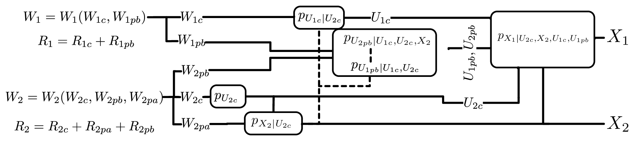
The meaning of the RVs in Theorem V.1 is as follows. Both transmitters perform superposition of two codewords: a common one (to be decoded at both decoders) and a private one (to be decoded at the intended decoder only). In particular:

  • •

    Rate R1R_{1} is split into R1​cR_{1c} and R1​p​bR_{1pb} and conveyed through the RVs U1​cU_{1c} and U1​p​bU_{1pb}, respectively.

  • •

    Rate R2R_{2} is split into R2​cR_{2c}, R2​p​aR_{2pa} and R2​p​bR_{2pb} and conveyed through the RVs U2​c,X2U_{2c},X_{2} and U2​p​bU_{2pb}, respectively.

  • •

    U2​cU_{2c} is the common message of transmitter 2. The subscript “c” stands for “common”.

  • •

    X2X_{2} is the private message of transmitter 2 to be sent by transmitter 2 only. It superimposed to U2​cU_{2c}. The subscript “p” stands for “private” and the subscript “a” stands for “alone”.

  • •

    U1​cU_{1c} is the common message of transmitter 1. It is superimposed to U2​cU_{2c} and - conditioned on U2​cU_{2c} - is binned against X2X_{2}.

  • •

    U1​p​bU_{1pb} and U2​p​bU_{2pb} are private messages of transmitter 1 and transmitter 2, respectively, and are sent by transmitter 1 only. They are binned against one another conditioned on U2​cU_{2c}, as in Marton’s achievable rate region for the broadcast channel [23]. The subscript “b” stands for “broadcast”.

  • •

    X1X_{1} is finally superimposed to all the previous RVs and transmitted over the channel.

A graphical representation of the encoding scheme of Theorem V.1 can be found in Figure 2. The formal description of the proposed encoding scheme is as follows:
Refer to caption
Fig. 2: The achievability encoding scheme of Thm. V.1. The ordering from left to right and the distributions demonstrate the codebook generation process. The dotted lines indicate binning. We see rate splits are used at both users, private messages W1​p​b,W2​p​a,W2​p​bW_{1pb},W_{2pa},W_{2pb} are superimposed on common messages W1​c,W2​cW_{1c},W_{2c} and U1​cU_{1c}, is binned against X2X_{2} conditioned on U2​cU_{2c}, while U1​p​bU_{1pb} and U2​p​bU_{2pb} are binned against each and X2X_{2} other in a Marton-like fashion (conditioned on other subsets of RVs).

V-A Rate splitting

Let W1W_{1} and W2W_{2} be two independent RVs uniformly distributed on [1​…​2N​R1][1...2^{NR_{1}}] and [1​…​2N​R2][1...2^{NR_{2}}] respectively. Consider splitting the messages as follows:

W1=(W1​c,W1​p​b),W2=(W2​c,W2​p​b,W2​p​a),\begin{array}[]{l l l l l l l l l l}W_{1}=(W_{1c},W_{1pb}),\\ W_{2}=(W_{2c},W_{2pb},W_{2pa}),\end{array}

where the messages WiW_{i}, i∈{1​c,2​c,1​p​b,2​p​b,2​p​a}i\in\{1c,2c,1pb,2pb,2pa\}, are all independent and uniformly distributed on [1​…​2N​Ri][1...2^{NR_{i}}], so that the rate are

R1=R1​c+R1​p​b,R2=R2​c+R2​p​a+R2​p​b.\begin{array}[]{l l l l l l l l l l}R_{1}=R_{1c}+R_{1pb},\\ R_{2}=R_{2c}+R_{2pa}+R_{2pb}.\end{array}

V-B Codebook generation

Consider a distribution pU1​c,U2​c,X2,U1​p​b,U1​p​b,X1,X2p_{U_{1c},U_{2c},X_{2},U_{1pb},U_{1pb},X_{1},X_{2}}. The codebooks are generated as follows:

  • •

    Select uniformly at random 2N​R2​c2^{NR_{2c}} length-NN sequences U2​cN​(w2​c)U_{2c}^{N}(w_{2c}), w2​c∈[1​…​2N​R2​c]w_{2c}\in[1...2^{NR_{2c}}], from the typical set TϵN​(pU2​c)T_{\epsilon}^{N}(p_{U_{2c}}).

  • •

    For every w2​c∈[1​…​2N​R2​c]w_{2c}\in[1...2^{NR_{2c}}], select uniformly at random 2N​R2​p​a2^{NR_{2pa}} length-NN sequences X2N​(w2​c,w2​p​a)X_{2}^{N}(w_{2c},w_{2pa}), w2​p​a∈[1​…​2N​R2​p​a]w_{2pa}\in[1...2^{NR_{2pa}}], from the typical set TϵN​(pX2,U2​c|U2​cN​(w2​c))T_{\epsilon}^{N}(p_{X_{2},U_{2c}}|U_{2c}^{N}(w_{2c})).

  • •

    For every w2​c∈[1​…​2N​R2​c]w_{2c}\in[1...2^{NR_{2c}}], select uniformly at random 2N⁡(R1​c+R1​c′)2^{N(R_{1c}+R^{\prime}_{1c})} length-NN sequences U1​cN​(w2​c,w1​c,b0)U_{1c}^{N}(w_{2c},w_{1c},b_{0}), w1​c∈[1​…​2N​R1​c]w_{1c}\in[1...2^{NR_{1c}}] and b0∈[1​…​2N​R1​c′]b_{0}\in[1...2^{NR^{\prime}_{1c}}], from the typical set TϵN​(pU1​c​U2​c|U2​cN​(w2​c))T_{\epsilon}^{N}(p_{U_{1c}U_{2c}}|U_{2c}^{N}(w_{2c}))

  • •

    For every w2​c∈[1​…​2N​R2​c]w_{2c}\in[1...2^{NR_{2c}}], w2​p​a∈[1​…​2N​R2​p​a]w_{2pa}\in[1...2^{NR_{2pa}}], w1​c∈[1​…​2N​R1​c]w_{1c}\in[1...2^{NR_{1c}}] and b0∈[1​…​2N​R1​c′]b_{0}\in[1...2^{NR^{\prime}_{1c}}], select uniformly at random 2N⁡(R2​p​b+R2​p​b′)2^{N(R_{2pb}+R^{\prime}_{2pb})} length-NN sequences U2​p​bN​(w2​c,w2​p​a,w1​c,b0,w2​p​b,b2)U_{2pb}^{N}(w_{2c},w_{2pa},w_{1c},b_{0},w_{2pb},b_{2}), w2​p​b∈[1​…​2N​R2​p​b]w_{2pb}\in[1...2^{NR_{2pb}}] and b2∈[1​…​2N​R2​p​b′]b_{2}\in[1...2^{NR^{\prime}_{2pb}}], from the typical set TϵN​(pU2​p​b,U2​c,U1​c,X2|U2​cN​(w2​c),X2N​(w2​c,w2​p​a),U1​cN​(w2​c,w1​c,b0))T_{\epsilon}^{N}(p_{U_{2pb},U_{2c},U_{1c},X_{2}}|U_{2c}^{N}(w_{2c}),X_{2}^{N}(w_{2c},w_{2pa}),U_{1c}^{N}(w_{2c},w_{1c},b_{0})).

  • •

    For every w2​c∈[1​…​2N​R2​c]w_{2c}\in[1...2^{NR_{2c}}], w1​c∈[1​…​2N​R1​c]w_{1c}\in[1...2^{NR_{1c}}] and b0∈[1​…​2N​R1​c′]b_{0}\in[1...2^{NR^{\prime}_{1c}}], select uniformly at random 2N⁡(R1​p​b+R1​p​b′)2^{N(R_{1pb}+R^{\prime}_{1pb})} length-NN sequences U1​p​bN​(w2​c,w1​c,b0,w1​p​b,b1)U_{1pb}^{N}(w_{2c},w_{1c},b_{0},w_{1pb},b_{1}), w1​p​b∈[1​…​2N​R1​p​b]w_{1pb}\in[1...2^{NR_{1pb}}] and b1∈[1​…​2N​R1​p​b′]b_{1}\in[1...2^{NR^{\prime}_{1pb}}], from the typical set

    TϵN​(pU1​p​b,U2​c,U1​c|U2​cN​(w2​c),U1​cN​(w2​c,w1​c,b0)).\begin{array}[]{l l l l l l l l l l}T_{\epsilon}^{N}(p_{U_{1pb},U_{2c},U_{1c}}|U_{2c}^{N}(w_{2c}),U_{1c}^{N}(w_{2c},w_{1c},b_{0})).\end{array}
  • •

    For every w2​c∈[1​…​2N​R2​c]w_{2c}\in[1...2^{NR_{2c}}], w2​p​a∈[1​…​2N​R2​p​a]w_{2pa}\in[1...2^{NR_{2pa}}], w1​c∈[1​…​2N​R1​c]w_{1c}\in[1...2^{NR_{1c}}], b0∈[1:2N​R1​c′]b_{0}\in[1:2^{NR^{\prime}_{1c}}], w1​p​b∈[1​…​2N​R1​p​b]w_{1pb}\in[1...2^{NR_{1pb}}], b1∈[1:2N​R1​p​b′]b_{1}\in[1:2^{NR^{\prime}_{1pb}}], w2​p​b∈[1​…​2N​R2​p​b]w_{2pb}\in[1...2^{NR_{2pb}}], b2∈[1:2N​R2​p​b′]b_{2}\in[1:2^{NR^{\prime}_{2pb}}], let the channel input X1N​(w2​p​a,w2​c,w1​c,b0,w1​p​b,b1,w2​p​b,b2)X_{1}^{N}(w_{2pa},w_{2c},w_{1c},b_{0},w_{1pb},b_{1},w_{2pb},b_{2}) be any length-NN sequence from the typical set

    TϵN(pX1,U2​c,U1​c,X2,U2​p​b,U1​p​b|U2​cN(w2​c),X2N(w2​c,w2​p​a),U1​cN(w2​c,w1​c,b0),U2​p​bN(w2​c,w2​p​a,w1​c,b0,w2​p​b,b2),OPENU1​p​bN​(w2​c,w1​c,b0,w1​p​b,b1)).\begin{array}[]{l l l l l l l l l l}T_{\epsilon}^{N}(p_{X_{1},U_{2c},U_{1c},X_{2},U_{2pb},U_{1pb}}|U_{2c}^{N}(w_{2c}),X_{2}^{N}(w_{2c},w_{2pa}),U_{1c}^{N}(w_{2c},w_{1c},b_{0}),U_{2pb}^{N}(w_{2c},w_{2pa},w_{1c},b_{0},w_{2pb},b_{2}),\\ U_{1pb}^{N}(w_{2c},w_{1c},b_{0},w_{1pb},b_{1})).\end{array}

V-C Encoding

Given the message w2=(w2​c,w2​p​b,w2​p​a)w_{2}=(w_{2c},w_{2pb},w_{2pa}), encoder 2 sends the codeword X2N​(w2​c,w2​p​a)X_{2}^{N}(w_{2c},w_{2pa}).

Given the message w2=(w2​c,w2​p​b,w2​p​a)w_{2}=(w_{2c},w_{2pb},w_{2pa}) and the message w1=(w1​c,w1​p​b)w_{1}=(w_{1c},w_{1pb}), encoder 1 looks for a triplet (b0,b1,b2)(b_{0},b_{1},b_{2}) such that:

(U2​cN​(w2​c),X2N​(w2​c,w2​p​a),U1​cN​(w2​c,w1​c,b0),U1​p​bN​(w2​c,w1​c,b0,w1​p​b,b1),U2​p​bN​(w2​c,w1​c,b0,w2​p​b,b2))\displaystyle(U_{2c}^{N}(w_{2c}),X_{2}^{N}(w_{2c},w_{2pa}),U_{1c}^{N}(w_{2c},w_{1c},b_{0}),U_{1pb}^{N}(w_{2c},w_{1c},b_{0},w_{1pb},b_{1}),U_{2pb}^{N}(w_{2c},w_{1c},b_{0},w_{2pb},b_{2}))
∈TϵN​(pU2​c,X2,U1​c,U1​p​b,U2​p​b).\displaystyle\in T_{\epsilon}^{N}(p_{U_{2c},X_{2},U_{1c},U_{1pb},U_{2pb}}).

If no such triplet exists, it sets (b0,b1,b2)=(1,1,1)(b_{0},b_{1},b_{2})=(1,1,1). If more than one such triplet exists, it picks one uniformly at random from the found ones. For the selected (b0,b1,b2)(b_{0},b_{1},b_{2}), encoder 1 sends X1N​(w2​p​a,w2​c,w1​c,b0,w1​p​b,b1,w2​p​b,b2)X_{1}^{N}(w_{2pa},w_{2c},w_{1c},b_{0},w_{1pb},b_{1},w_{2pb},b_{2}).

Since the codebooks are generated iid according to

p(codebook)=pU2​c​pX2|U2​c​pU1​c|U2​c​pU2​p​b|U2​c,U1​c,X2​pU1​p​b|U2​c,U1​c\displaystyle p^{\rm(codebook)}=p_{U_{2c}}\,p_{X_{2}|U_{2c}}\,p_{U_{1c}|U_{2c}}\,p_{U_{2pb}|U_{2c},U_{1c},X_{2}}\,p_{U_{1pb}|U_{2c},U_{1c}} (13)

but the encoding forces the actual transmitted codewords to look as if they were generated iid according to

p(encoding)=pU2​c​pX2|U2​c​pU1​c|U2​c,X2​pU2​p​b|U2​c,U1​c,X2​pU1​p​b|U2​c,U1​c,X2,U2​p​b,\displaystyle p^{\rm(encoding)}=p_{U_{2c}}\,p_{X_{2}|U_{2c}}\,p_{U_{1c}|U_{2c},X_{2}}\,p_{U_{2pb}|U_{2c},U_{1c},X_{2}}\,p_{U_{1pb}|U_{2c},U_{1c},X_{2},U_{2pb}}, (14)

We expect the probability of encoding error to depend on

E[p(encoding)p(codebook)]=E[pU1​c|U2​c,X2​pU1​p​b|U2​c,U1​c,X2,U2​p​bpU1​c|U2​c​pU1​p​b|U2​c,U1​c]=I(U1​c;X2|U2​c)+I(U1​p​b;X2,U2​p​b|U2​c,U1​c).E\left[\frac{p^{\rm(encoding)}}{p^{\rm(codebook)}}\right]=E\left[\frac{p_{U_{1c}|U_{2c},X_{2}}\,p_{U_{1pb}|U_{2c},U_{1c},X_{2},U_{2pb}}}{p_{U_{1c}|U_{2c}}\,p_{U_{1pb}|U_{2c},U_{1c}}}\right]=I(U_{1c};X_{2}|U_{2c})+I(U_{1pb};X_{2},U_{2pb}|U_{2c},U_{1c}).

V-D Decoding

Decoder 2 looks for a unique tuple (w2​c,w2​p​a,w2​p​b)(w_{2c},w_{2pa},w_{2pb}) and some (w1​c,b0,b2)(w_{1c},b_{0},b_{2}) such that

(U2​cn​(w2​c),X2n​(w2​c,w2​p​a),U1​cn​(w2​c,w1​c,b0),U2​p​bn​(w2​c,w1​c,b0,w2​p​b,b2),Y2n)∈Tϵn​(pU2​c,X2,U1​c,U2​p​b,Y2).(U_{2c}^{n}(w_{2c}),X_{2}^{n}(w_{2c},w_{2pa}),U_{1c}^{n}(w_{2c},w_{1c},b_{0}),U_{2pb}^{n}(w_{2c},w_{1c},b_{0},w_{2pb},b_{2}),Y_{2}^{n})\in T_{\epsilon}^{n}(p_{U_{2c},X_{2},U_{1c},U_{2pb},Y_{2}}).

Depending on which messages are wrongly decoded at decoder 2, the transmitted sequences and the received Y2nY_{2}^{n} are generated iid according to

p2|⋆≜pU2​c​pX2|U2​c​pU1​c|U2​c​pU2​p​b|U2​c,U1​c,X2​pY2|⋆,\displaystyle p_{2|\star}\triangleq p_{U_{2c}}\,p_{X_{2}|U_{2c}}\,p_{U_{1c}|U_{2c}}\,p_{U_{2pb}|U_{2c},U_{1c},X_{2}}\,p_{Y_{2}|\star}, (15)

where “⋆\star” indicates the messages decoded correctly. However, the actual transmitted sequences and the received Y2nY_{2}^{n} considered at decoder 2 look as if they were generated iid according to

p2≜pU2​c​pX2|U2​c​pU1​c|U2​c,X2​pU2​p​b|U2​c,U1​c,X2​pY2|U2​c,U1​c,X2,U2​p​b.\displaystyle p_{2}\triangleq p_{U_{2c}}\,p_{X_{2}|U_{2c}}\,p_{U_{1c}|U_{2c},X_{2}}\,p_{U_{2pb}|U_{2c},U_{1c},X_{2}}\,p_{Y_{2}|U_{2c},U_{1c},X_{2},U_{2pb}}. (16)

Hence we expect the probability of error at decoder 2 to depend on terms of the type

I2|⋆=E[logp2p2|⋆]=E[logpU1​c|U2​c,X2​pY2|U2​c,U1​c,X2,U2​p​bpU1​c|U2​c​pY2|⋆]=I(U1​c;X2|U2​c)+I(Y2;U2​c,U1​c,X2,U2​p​b|⋆).\displaystyle I_{2|\star}=E\left[\log\frac{p_{2}}{p_{2|\star}}\right]=E\left[\log\frac{p_{U_{1c}|U_{2c},X_{2}}\,p_{Y_{2}|U_{2c},U_{1c},X_{2},U_{2pb}}}{p_{U_{1c}|U_{2c}}\,p_{Y_{2}|\star}}\right]=I(U_{1c};X_{2}|U_{2c})+I(Y_{2};U_{2c},U_{1c},X_{2},U_{2pb}|\star). (17)

Decoder 1 looks for a unique pair (w1​c,w1​p​b)(w_{1c},w_{1pb}) and some (w2​c,b0,b1)(w_{2c},b_{0},b_{1}) such that

(U2​cn​(w2​c),U1​cn​(w2​c,w1​c,b0),U1​p​bn​(w2​c,w1​c,b0,w1​p​b,b1),Y1n)∈Tϵn​(pU2​c,U1​c,U1​p​b,Y1).(U_{2c}^{n}(w_{2c}),U_{1c}^{n}(w_{2c},w_{1c},b_{0}),U_{1pb}^{n}(w_{2c},w_{1c},b_{0},w_{1pb},b_{1}),Y_{1}^{n})\in T_{\epsilon}^{n}(p_{U_{2c},U_{1c},U_{1pb},Y_{1}}).

Depending on which messages are wrongly decoded at decoder 1, the transmitted sequences and the received Y1nY_{1}^{n} are generated iid according to

p1|⋆≜pU2​c​pU1​c|U2​c​pU1​p​b|U2​c,U1​c​pY1|⋆,\displaystyle p_{1|\star}\triangleq p_{U_{2c}}\,p_{U_{1c}|U_{2c}}\,p_{U_{1pb}|U_{2c},U_{1c}}\,p_{Y_{1}|\star}, (18)

where “⋆\star” indicates the messages decoded correctly. However, the actual transmitted sequences and the received Y1nY_{1}^{n} considered at decoder 1 look as if they were generated iid according to

p1≜pU2​c​pU1​c|U2​c​pU1​p​b|U2​c,U1​c​pY1|U2​c,U1​c,U1​p​b.\displaystyle p_{1}\triangleq p_{U_{2c}}\,p_{U_{1c}|U_{2c}}\,p_{U_{1pb}|U_{2c},U_{1c}}\,p_{Y_{1}|U_{2c},U_{1c},U_{1pb}}. (19)

Hence we expect the probability of error at decoder 1 to depend on terms of the type

I1|⋆=E[logp1p1|⋆]=E[logpY1|U2​c,U1​c,U1​p​bpY1|⋆]=I(Y1;U2​c,U1​c,U1​p​b|⋆).\displaystyle I_{1|\star}=E\left[\log\frac{p_{1}}{p_{1|\star}}\right]=E\left[\log\frac{p_{Y_{1}|U_{2c},U_{1c},U_{1pb}}}{p_{Y_{1}|\star}}\right]=I(Y_{1};U_{2c},U_{1c},U_{1pb}|\star). (20)

The error analysis is found in Appendix -A. ∎

V-E Two step binning

It is also possible to perform binning in a sequential manner. First, U1​cU_{1c} is binned against X1X_{1}, and then U1​p​bU_{1pb} and U2​p​bU_{2pb} are binned against each other conditioned on (U2​c,U1​c)(U_{2c},U_{1c}) and (U2​c,X2,U1​c)(U_{2c},X_{2},U_{1c}) respectively. With respect to the encoding operation of the previous section, this affects Section V-C as follows:

Given the message w2=(w2​c,w2​p​b,w2​p​a)w_{2}=(w_{2c},w_{2pb},w_{2pa}) and the message w1=(w1​c,w1​p​b)w_{1}=(w_{1c},w_{1pb}), encoder 1 looks for b0b_{0} such that

(U2​cN​(w2​c),X2N​(w2​c,w2​p​a),U1​cN​(w2​c,w1​c,b0)CLOSE,\displaystyle(U_{2c}^{N}(w_{2c}),X_{2}^{N}(w_{2c},w_{2pa}),U_{1c}^{N}(w_{2c},w_{1c},b_{0}),
∈TϵN​(pU2​c,X2,U1​c).\displaystyle\in T_{\epsilon}^{N}(p_{U_{2c},X_{2},U_{1c}}).

If no such b0b_{0} exists, it sets b0=1b_{0}=1. If more than one such b0b_{0} exists, it picks one uniformly at random. For the selected b0b_{0}, encoder 1 looks for (b1,b2)(b_{1},b_{2}) such that:

(U2​cN​(w2​c),X2N​(w2​c,w2​p​a),U1​cN​(w2​c,w1​c,b0),U1​p​bN​(w2​c,w1​c,b0,w1​p​b,b1),U2​p​bN​(w2​c,w1​c,b0,w2​p​b,b2))\displaystyle(U_{2c}^{N}(w_{2c}),X_{2}^{N}(w_{2c},w_{2pa}),U_{1c}^{N}(w_{2c},w_{1c},b_{0}),U_{1pb}^{N}(w_{2c},w_{1c},b_{0},w_{1pb},b_{1}),U_{2pb}^{N}(w_{2c},w_{1c},b_{0},w_{2pb},b_{2}))
∈TϵN​(pU2​c,X2,U1​c,U1​p​b,U2​p​b).\displaystyle\in T_{\epsilon}^{N}(p_{U_{2c},X_{2},U_{1c},U_{1pb},U_{2pb}}).

If no such (b1,b2)(b_{1},b_{2}) exists, it sets (b1,b2)=(1,1)(b_{1},b_{2})=(1,1). If more than one such (b1,b2)(b_{1},b_{2}) exists, it picks one uniformly at random from the found ones.

For the selected (b0,b1,b2)(b_{0},b_{1},b_{2}), encoder 1 sends X1N​(w2​p​a,w2​c,w1​c,b0,w1​p​b,b1,w2​p​b,b2)X_{1}^{N}(w_{2pa},w_{2c},w_{1c},b_{0},w_{1pb},b_{1},w_{2pb},b_{2}).

The next lemma states the condition under which this two step encoding procedure is successful with high probability.

Lemma V.3.

The two-step binning encoding procedure of Section V-E is successful if

R1​c′\displaystyle R^{\prime}_{1c} ≥\displaystyle\geq I⁡(U1​c;X2|U2​c),\displaystyle I(U_{1c};X_{2}|U_{2c}), (21a)
R1​p​b′\displaystyle R^{\prime}_{1pb} ≥\displaystyle\geq I(U1​p​b;X2|U2​c,U1​c),\displaystyle I(U_{1pb};X_{2}|U_{2c},U_{1c}), (21b)
R1​p​b′+R2​p​b′\displaystyle R^{\prime}_{1pb}+R^{\prime}_{2pb} ≥\displaystyle\geq I(U1​p​b;X2,U2​p​b|U2​c,U1​c).\displaystyle I(U_{1pb};X_{2},U_{2pb}|U_{2c},U_{1c}). (21c)

The proof of the lemma is found in Appendix (-E).

Remark V.4.

Since the binning rate (12a) of Theorem V.1 can be taken with equality, the two step binning has the same performance as joint binning. In fact, by setting (21a)(\ref{eq: two step binning R"1c}) to hold with equality, we obtain the equality between the binning rate expression of the joint binning and the two step binning.

A plot of the permissible binning rates R1​p​bR_{1pb} and R2​p​bR_{2pb} is depicted in Figure 3.

Refer to caption
Fig. 3: The region of the admissible binning rates R1​p​bR_{1pb} and R2​p​bR_{2pb} in Theorem V.1.

VI Comparison with existing achievable rate regions

We now show that the region of Theorem V.1 contains all other known achievable rate regions for the DM-CIFC. Showing inclusion of the rate regions [26, Thm.2], [24, Thm. 1] and [25, Thm. 4.1] is sufficient to demonstrate the largest known DM-CIFC region, since the region of [26, Thm.2] (first presented in [10]) is shown (in [26]) to contain those of [8, Thm. 1] and [20].

VI-A Devroye et al.’s region [24, Thm. 1]

In Appendix -F we show that the region of [24, Thm. 1] ℛD​M​T{\cal R}_{DMT}, is contained in our new region ℛR​T​D{\cal R}_{RTD} along the lines:

∙\bullet We make a correspondence between the random variables and corresponding rates of ℛD​M​T{\cal R}_{DMT} and ℛR​T​D{\cal R}_{RTD}.
∙\bullet We define new regions ℛD​M​T⊆ℛD​M​To​u​t\mathcal{R}_{DMT}\subseteq\mathcal{R}_{DMT}^{out} and ℛR​T​Di​n⊆ℛR​T​D\mathcal{R}_{RTD}^{in}\subseteq\mathcal{R}_{RTD} which are easier to compare: they have identical input distribution decompositions and similar rate equations.
∙\bullet For any fixed input distribution, an equation-by-equation comparison leads to ℛD​M​T⊆ℛD​M​To​u​t⊆ℛR​T​Di​n⊆ℛR​T​D\mathcal{R}_{DMT}\subseteq\mathcal{R}_{DMT}^{out}\subseteq\mathcal{R}_{RTD}^{in}\subseteq\mathcal{R}_{RTD}.

VI-B Cao and Chen’s region [26, Thm. 2]

The region in [26, Thm. 2] uses a similar encoding structure as that of ℛR​T​D\mathcal{R}_{RTD} with two exceptions:

1) The binning is done sequentially rather than jointly as in ℛR​T​D\mathcal{R}_{RTD} leading to binning constraints (43)–(45) in [26, Thm. 2] as opposed to (12a)–(12c) in Thm.V.1. Notable is that both schemes have adopted a Marton-like binning scheme at the cognitive transmitter, as first introduced in the context of the CIFC in [10].

2) While the cognitive messages are rate-split in identical fashions, the primary message is split into 2 parts in [26, Thm. 2] (R1=R11+R10R_{1}=R_{11}+R_{10}, note the reversal of indices) while we explicitly split the primary message into three parts R2=R2​c+R2​p​a+R2​p​bR_{2}=R_{2c}+R_{2pa}+R_{2pb}. In Appendix -G we show that the region of [26, Thm.2], denoted as ℛC​C⊆ℛR​T​D{\cal R}_{CC}\subseteq{\cal R}_{RTD} in two steps:

∙\bullet We first show that we may WLOG set U11=∅U_{11}=\emptyset in [26, Thm.2], creating a new region RC​C′R_{CC}^{\prime}.

∙\bullet We next make a correspondence between our RVs and those of [26, Thm.2] and obtain identical regions.

VI-C Jiang et al.’s region [25, Thm. 4.1]

The scheme originally designed for the more general broadcast channel with cognitive relays (or interference-chanel with a cognitive relay) may be tailored/reduced to derive a region for the cognitive interference channel. This scheme also incorporates a broadcasting strategy. However, the common messages are created independently instead of having the common message from transmitter 1 superposed to the common message from transmitter 2. The former choice introduces more rate constraints than the latter and allows us to show inclusion in ℛR​T​D\mathcal{R}_{RTD} after equating random variables. The proof of the containment of the achievable region of [25, Thm. 4.1] in ℛR​T​D\mathcal{R}_{RTD} is found in Appendix -H.

VII New capacity results for the DM-CIFC

We now look at the expression of the outer bound [4, Thm. 3.1] to gain insight into potentially capacity achieving achievable schemes. In particular we look at the expression of the corner points of the outer bound region for a fixed pU,X1,X2p_{U,X_{1},X_{2}} and try to interpret the RVs as private and common messages to be decoded at the transmitter side. We then consider an achievable scheme inspired by these observations and show that schemes achieve capacity for a particular class of channels. This class of channels contains the “very strong” and the “very weak” interference regimes and thus corresponds to the largest class of channels for which capacity is currently known.

The outer bound region of [4, Thm. 3.1] has at most two corner points where both R1R_{1} and R2R_{2} are non zero:

(R1o​u​t​(a),R2o​u​t​(a))=(I(Y1;X1|U,X2),I(Y2;U,X2))\displaystyle(R_{1}^{out\ (a)},R_{2}^{out\ (a)})=\left(I(Y_{1};X_{1}|U,X_{2}),I(Y_{2};U,X_{2})\right) (22)
(R1o​u​t​(b),R2o​u​t​(b))=(I(Y1;X1|U,X2)+I(Y2;U,X2)−Δ,Δ)\displaystyle(R_{1}^{out\ (b)},R_{2}^{out\ (b)})=\left(I(Y_{1};X_{1}|U,X_{2})+I(Y_{2};U,X_{2})-\Delta,\Delta\right) (23)
Δ=[I⁡(Y2,U,X2)−I⁡(Y1;U|X2)]+,\displaystyle\ \ \ \ \ \Delta=[I(Y_{2};U,X_{2})-I(Y_{1};U|X_{2})]^{+},

since

R2o​u​t​(a)=min{I(Y2;U,X2),I(Y2;U,X2)+I(Y1;X1|U,X2)}=I(Y2;U,X2),R1o​u​t​(a)=min{I(Y1;X1|U,X2),I(Y1;X1|X2)}=I(Y1;X1|U,X2),\begin{array}[]{l l l l l l l l l l}R_{2}^{out\ (a)}&=\min\{I(Y_{2};U,X_{2}),I(Y_{2};U,X_{2})+I(Y_{1};X_{1}|U,X_{2})\}=I(Y_{2};U,X_{2}),\\ R_{1}^{out\ (a)}&=\min\{I(Y_{1};X_{1}|U,X_{2}),I(Y_{1};X_{1}|X_{2})\}=I(Y_{1};X_{1}|U,X_{2}),\end{array}

and

R2o​u​t​(b)=min{I(Y2;U,X2),I(Y2;U,X2)+I(Y1;X1|U,X2)−I(Y1;X1|X2)}=[I(Y2;U,X2)+min{0,I(Y1;X1|U,X2)−I(Y1;X1,U|X2)}]+=[I⁡(Y2,U,X2)−I⁡(Y1;U|X2)]+≜Δ,R1o​u​t​(b)≤min{I(Y1;X1|X2),I(Y2;U,X2)+I(Y1;X1|U,X2)}=I(Y1;X1|U,X2)+I(Y2;U,X2)−max{I(Y2;U,X2)−I(Y1;U|X2),0}=I(Y1;X1|U,X2)+I(Y2;U,X2)−Δ.\begin{array}[]{l l l l l l l l l l}R_{2}^{out\ (b)}&=\min\{I(Y_{2};U,X_{2}),I(Y_{2};U,X_{2})+I(Y_{1};X_{1}|U,X_{2})-I(Y_{1};X_{1}|X_{2})\}\\ &=[I(Y_{2};U,X_{2})+\min\{0,I(Y_{1};X_{1}|U,X_{2})-I(Y_{1};X_{1},U|X_{2})\}]^{+}\\ &=[I(Y_{2};U,X_{2})-I(Y_{1};U|X_{2})]^{+}\triangleq\Delta,\\ R_{1}^{out\ (b)}&\leq\min\{I(Y_{1};X_{1}|X_{2}),I(Y_{2};U,X_{2})+I(Y_{1};X_{1}|U,X_{2})\}\\ &=I(Y_{1};X_{1}|U,X_{2})+I(Y_{2};U,X_{2})-\max\{I(Y_{2};U,X_{2})-I(Y_{1};U|X_{2}),0\}\\ &=I(Y_{1};X_{1}|U,X_{2})+I(Y_{2};U,X_{2})-\Delta.\\ \end{array}

Proving the achievability of both these corner points for any pU,X1,X2p_{U,X_{1},X_{2}} shows capacity by a simple time sharing argument.

We can now look at the corner point expression and try to draw some intuition on the achievable schemes that can possibly achieve these rates. For the corner point (R1(a),R2(a))(R_{1}^{(a)},R_{2}^{(a)}) we can interpret (U,X2)(U,X_{2}) as a common message from transmitter 2 to receiver 2 that is also decoded at receiver 1. X1X_{1} is superposed to (U,X2)(U,X_{2}) since the decoding of X1X_{1} follows the one of (U,X2)(U,X_{2}) at decoder 2.

The corner point (R1o​u​t​(b),R2o​u​t​(b))(R_{1}^{out\ (b)},R_{2}^{out\ (b)}) has two possible expressions:

1) If I⁡(Y1;U|X2)≤I⁡(Y2,U,X2)I(Y_{1};U|X_{2})\leq I(Y_{2};U,X_{2}) we have that

(R1o​u​t​(b)′,R2o​u​t​(b)′)=(I⁡(Y1;X1,U|X2),I⁡(Y2,U,X2)−I⁡(Y1;U|X2)),\displaystyle(R_{1}^{out\ (b)^{\prime}},R_{2}^{out\ (b)^{\prime}})=\left(I(Y_{1};X_{1},U|X_{2}),I(Y_{2};U,X_{2})-I(Y_{1};U|X_{2})\right), (24)

which suggests that X2X_{2} is again the common primary message and the cognitive message is divided into a public and private part, UU and X1X_{1} respectively.

2) If I⁡(Y1;U|X2)>I⁡(Y2,U,X2)I(Y_{1};U|X_{2})>I(Y_{2};U,X_{2}) we have that

(R1o​u​t​(b)​",R2o​u​t​(b)​")=(I⁡(Y2,U,X2)+I⁡(Y1;X1,U|X2),0).\displaystyle(R_{1}^{out\ (b)"},R_{2}^{out\ (b)"})=\left(I(Y_{2};U,X_{2})+I(Y_{1};X_{1},U|X_{2}),0\right). (25)

In this case the outer bound has only one corner point where both rates are non zero. Note that we can always achieve the point

(R1i​n​(b)​",R2i​n​(b)​")=(I⁡(Y1;X1,U|X2),0)(R_{1}^{in\ (b)"},R_{2}^{in\ (b)"})=\left(I(Y_{1};X_{1},U|X_{2}),0\right)

by having transmitter 2 send a known signal. In this case we have R2o​u​t​(b)​"=R2i​n​(b)​"R_{2}^{out\ (b)"}=R_{2}^{in\ (b)"} and R1o​u​t​(b)​"≤R1i​n​(b)​"R_{1}^{out\ (b)"}\leq R_{1}^{in\ (b)"} since

I⁡(Y1;X1,U|X2)≥I⁡(Y2,U,X2)+I⁡(Y1;X1,U|X2)I⁡(Y1;U|X2)>I⁡(Y2,U,X2).\begin{array}[]{l l l l l l l l l l}I(Y_{1};X_{1},U|X_{2})\geq I(Y_{2};U,X_{2})+I(Y_{1};X_{1},U|X_{2})\\ I(Y_{1};U|X_{2})>I(Y_{2};U,X_{2}).\end{array}

So in this case showing the achievability of the point in equation (23) is sufficient to show capacity.

Guided by these observations, we consider a scheme that has only the components U2​c,U1​cU_{2c},U_{1c} and U1​p​bU_{1pb}. That is, the primary message ω2\omega_{2} is common and the cognitive message ω1\omega_{1} is split into a private and a public message. With this scheme we are able to extend the capacity results in the “very weak interference” of Theorem III.5 and the “very strong interference” of Theorem III.6. This scheme coincides with the scheme of [27] which achieves capacity if the cognitive receiver is required to decode both messages (with and without the secrecy constraint).

Theorem VII.1.

Capacity in the “better cognitive decoding” regime.

When the following condition holds

I⁡(Y1,X2,U)≥I⁡(Y2,X2,U)∀pX1,X2,U,\displaystyle I(Y_{1};X_{2},U)\geq I(Y_{2};X_{2},U)\ \ \ \ \ \forall p_{X_{1},X_{2},U}, (26)

the capacity region of the DM-CIFC is given by region in (1).

Proof.

Consider the achievable rate region of Theorem V.1 when setting

X1=U1​p​bX2=U2​c=U2​p​b\begin{array}[]{l l l l l l l l l l}X_{1}=U_{1pb}\\ X_{2}=U_{2c}=U_{2pb}\\ \end{array}

so that

R2=R2​cR2​p​a=R2​p​b=0R1​c′=R1​p​b′=R2​p​b′=0.\begin{array}[]{l l l l l l l l l l}R_{2}=R_{2c}\\ R_{2pa}=R_{2pb}=0\\ R_{1c}^{\prime}=R_{1pb}^{\prime}=R_{2pb}^{\prime}=0.\end{array}

In the resulting scheme, the message from transmitter 2 to receiver 2 is all common while the message from transmitter 1 to receiver 1 is split into common and private parts. The achievable region of this sub-scheme is:

R2+R1​c\displaystyle R_{2}+R_{1c} ≤\displaystyle\leq I⁡(Y2,U1​c,X2)\displaystyle I(Y_{2};U_{1c},X_{2}) (27a)
R2+R1​c+R1​p​b\displaystyle R_{2}+R_{1c}+R_{1pb} ≤\displaystyle\leq I⁡(Y1,U1​c,X2)\displaystyle I(Y_{1};U_{1c},X_{2}) (27b)
R1​c+R1​p​b\displaystyle R_{1c}+R_{1pb} ≤\displaystyle\leq I⁡(Y1;U1​c,X1|U2​c)\displaystyle I(Y_{1};U_{1c},X_{1}|U_{2c}) (27c)
R1​p​b\displaystyle R_{1pb} ≤\displaystyle\leq I(Y1;X1|X2,U1​c).\displaystyle I(Y_{1};X_{1}|X_{2},U_{1c}). (27d)

By applying Fourier-Motzkin elimination [28] we obtain the achievable rate region

R1\displaystyle R_{1} ≤\displaystyle\leq I⁡(Y1;U1​c,X1|X2)\displaystyle I(Y_{1};U_{1c},X_{1}|X_{2}) (28a)
R2\displaystyle R_{2} ≤\displaystyle\leq I⁡(Y2,U1​c,X2)\displaystyle I(Y_{2};U_{1c},X_{2}) (28b)
R1+R2\displaystyle R_{1}+R_{2} ≤\displaystyle\leq I(Y2;U1​c,X2)+I(Y1;X1|X2,U1​c)\displaystyle I(Y_{2};U_{1c},X_{2})+I(Y_{1};X_{1}|X_{2},U_{1c}) (28c)
R1+R2\displaystyle R_{1}+R_{2} ≤\displaystyle\leq I⁡(Y1,X2,U1​c,X1).\displaystyle I(Y_{1};X_{2},U_{1c},X_{1}). (28d)
B

y letting U1​c=UU_{1c}=U we see that (1a) matches (28a), (1b) matches (28b), (1c) matches (28c), and (28d) is redundant when

I(Y1;X2,X1,U)≥I(Y2;U,X2)+I(Y1;X1|X2,U),I(Y_{1};X_{2},X_{1},U)\geq I(Y_{2};U,X_{2})+I(Y_{1};X_{1}|X_{2},U),

or equivalently when

I⁡(Y1,U,X2)≥I⁡(Y2,U,X2).\displaystyle I(Y_{1};U,X_{2})\geq I(Y_{2};U,X_{2}). (29)

∎

We term the condition in equation (29) “better cognitive decoding” since decoder 1 has a higher mutual information between its received channel output and the RVs UU and X2X_{2} than the primary receiver.

Remark VII.2.

The “better cognitive decoding” in (29) is looser than both the “very weak interference” condition of (7) and the “very strong interference” condition of (8). In fact summing the two equations of condition (7) we have

I⁡(U;Y1|X2)+I⁡(X2,Y1)≥I⁡(U;Y2|X2)+I⁡(X2,Y2)⟺I⁡(Y1,U,X2)≥I⁡(Y2,U,X2)\begin{array}[]{l l l l l l l l l l}I(U;Y_{1}|X_{2})+I(X_{2};Y_{1})\geq I(U;Y_{2}|X_{2})+I(X_{2};Y_{2})\Longleftrightarrow I(Y_{1};U,X_{2})\geq I(Y_{2};U,X_{2})\end{array}

which corresponds to condition (29). Similarly by summing the two equation of condition (8) we obtain

I⁡(Y1,X1,X2)+I⁡(X1;Y2|X2)≥I⁡(Y2,X1,X2)+I⁡(X1;Y1|X2)⟺I⁡(Y1,X1,X2)−I⁡(X1;Y1|X2)≥I⁡(Y2,X1,X2)−I⁡(X1;Y2|X2)⟺I⁡(Y1,X1,X2,U)−I⁡(X1;Y1|X2)≥I⁡(Y2,X1,X2,U)−I⁡(X1;Y2|X2)⟺I⁡(Y1,X2,U)≥I⁡(Y2,X2,U)\begin{array}[]{l l l l l l l l l l}I(Y_{1};X_{1},X_{2})+I(X_{1};Y_{2}|X_{2})&\geq&I(Y_{2};X_{1},X_{2})+I(X_{1};Y_{1}|X_{2})\Longleftrightarrow\\ I(Y_{1};X_{1},X_{2})-I(X_{1};Y_{1}|X_{2})&\geq&I(Y_{2};X_{1},X_{2})-I(X_{1};Y_{2}|X_{2})\Longleftrightarrow\\ I(Y_{1};X_{1},X_{2},U)-I(X_{1};Y_{1}|X_{2})&\geq&I(Y_{2};X_{1},X_{2},U)-I(X_{1};Y_{2}|X_{2})\Longleftrightarrow\\ I(Y_{1};X_{2},U)&\geq&I(Y_{2};X_{2},U)\\ \end{array}

which again corresponds to condition (29).

Since both (7) and (8) imply the (29), we conclude that (29) is more general than the previous two.

The scheme that achieves capacity in very weak interference is obtained by setting U1​c=X2U_{1c}=X_{2} so that all the cognitive message is private and the primary message is common. The scheme that achieves capacity in very strong interference is obtained by setting U1​c=X1U_{1c}=X_{1} so that both transmitters send only public messages. The scheme that we use to show the achievability in the “strong cognitive decoding” regime mixes these two schemes by splitting the cognitive message into public and private messages. This relaxes the strong interference achievability conditions as now the cognitive encoder needs to decode only part of the cognitive message. The scheme also relaxes the very weak achievability condition since it allows the cognitive encoder to decode part of the cognitive message and remove its unwanted effects. For this reason, the resulting achievability conditions are looser than both cases.

VIII Capacity for the semi-deterministic CIFC

Consider the specific class of DM-CIFC for which the signal received at receiver 1 is a deterministic function of the channel inputs, that is

Y1=f1​(X1,X2).\displaystyle Y_{1}=f_{1}(X_{1},X_{2}). (30)

This class of channels is termed semi-deterministic CIFC and it was first introduced in [26]. In [26] the capacity region is derived for the case I⁡(Y1,X2)≥I⁡(Y2,X2)I(Y_{1};X_{2})\geq I(Y_{2};X_{2}); we extend this result by determining the capacity region in general (no extra conditions). Note that the authors of [26] consider the case where f1f_{1} is invertible; we do not require this condition.

Theorem VIII.1.

The capacity region of the semi-deterministic cognitive interference channel such that (30) consists of all (R1,R2)∈ℝ+2(R_{1},R_{2})\in{\mathbb{R}}_{+}^{2} such that

R1\displaystyle R_{1} ≤\displaystyle\leq H⁡(Y1|X2)\displaystyle H(Y_{1}|X_{2}) (31a)
R2\displaystyle R_{2} ≤\displaystyle\leq I⁡(Y2,U,X2)\displaystyle I(Y_{2};U,X_{2}) (31b)
R1+R2\displaystyle R_{1}+R_{2} ≤\displaystyle\leq I⁡(Y2,U,X2)+H⁡(Y1|U,X2)\displaystyle I(Y_{2};U,X_{2})+H(Y_{1}|U,X_{2}) (31c)

taken over the union of all distributions pU,X1,X2p_{U,X_{1},X_{2}}.

Proof.

Outer bound: The outer bound is obtained from Theorem III.1 “one auxiliary RV outer bound” , by using the deterministic condition in (30).

Achievability: Consider the scheme with only the RVs X2X_{2}, U1​p​bU_{1pb} and U2​p​bU_{2pb}, obtained by setting U2​c=U1​c=∅U_{2c}=U_{1c}=\emptyset. The achievable rate region of Theorem V.1 becomes:

R1​p​b′\displaystyle R^{\prime}_{1pb} ≥\displaystyle\geq I⁡(U1​p​b,X2)\displaystyle I(U_{1pb};X_{2}) (32a)
R1​p​b′+R2​p​b′\displaystyle R^{\prime}_{1pb}+R^{\prime}_{2pb} ≥\displaystyle\geq I⁡(U1​p​b,U2​p​b,X2)\displaystyle I(U_{1pb};U_{2pb},X_{2}) (32b)
R2​p​a+R2​p​b+R2​p​b′\displaystyle R_{2pa}+R_{2pb}+R^{\prime}_{2pb} ≤\displaystyle\leq I⁡(Y2,U2​p​b,X2)\displaystyle I(Y_{2};U_{2pb},X_{2}) (32c)
R2​p​b+R2​p​b′\displaystyle R_{2pb}+R^{\prime}_{2pb} ≤\displaystyle\leq I⁡(Y2;U2​p​b|X2)\displaystyle I(Y_{2};U_{2pb}|X_{2}) (32d)
R1​p​b+R1​p​b′\displaystyle R_{1pb}+R^{\prime}_{1pb} ≤\displaystyle\leq I⁡(Y1,U1​p​b),\displaystyle I(Y_{1};U_{1pb}), (32e)

taken over the union of all input distributions pU1​p​b,U2​p​b,X1,X2​pY1,Y2|X1,X2p_{U_{1pb},U_{2pb},X_{1},X_{2}}p_{Y_{1},Y_{2}|X_{1},X_{2}}.

From the Fourier Motzkin elimination of this sub-scheme, we see that we can set R2​p​b=0R_{2pb}=0 without loss of generality and that the region can be rewritten as

ℛ0(U1​p​b,U2​p​b,X2)=Δ{\displaystyle{\cal R}_{0}(U_{1pb},U_{2pb},X_{2})\stackrel{{\scriptstyle\Delta}}{{=}}\{ R1\displaystyle R_{1} ≤I⁡(Y1,U1​p​b)−I⁡(U1​p​b,X2)\displaystyle\leq I(Y_{1};U_{1pb})-I(U_{1pb};X_{2}) (33a)
R1\displaystyle R_{1} ≤I⁡(Y2;U2​p​b|X2)−I⁡(U1​p​b;U2​p​b|X2)+I⁡(Y1,U1​p​b)−I⁡(U1​p​b,X2)\displaystyle\leq I(Y_{2};U_{2pb}|X_{2})-I(U_{1pb};U_{2pb}|X_{2})+I(Y_{1};U_{1pb})-I(U_{1pb};X_{2}) (33b)
R2\displaystyle R_{2} ≤I⁡(Y2,U2​p​b,X2)\displaystyle\leq I(Y_{2};U_{2pb},X_{2}) (33c)
R1+R2\displaystyle R_{1}+R_{2} ≤I(Y2;U2​p​b,X2)+I(Y1;U1​p​b)−I(U1​p​b;U2​p​b,X2)}\displaystyle\leq I(Y_{2};U_{2pb},X_{2})+I(Y_{1};U_{1pb})-I(U_{1pb};U_{2pb},X_{2})\} (33d)

taken over the union of all distributions that factor as

pU1​p​b,U2​p​b,X1,X2​pY1,Y2|X1,X2.\displaystyle p_{U_{1pb},U_{2pb},X_{1},X_{2}}p_{Y_{1},Y_{2}|X_{1},X_{2}}. (34)

Let

ℛ1(U1​p​b,U2​p​b,X2)=Δ{\displaystyle{\cal R}_{1}(U_{1pb},U_{2pb},X_{2})\stackrel{{\scriptstyle\Delta}}{{=}}\{ R1\displaystyle R_{1} ≤I⁡(Y1,U1​p​b)−I⁡(U1​p​b,X2)\displaystyle\leq I(Y_{1};U_{1pb})-I(U_{1pb};X_{2}) (35a)
R2\displaystyle R_{2} ≤I⁡(Y2,U2​p​b,X2)\displaystyle\leq I(Y_{2};U_{2pb},X_{2}) (35b)
R1+R2\displaystyle R_{1}+R_{2} ≤I(Y2;U2​p​b,X2)+I(Y1;U1​p​b)−I(U1​p​b;U2​p​b,X2)}\displaystyle\leq I(Y_{2};U_{2pb},X_{2})+I(Y_{1};U_{1pb})-I(U_{1pb};U_{2pb},X_{2})\} (35c)

and

ℛ2(U1​p​b,X2)=Δ{\displaystyle{\cal R}_{2}(U_{1pb},X_{2})\stackrel{{\scriptstyle\Delta}}{{=}}\{ R1\displaystyle R_{1} ≤I⁡(Y1,U1​p​b)−I⁡(U1​p​b,X2)\displaystyle\leq I(Y_{1};U_{1pb})-I(U_{1pb};X_{2}) (36a)
R2\displaystyle R_{2} ≤I(Y2;X2)}.\displaystyle\leq I(Y_{2};X_{2})\}. (36b)

Notice that

ℛ2​(U1​p​b,X2)⊆ℛ1​(U1​p​b,U2​p​b,X2)⊆ℛ0​(U1​p​b,U2​p​b,X2),{\cal R}_{2}(U_{1pb},X_{2})\subseteq{\cal R}_{1}(U_{1pb},U_{2pb},X_{2})\subseteq{\cal R}_{0}(U_{1pb},U_{2pb},X_{2}),

since

ℛ2​(U1​p​b,X2)=ℛ1​(U1​p​b,U2​p​b=X2,X2)=ℛ0​(U1​p​b,U2​p​b=X2,X2),{\cal R}_{2}(U_{1pb},X_{2})={\cal R}_{1}(U_{1pb},U_{2pb}=X_{2},X_{2})={\cal R}_{0}(U_{1pb},U_{2pb}=X_{2},X_{2}),

and ℛ0​(U1​p​b,U2​p​b,X2){\cal R}_{0}(U_{1pb},U_{2pb},X_{2}) has one less constraint than ℛ1​(U1​p​b,U2​p​b,X2){\cal R}_{1}(U_{1pb},U_{2pb},X_{2}).

We now wish to show that

⋃pX2,U1​p​b,U2​p​bℛ0=⋃pX2,U1​p​b,U2​p​bℛ1,\begin{array}[]{l l l l l l l l l l}\bigcup_{p_{X_{2},U_{1pb},U_{2pb}}}{\cal R}_{0}=\bigcup_{p_{X_{2},U_{1pb},U_{2pb}}}{\cal R}_{1},\end{array}

that is, equation (33b) can be removed from the Fourier Motzkin eliminated region of (32). The proof of this equivalence follows that of [29, Lemma 2]. For P⁡(U1​p​b,U2​p​b,X2)P(U_{1pb},U_{2pb},X_{2}) such that

I⁡(Y2;U2​p​b|X2)−I⁡(U1​p​b;U2​p​b|X2)≥0I(Y_{2};U_{2pb}|X_{2})-I(U_{1pb};U_{2pb}|X_{2})\geq 0

we have

ℛ1​(U1​p​b,U2​p​b,X2)=ℛ0​(U1​p​b,U2​p​b,X2).{\cal R}_{1}(U_{1pb},U_{2pb},X_{2})={\cal R}_{0}(U_{1pb},U_{2pb},X_{2}).

For those P⁡(U1​p​b,U2​p​b,X2)P(U_{1pb},U_{2pb},X_{2}) such that

I⁡(Y2;U2​p​b|X2)−I⁡(U1​p​b;U2​p​b|X2)<0I(Y_{2};U_{2pb}|X_{2})-I(U_{1pb};U_{2pb}|X_{2})<0

we have that the point

OPEN(R1,R2)=(I⁡(Y1,U1​p​b)−I⁡(U1​p​b,X2)),I⁡(Y2,X2))(R_{1},R_{2})=(I(Y_{1};U_{1pb})-I(U_{1pb};X_{2})),I(Y_{2};X_{2}))

is achievable in ℛ2\mathcal{R}_{2}. This point lies inside ℛ1{\cal R}_{1} and ℛ0{\cal R}_{0} and satisfies all the rate constraints in (33) but (33b). In particular, the sum rate equation (33d) given by

R1+R2≤I⁡(Y2,U2​p​b,X2)+I⁡(Y1,U1​p​b)−I⁡(U1​p​b,U2​p​b,X2),R_{1}+R_{2}\leq I(Y_{2};U_{2pb},X_{2})+I(Y_{1};U_{1pb})-I(U_{1pb};U_{2pb},X_{2}),

which implies

R2≤I⁡(Y2,X2)R_{2}\leq I(Y_{2};X_{2})

since

R2≤I⁡(Y2,U2​p​b,X2)+I⁡(Y1,U1​p​b)−I⁡(U1​p​b,U2​p​b,X2)−R1=I⁡(Y2,X2)+I⁡(Y2;U2​p​b|X2)−I⁡(U1​p​b;U2​p​b|X2)≤I⁡(Y2,X2).\begin{array}[]{l l l l l l l l l l}R_{2}&\leq I(Y_{2};U_{2pb},X_{2})+I(Y_{1};U_{1pb})-I(U_{1pb};U_{2pb},X_{2})-R_{1}\\ &=I(Y_{2};X_{2})+I(Y_{2};U_{2pb}|X_{2})-I(U_{1pb};U_{2pb}|X_{2})\\ &\leq I(Y_{2};X_{2}).\end{array}

Using time sharing we can show the achievability of the whole region ℛ1∩ℛ0\mathcal{R}_{1}\cap\mathcal{R}_{0}, which means that the rate points that are not in ℛ0​(U1​p​b,U2​p​b,X2){\cal R}_{0}(U_{1pb},U_{2pb},X_{2}) are in ℛ2​(U1​p​b,X2){\cal R}_{2}(U_{1pb},X_{2}). But since ℛ2​(U1​p​b,X2){\cal R}_{2}(U_{1pb},X_{2}) is special case of ℛ0​(U1​p​b,U2​p​b,X2){\cal R}_{0}(U_{1pb},U_{2pb},X_{2}), we conclude that

ℛ1​(U1​p​b,U2​p​b,X2)=ℛ0​(U1​p​b,U2​p​b,X2).{\cal R}_{1}(U_{1pb},U_{2pb},X_{2})={\cal R}_{0}(U_{1pb},U_{2pb},X_{2}).

This means is that decoder 2 must not decode U2​p​bU_{2pb} if that imposes a more stringent rate constraint than the decoding of U1​p​bU_{1pb} at the intended decoder 1. For this reason U2​p​bU_{2pb} can be chosen so that U2​p​b=X2U_{2pb}=X_{2} without loss of generality. This shows that ℛ1\mathcal{R}_{1} is achievable and thus concludes the achievability proof.

∎

Remark VIII.2.

The achievable scheme of equation (32) cannot be obtained as a special case of any previously known achievable scheme but [25]. The RV U2​p​bU_{2pb}, which broadcasts the private primary message from transmitter 1, appears in [26] as well. In this scheme though is not possible to reobtain the scheme of equation (32) with a specific choice of the RVs since the same message w2​p​aw_{2pa} is transmitted in U2​p​bU_{2pb} and the private primary message X2X_{2}.

IX Capacity for the deterministic CIFC

In the deterministic CIFC both outputs are deterministic functions of the channel inputs, that is

Y1=Y1​(X1,X2)\displaystyle Y_{1}=Y_{1}(X_{1},X_{2})
Y2=Y2​(X1,X2).\displaystyle Y_{2}=Y_{2}(X_{1},X_{2}). (37)

This class of channels is a subclass of the semi-deterministic CIFC of Section VIII, and we already have obtained the capacity region for this case. However, we re-derive the capacity region in a new fashion for this channel, which illustrates two new ideas:

1) We show the achievability of the outer bound of Theorem IV.1 when letting Y2′=Y2Y_{2}^{\prime}=Y_{2}, instead of the outer bound of Theorem III.1 “one auxiliary RV outer bound”.

2) We show achievability of this outer bound using a single unified scheme.

Theorem IX.1.

The capacity region of the deterministic cognitive interference channel consists of all (R1,R2)∈ℝ+2(R_{1},R_{2})\in{\mathbb{R}}_{+}^{2} such that

R1\displaystyle R_{1} ≤\displaystyle\leq H⁡(Y1|X2)\displaystyle H(Y_{1}|X_{2}) (38a)
R2\displaystyle R_{2} ≤\displaystyle\leq H⁡(Y2)\displaystyle H(Y_{2}) (38b)
R1+R2\displaystyle R_{1}+R_{2} ≤\displaystyle\leq H⁡(Y2)+H⁡(Y1|Y2,X2)\displaystyle H(Y_{2})+H(Y_{1}|Y_{2},X_{2}) (38c)

taken over the union of all distributions pX1,X2p_{X_{1},X_{2}}.

Proof.

Outer bound: The outer bound is obtained from Theorem IV.1 using the deterministic conditions in (37).

Achievability: Consider the scheme in (35) and let U1​p​b=Y1U_{1pb}=Y_{1}, U2​p​b=Y2U_{2pb}=Y_{2} to achieve the region

R1\displaystyle R_{1} ≤\displaystyle\leq H⁡(Y1|X2)\displaystyle H(Y_{1}|X_{2}) (39a)
R2\displaystyle R_{2} ≤\displaystyle\leq H⁡(Y2)\displaystyle H(Y_{2}) (39b)
R1+R2\displaystyle R_{1}+R_{2} ≤\displaystyle\leq H⁡(Y2,U,X2)+H⁡(Y1|Y2,X2)\displaystyle H(Y_{2};U,X_{2})+H(Y_{1}|Y_{2},X_{2}) (39c)

which corresponds to the outer bound in (38). ∎

X Examples

The scheme that achieves capacity in the deterministic and semi-deterministic CIFC uses the RV U2​p​bU_{2pb} to perform Gel’fand Pinsker binning to achieve the most general distribution among (X2,U1​p​b,U2​p​b)(X_{2},U_{1pb},U_{2pb}), but interestingly, carries no message. This feature of the capacity achieving scheme does not provide a clear intuition on the role of the RV U2​p​bU_{2pb}. For this reason we present two examples of deterministic channels where the encoders can choose their respective codebooks in a way that allows binning of the interference without rate splitting. To make these examples more interesting we choose them so that they do not fall into the category of the “very strong interference regime” of Theorem III.6 that in the deterministic case reduces to

H⁡(Y1|X2)\displaystyle H(Y_{1}|X_{2}) ≤\displaystyle\leq H⁡(Y2|X2)\displaystyle H(Y_{2}|X_{2})
H⁡(Y2)\displaystyle H(Y_{2}) ≤\displaystyle\leq H⁡(Y1)∀pX1,X2.\displaystyle H(Y_{1})\ \ \ \ \ \ \ \forall p_{X_{1},X_{2}}. (40)

Unfortunately, checking for the “very weak interference condition” of Theorem III.5 is not possible as no cardinality bounds on UU are available.

X-A Example I: the “Asymmetric Clipper”

Refer to caption
Fig. 4: The “asymmetric clipper” of Section X-A.

Consider the channel in Fig. 4. The input and output alphabets are 𝒳1=𝒴1={0,1,2,3}\mathcal{X}_{1}=\mathcal{Y}_{1}=\{0,1,2,3\} and 𝒳2=𝒴2={0,1,2,3,4,5,6,7}\mathcal{X}_{2}=\mathcal{Y}_{2}=\{0,1,2,3,4,5,6,7\} and the input/output relationships are

Y1\displaystyle Y_{1} =X1⊕4X2,\displaystyle=X_{1}\oplus_{4}X_{2}, (41)
Y2\displaystyle Y_{2} =1{2,3}(X1)⊕8+X2,\displaystyle=1_{\{2,3\}}(X_{1})\oplus_{8}+X_{2}, (42)

where 1A​(x)=11_{A}(x)=1 if x∈Ax\in A and zero otherwise, and ⊕N\oplus_{N} denotes the addition operation over the Galois field 𝒢N\mathcal{G}_{N} defined as the modulo sum over elements in the finite field {1​…​N}\{1...N\}. Also let 𝒰⁡(𝒮)\mathcal{U}({\cal S}) be the uniform distribution over the set 𝒮{\cal S}.

First we show that the channel in (42) does not fall in the “very strong interference” class.

Consider the input distribution:

X2∼𝒰(1)⟹P[X1=0]=1,X2∼𝒰⁡(𝒳2).\begin{array}[]{l l l l l l l l l l}X_{2}\sim\mathcal{U}(1)\ \implies\ P[X_{1}=0]=1,\\ X_{2}\sim\mathcal{U}(\mathcal{X}_{2}).\end{array}

For this input distribution, we have Y1∼𝒰⁡(𝒴1)Y_{1}\sim\mathcal{U}(\mathcal{Y}_{1}) and Y2∼𝒰⁡(𝒴2)Y_{2}\sim\mathcal{U}(\mathcal{Y}_{2}), so that

H⁡(Y2)=log⁡(|𝒴2|)=3>2=log⁡(|𝒴1|)=H⁡(Y1)H(Y_{2})=\log(|\mathcal{Y}_{2}|)=3>2=\log(|\mathcal{Y}_{1}|)=H(Y_{1})

which does not satisfy the “very strong interference” condition of (40).

For this channel we have:

H⁡(Y1|X2)\displaystyle H(Y_{1}|X_{2}) ≤H⁡(Y1)≤log⁡(|𝒴1|)=2\displaystyle\leq H(Y_{1})\leq\log(|\mathcal{Y}_{1}|)=2
H⁡(Y2)\displaystyle H(Y_{2}) ≤log⁡(|𝒴2|)=3\displaystyle\leq\log(|\mathcal{Y}_{2}|)=3
H⁡(Y1|X2,Y2)\displaystyle H(Y_{1}|X_{2},Y_{2}) ≤H⁡(X1|1{2,3}​(X1))≤1.\displaystyle\leq H(X_{1}|1_{\{2,3\}}(X_{1}))\leq 1.

where the last bound follows from the multiplicity of the solutions of an addition in a Galois field. This shows that the outer bound in Theorem IX.1 is included in

R1\displaystyle R_{1} ≤2\displaystyle\leq 2 (43a)
R2\displaystyle R_{2} ≤3\displaystyle\leq 3 (43b)
R1+R2\displaystyle R_{1}+R_{2} ≤4.\displaystyle\leq 4. (43c)

We now show that the region in (43) indeed corresponds to the Theorem IX.1 when considering the union over all input distributions. The corner point (R1,R2)=(1,3)(R_{1},R_{2})=(1,3) in (43) is obtained in Theorem IX.1 with the input distribution:

X1∼𝒰⁡({0,1})X2∼𝒰⁡(𝒳2).\begin{array}[]{l l l l l l l l l l}X_{1}\sim\mathcal{U}(\{0,1\})\\ X_{2}\sim\mathcal{U}(\mathcal{X}_{2}).\end{array}

The corner point (R1,R2)=(2,2)(R_{1},R_{2})=(2,2) in (43) is obtained in Theorem IX.1 by considering the input distribution:

X1∼𝒰⁡(𝒳1)X2∼𝒰⁡(𝒳2).\begin{array}[]{l l l l l l l l l l}X_{1}\sim\mathcal{U}(\mathcal{X}_{1})\\ X_{2}\sim\mathcal{U}(\mathcal{X}_{2}).\end{array}

Time sharing shows that the region of  (43) and the region of Theorem  IX.1 indeed coincide.

We next show the achievability of the corner point (R1,R2)=(1,3)(R_{1},R_{2})=(1,3). Consider the following strategy:

  • •

    transmitter 2 sends symbols from 𝒳2={0​…​7}\mathcal{X}_{2}=\{0...7\} with uniform probability,

  • •

    transmitter 1 transmits [x1−x2]2\left[x_{1}-x_{2}\right]_{2} (where the inverse of the difference operation is taken over the ring 𝒢2\mathcal{G}_{2});

  • •

    receiver 1 decodes w^1=⌊y22⌋\widehat{w}_{1}=\lfloor\frac{y_{2}}{2}\rfloor;

  • •

    receiver 2 decodes w^2=y2\widehat{w}_{2}=y_{2}.

It can be verified by inspection of Table I that the rate pair (R1,R2)=(1,3)(R_{1},R_{2})=(1,3) is indeed achievable.

TABLE I: Achievability for (R1,R2)=(1,3)(R_{1},R_{2})=(1,3) in Example I in Section X-A.
ω1\omega_{1} ω2\omega_{2} x1x_{1} x2x_{2} y1y_{1} y2y_{2} ω^1\hat{\omega}_{1} ω^2\hat{\omega}_{2}
0 0 0 0 0 0 0 0 0
1 0 1 1 0 2 2 1 0
2 0 2 0 2 2 2 2 0
3 0 3 1 3 2 0 3 0
4 0 4 0 4 0 0 4 0
5 0 5 1 5 0 2 5 0
6 0 6 0 6 0 2 6 0
7 0 7 1 7 0 0 7 0
8 1 0 1 0 0 1 0 1
9 1 1 0 0 2 1 1 1
10 1 2 1 2 2 3 2 1
11 1 3 0 3 2 3 3 1
12 1 4 1 4 0 1 4 1
13 1 5 0 5 0 1 5 1
14 1 6 1 6 0 3 6 1
15 1 7 0 7 0 3 7 1

Now we show the achievability of the corner point (R1,R2)=(2,2)(R_{1},R_{2})=(2,2). Consider the following strategy:

  • •

    transmitter 2 sends symbols from x2∈{0,2,4,6}x_{2}\in\{0,2,4,6\} with uniform probability;

  • •

    transmitter 1 transmits [x1−x2]4\left[x_{1}-x_{2}\right]_{4} (where the inverse of the difference operation is taken over the ring 𝒢4\mathcal{G}_{4});

  • •

    receiver 1 decodes w^1=y1\widehat{w}_{1}=y_{1};

  • •

    receiver 2 decodes w^2=⌊y22⌋\widehat{w}_{2}=\lfloor\frac{y_{2}}{2}\rfloor.

It can be verified by the inspection of Table II that the rate pair (R1,R2)=(2,2)(R_{1},R_{2})=(2,2) is indeed achievable.

TABLE II: Achievability table for the rate point (R1,R2)=(2,2)(R_{1},R_{2})=(2,2) in Example I in Section X-A.
ω1\omega_{1} ω2\omega_{2} x1x_{1} x2x_{2} y1y_{1} y2y_{2} ω^1\hat{\omega}_{1} ω^2\hat{\omega}_{2}
0 0 0 0 0 0 0 0 0
1 0 1 2 2 0 3 0 1
2 0 2 0 4 0 4 0 2
3 0 3 2 6 0 7 0 3
4 1 0 1 0 1 0 1 0
5 1 1 3 2 1 3 1 1
6 1 2 1 4 1 4 1 2
7 1 3 3 6 1 7 1 3
8 2 0 2 0 2 0 2 0
9 2 1 0 2 2 2 2 1
10 2 2 2 4 2 5 2 2
11 2 3 0 6 2 6 2 3
12 3 0 3 0 3 1 3 0
13 3 1 1 2 3 2 3 1
14 3 2 3 4 3 5 3 2
15 3 3 1 6 3 6 3 3

In this example we see how the two senders jointly design the codebook to achieve the outer bound and in particular how the cognitive transmitter 1 adapts its strategy to the transmissions from the primary pair so as to avoid interfering with it.

In achieving the point (R1,R2)=(1,3)(R_{1},R_{2})=(1,3), transmitter 2’s strategy is that of a point to point channel. Transmitter 1 chooses its codewords so as not to interfere with the primary transmission. Only two codewords do not interfere: it alternatively picks one of these two codewords to produce the desired channel output. For example, when the primary message is sending ω2=0\omega_{2}=0 (line 00 and 88 in Table I) transmitter 1 can send either 11 or 22 without creating interference at receiver 2. On the other hand, these two values produce a different output at receiver 1, allowing the transmission of 1 bit.

In achieving the point (R1,R2)=(2,2)(R_{1},R_{2})=(2,2), the primary receiver picks its codewords so as to tolerate 1 unit of interference. Transmitter 1 again chooses its input codewords in order to create at most 1 unit of interference at the primary decoder. By adapting its transmission to the primary symbol, the cognitive transmitter is able to always find four such codewords. It is interesting to notice the tension at transmitter 1 between the interference it creates at the primary decoder and its own rate. There is an optimal trade off between these two quantities that is achieved by carefully picking the codewords at the primary transmitter. For example, when the primary receiver is sending ω2=0\omega_{2}=0 (lines 0,4,80,4,8 and 1212), transmitter 1 can send x1∈{0,1,2,3}x_{1}\in\{0,1,2,3\} and create at most 1 bit of interference at receiver 2. Each of these four values produces a different output at receiver 1], thus allowing the transmission of 2 bits.

X-B Example II: the “Symmetric Clipper”

Consider the now channel in Fig. 5.
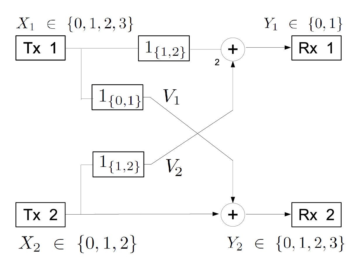
Refer to caption
Fig. 5: “Symmetric Clipper” of Section X-B

The channel input and output alphabets are 𝒳1={0,1,2,3}=𝒴2\mathcal{X}_{1}=\{0,1,2,3\}=\mathcal{Y}_{2}, 𝒳2∈{0,1,2}\mathcal{X}_{2}\in\{0,1,2\}, and 𝒴1={0,1}\mathcal{Y}_{1}=\{0,1\}. The input/output relationships are:

Y1=1{1,2}(X1)⊕21{1,2}(X2)Y2=1{0,1}​(X1)⊕X2\begin{array}[]{l l l l l l l l l l}Y_{1}=1_{\{1,2\}}(X_{1})\oplus_{2}1_{\{1,2\}}(X_{2})\\ Y_{2}=1_{\{0,1\}}(X_{1})\oplus X_{2}\end{array}

Consider the input distribution: Consider the input distribution:

P[X1=3]=1,X2∼𝒰⁡({1,2}),\begin{array}[]{l l l l l l l l l l}P[X_{1}=3]=1,\\ X_{2}\sim\mathcal{U}(\{1,2\}),\end{array}

in this case H⁡(Y1)=0H(Y_{1})=0 and H⁡(Y2)=1H(Y_{2})=1. This shows that there exists at least one input distribution for which H⁡(Y2)>H⁡(Y1)H(Y_{2})>H(Y_{1}) and thus this channel is not in the “very strong interference” regime. The outer bound of Theorem IX.1 is achieved here by a single input distribution pX1,X2p_{X_{1},X_{2}}: consider the distribution in Table III. This distribution produces H⁡(Y1)=1=log2⁡(|𝒴1|)H(Y_{1})=1=\log_{2}(|\mathcal{Y}_{1}|) and H⁡(Y2)=2=log⁡(|𝒴2|)H(Y_{2})=2=\log(|\mathcal{Y}_{2}|) and clearly no larger outer bound can exist given the output cardinality. We therefore conclude that the region of Theorem IX.1 can be rewritten as:

R1≤1R2≤2.\begin{array}[]{l l l l l l l l l l}R_{1}\leq 1\\ R_{2}\leq 2.\end{array}
TABLE III: The input distribution for Example II
X2X_{2} X1X_{1} 1 2 3 4
0 1/8 1/8 1/8 1/8 1/2
1 1/8 1/8 0 0 1/4
2 1/8 1/8 0 0 1/4
3/8 3/8 1/8 1/8

This region can be shown to be achievable using the transmission scheme described in Table IV.

TABLE IV: Achievability table for the rate point (R1,R2)=(1,2)(R_{1},R_{2})=(1,2) in Example II.
ω1\omega_{1} ω2\omega_{2} x1x_{1} x2x_{2} v1v_{1} v2v_{2} y1y_{1} y2y_{2}
0 0 0 3 0 0 0 0 0
1 0 1 0 0 1 0 0 1
2 0 2 1 1 1 1 0 2
3 0 3 1 2 1 1 0 3
4 1 0 2 0 0 0 1 0
5 1 1 1 0 1 0 1 1
6 1 2 0 1 1 1 1 2
7 1 3 0 2 1 1 1 3

The decoding is simply ω^i=Yi,i∈{1,2}.\hat{\omega}_{i}=Y_{i},\ i\in\{1,2\}. This transmission scheme achieves the proposed outer bound, thus showing capacity. The transmission scheme can be described as follows:

  • •

    encoder 2 transmits [x2−1]+[x_{2}-1]^{+};

  • •

    encoder 1 transmits the value X1X_{1} that simultaneously makes Y1=ω1Y_{1}=\omega_{1} and Y2=ω2Y_{2}=\omega_{2}. For each ω1\omega_{1} and ω2\omega_{2} such a value always exists because X2X_{2} takes on only three possible values;

  • •

    receivers 1 and  2 decode ω^1=Y1\hat{\omega}_{1}=Y_{1} and ω^2=Y2\hat{\omega}_{2}=Y_{2}.

This example is particularly interesting since both decoders obtain the transmitted symbol without suffering any interference from the other user. Here cognition allows the simultaneous cancelation of the interference at both decoders. Encoder 2 has only three codewords and relies on transmitter 1 to achieve its full rate of R2=2R_{2}=2. In fact encoder 1 is able to design its codebook to transmit two codewords for its decoder and still contribute to the rate of primary user by making the codewords corresponding to ω2={2,3}\omega_{2}=\{2,3\} distinguishable at the cognitive decoder.

This feature of the capacity achieving scheme is intriguing: the primary transmitter needs the support of the cognitive transmitter to achieve R2=2R_{2}=2 since its input alphabet has cardinality three. The transmitters optimally design their codebooks so to make the effect X1X_{1} on both outputs the desired one.

For example consider the transmission of ω2=2\omega_{2}=2 or 33 (lines 2,3,62,3,6 and 77). In this case transmitter 1 sends x1=0x_{1}=0 or x1=1x_{1}=1 to simultaneously influence both channel outputs so that both decoders receive the desired symbols. This simultaneous cancelation is possible due to the channel’s deterministic nature and the extra message knowledge at the cognitive transmitter.

XI Conclusion

In this paper we focused on the discrete memoryless cognitive interference channel and derived new inner and outer bounds, derived the capacity region for a class of “better cognitive decoding” channels, and obtained the capacity region for the semi-deterministic cognitive interference channel. We proposed a new outer bound using an idea originally devised for the broadcast channel in [30]. This outer bound does not involve auxiliary RVs and is thus more easily computable. Our outer bound is in general looser than the outer bound in [4] and they coincide in the “strong interference” regime of [6]. We also proposed a new inner bound that generalizes all other known achievable rate regions. In particular we showed the inclusion of the region of [31, 24]; it was previously unclear how the performance of the scheme in [31, 24] compared with that of other achievable rate regions. We determined capacity for a class of channels that we term the “better cognitive decoding” regime. The conditions defining this regime are looser than the “very weak interference condition” of [4] and the “very strong interference condition” of [6] and is the largest region where capacity is known. We also determined the capacity region for the class of semi-deterministic cognitive interference channels where the output at the cognitive receiver is a deterministic function of the channel inputs. Furthermore, for channels where both outputs are deterministic functions of the inputs, we showed the achievability of our new outer bound. This result shows that our outer bound, even though looser than the outer bound in [4], is tight for certain channels. The scheme that achieves capacity in the deterministic cognitive interference channel uses Gelf’and-Pinsker binning against the interference created at the primary receiver. This binning is performed by the cognitive encoder for the cognitive decoder. This feature of the transmission scheme was never known before to be capacity achieving. We conclude the paper by presenting two examples that show new interesting features of the capacity achieving scheme in the deterministic cognitive interference channel. Extensions of the results presented here to Gaussian channels will be presented in [32].

References

  • [1] M. Best, “The wireless revolution and universal access,” Trends in Telecommunications Reform, pp. 1–24, Sep. 2003.
  • [2] A. Goldsmith, S. Jafar, I. Maric, and S. Srinivasa, “Breaking spectrum gridlock with cognitive radios: An information theoretic perspective,” Proc. IEEE, 2009.
  • [3] N. Devroye, P. Mitran, and V. Tarokh, “Achievable rates in cognitive radio channels,” Information Theory, IEEE Transactions on, vol. 52, no. 5, pp. 1813–1827, May 2006.
  • [4] W. Wu, S. Vishwanath, and A. Arapostathis, “Capacity of a class of cognitive radio channels: Interference channels with degraded message sets,” Information Theory, IEEE Transactions on, vol. 53, no. 11, pp. 4391–4399, Nov. 2007.
  • [5] A. Jovicic and P. Viswanath, “Cognitive radio: An information-theoretic perspective,” Proc. IEEE Int. Symp. Inf. Theory, pp. 2413–2417, July 2006.
  • [6] I. Maric, R. Yates, and G. Kramer, “The capacity region of the strong interference channel with common information,” in The Thirty-Ninth Asilomar Conference on Signals, Systems and Computers, Nov. 2005, pp. 1737–1741.
  • [7] Y. Liang, A. Somekh-Baruch, H. V. Poor, S. Shamai, and S. Verdú, “Cognitive interference channels with confidential messages,” Proceedings of the 45th Annual Allerton Conference.
  • [8] I. Maric, A. J. Goldsmith, G. Kramer, and S. Shamai, “On the capacity of interference channels with one cooperating transmitter,” European Transactions on Telecommunications, vol. 19, no. 4, pp. 405–420, 2008.
  • [9] C. Nair and A. El Gamal, “An outer bound to the capacity region ofthe broadcast channel,” Information Theory, IEEE Transactions on, vol. 53, no. 1, pp. 350–355, Jan. 2007.
  • [10] Y. Cao and B. Chen, “Interference channel with one cognitive transmitter,” in Asilomar Conference on Signals, Systems, and Computers, 2008.
  • [11] I. Maric, R. Dabora, and A. Goldsmith, “On the capacity of the interference channel with a relay,” in Proc. IEEE Int. Symp. Inf. Theory (ISIT), 2008.
  • [12] I. Maric, R. Yates, and G. Kramer, “Capacity of interference channels with partial transmitter cooperation,” Information Theory, IEEE Transactions on, vol. 53, no. 10, pp. 3536–3548, Oct. 2007.
  • [13] D. Tuninetti, “The interference channels with generalized feedback,” in IEEE Proc. Int. Symp. Inf. Th., Nice, France, 2007.
  • [14] S. Seyedmehdi, Y. Xin, and Y. Lian, “An achievable rate region for the causal cognitive radio,” in Proc. Allerton Conf. Communications Control and Computer, 2007.
  • [15] D. Chatterjee, T. Wong, and O. Oyman, “Achievable rate in cognitive radio networks,” in Proc. Asilomar Conferenece on Signal, Systems and Computers, 2009.
  • [16] O. Sahin and E. Erkip, “On achievable rates for interference relay channel with interference cancelation,” Forty-First Asilomar Conference on Signals, Systems and Computers, 2007.
  • [17] S. Sridharan, S. Vishwanath, S. Jafar, and S. Shamai, “On the capacity of cognitive relay assisted gaussian interference channel,” in Proc. IEEE Int. Symp. Information Theory (ISIT) , Toronto, Canada, 2008, pp. 549–553.
  • [18] J. A. T. Thomas M. Cover, Elements of Information Theory. Wiley-Interscience, 1991.
  • [19] T. Han and K. Kobayashi, “A new achievable rate region for the interference channel,” Information Theory, IEEE Transactions on, vol. 27, no. 1, pp. 49–60, Jan 1981.
  • [20] J. Jiang and Y. Xin, “On the achievable rate regions for interference channels with degraded message sets,” Information Theory, IEEE Transactions on, vol. 54, no. 10, pp. 4707–4712, Oct. 2008.
  • [21] I. Maric, R. D. Yates, and G. Kramer, “The strong interference channel with unidirectional cooperation,” in The Information Theory and Applications (ITA) Inaugural Workshop, UCSD, La Jolla, Feb 2006.
  • [22] S. Gel’fand and M. Pinsker, “Coding for channel with random parameters,” Problems of control and information theory, 1980.
  • [23] K. Marton, “A coding theorem for the discrete memoryless broadcast channel,” Information Theory, IEEE Transactions on, vol. 25, no. 3, pp. 306–311, May 1979.
  • [24] N. Devroye, “Information theoretic limits of cognition and cooperation in wireless networks,” Ph.D. dissertation, Harvard University, 2007.
  • [25] J. Jiang, I. Maric, A. Goldsmith, and S. Cui, “Achievable Rate Regions for Broadcast Channels With Cognitive Relays,” in Proc. IEEE Information Theory Workshop (ITW), Taormina, Oct. 2009.
  • [26] Y. Cao and B. Chen, “Interference channels with one cognitive transmitter,” in Proc. Asilomar Conferenece on Signal, Systems and Computers, 2009.
  • [27] J. Jiang, Y. Xin, and H. Garg, “The capacity region of a class of deterministic interference channels with common information,” Acoustics, Speech and Signal Processing (ICASSP) , 2007. IEEE International Conference on, vol. 3, pp. III–681–III–684, April 2007.
  • [28] S. Lall, “Advanced topics in computation for control,” Lecture Notes for Engr. 210b at Stanford University, Stanford, CA, 2004.
  • [29] H. Chong, M. Motani, H. Garg, and H. Gamal, “On the Han-Kobayashi region for the interference channel,” IEEE Transactions on Information Theory, vol. 54, no. 7, pp. 3188–3194, 2008.
  • [30] H. Sato, “An outer bound to the capacity region of broadcast channels (Corresp.),” IEEE Transactions on Information Theory, vol. 24, no. 3, pp. 374–377, 1978.
  • [31] N. Devroye, P. Mitran, and V. Tarokh, “Cognitive multiple access networks,” in Proc. IEEE Int. Symp. Inf. Theory, 2005, pp. 57–61.
  • [32] S. Rini, D. Tuninetti, and N. Devroye, “New inner and outer bounds for the gaussian cognitive channel and some capacity results,” IEEE Transactions on Information Theory, 2010, to be submitted.
  • [33] F. Willems and E. Van der Meulen, “The discrete memoryless multiple-access channel with cribbing encoders,” IEEE Transactions on Information Theory, vol. 31, no. 3, pp. 313–327, 1985.

-A Error analysis of the achievable region ℛR​T​D\mathcal{R}_{RTD} of Theorem V.1

Without loss of generality assume that the message (w1​c,w2​c,w2​p​a,w1​p​b,w2​p​b)=(1,1,1,1,1)(w_{1c},w_{2c},w_{2pa},w_{1pb},w_{2pb})=(1,1,1,1,1) was sent and let (b¯0,b¯1,b¯2)(\overline{b}_{0},\overline{b}_{1},\overline{b}_{2}) be the tuple (b0,b1,b2)(b_{0},b_{1},b_{2}) chosen at encoder 1. Let (w^1​c,w^2​c,w^2​p​a,w^2​p​b,b^0,b^2)(\widehat{w}_{1c},\widehat{w}_{2c},\widehat{w}_{2pa},\widehat{w}_{2pb},\hat{b}_{0},\hat{b}_{2}) be the estimate at the decoder 2 and (w^^1​c,w^^2​c,w^^1​p​b,b^^0,b^^1)(\widehat{\widehat{w}}_{1c},\widehat{\widehat{w}}_{2c},\widehat{\widehat{w}}_{1pb},\hat{\hat{b}}_{0},\hat{\hat{b}}_{1}) be the estimate at the decoder 1.

The probability of error at decoder uu, u∈{1,2}u\in\{1,2\}, is bounded by

P⁡[error​u]≤P⁡[error​u|encoding​successful]+P⁡[encoding​NOT​successful].P[{\rm error}~u]\leq P[{\rm error}~u|{\rm encoding\,successful}]+P[{\rm encoding\,NOT\,successful}].

An encoding error occurs if encoder 1 is not able to find a tuple (b¯0,b¯1,b¯2)(\overline{b}_{0},\overline{b}_{1},\overline{b}_{2}) that guarantees typicality. A decoding error is committed at decoder 1 when (w^^1​c,w^^1​p​b)≠(1,1)(\widehat{\widehat{w}}_{1c},\widehat{\widehat{w}}_{1pb})\neq(1,1). A decoding error is committed at decoder 2 when (w^2​c,w^2​p​a,w^2​p​b)≠(1,1,1)(\widehat{w}_{2c},\widehat{w}_{2pa},\widehat{w}_{2pb})\neq(1,1,1).

-B Encoding Error

The probability that the encoding fails can be bounded as:

P[encodingNOTsuccessful]=P[⋂b0=12N​R1​c′⋂b1=12N​R1​p​b′⋂b2=12N​R2​p​b′(U2​cN(1),X2N(1,1),U1​cN(1,1,b0),U1​p​bN(1,1,b0,1,b1),U2​p​bN(1,1,b0,1,b2))∉TϵN(pU2​c,X2,U1​c,U1​p​b,U2​p​b)]=P[K=0]≤Var⁡[K]E2​[K]\begin{array}[]{l l l l l l l l l l}P[{\rm encoding\,NOT\,successful}]=P\left[\bigcap_{b_{0}=1}^{2^{NR^{\prime}_{1c}}}\bigcap_{b_{1}=1}^{2^{NR^{\prime}_{1pb}}}\bigcap_{b_{2}=1}^{2^{NR^{\prime}_{2pb}}}\right.\\ \ \ \ \ \ \left.\left(U_{2c}^{N}(1),X_{2}^{N}(1,1),U_{1c}^{N}(1,1,b_{0}),U_{1pb}^{N}(1,1,b_{0},1,b_{1}),U_{2pb}^{N}(1,1,b_{0},1,b_{2})\right)\notin T_{\epsilon}^{N}(p_{U_{2c},X_{2},U_{1c},U_{1pb},U_{2pb}})\right]\\ \ \ \ \ \ \ \ \ \ \ =P[K=0]\leq\frac{{\rm Var}[K]}{E^{2}[K]}\end{array}

where

K=∑b0=12N​R1​c′∑b1=12N​R1​p​b′∑b2=12N​R2​p​b′Kb0,b1,b2K=\sum_{b_{0}=1}^{2^{NR^{\prime}_{1c}}}\sum_{b_{1}=1}^{2^{NR^{\prime}_{1pb}}}\sum_{b_{2}=1}^{2^{NR^{\prime}_{2pb}}}K_{b_{0},b_{1},b_{2}}

and

Kb0,b1,b2=1{(U2​cN(1),X2N(1,1),U1​cN(1,1,b0),U1​p​bN(1,1,b0,1,b1),U2​p​bN(1,1,b0,1,b2))∈TϵN(pU2​c,X2,U1​c,U1​p​b,U2​p​b)},K_{b_{0},b_{1},b_{2}}=1_{\left\{\left(U_{2c}^{N}(1),X_{2}^{N}(1,1),U_{1c}^{N}(1,1,b_{0}),U_{1pb}^{N}(1,1,b_{0},1,b_{1}),U_{2pb}^{N}(1,1,b_{0},1,b_{2})\right)\in T_{\epsilon}^{N}(p_{U_{2c},X_{2},U_{1c},U_{1pb},U_{2pb}})\right\}},

where 1{x∈A}=11_{\{x\in A\}}=1 if x∈Ax\in A and zero otherwise.

The mean value of KK (neglecting all terms that depend on ϵ\epsilon and that eventually go to zero) is:

E[K]=∑b0=12N​R1​c′∑b1=12N​R1​p​b′∑b2=12N​R2​p​b′P[Kb0,b1,b2=1]=2N⁡(R1​c′+R1​p​b′+R2​p​b′−A)\displaystyle E[K]=\sum_{b_{0}=1}^{2^{NR^{\prime}_{1c}}}\sum_{b_{1}=1}^{2^{NR^{\prime}_{1pb}}}\sum_{b_{2}=1}^{2^{NR^{\prime}_{2pb}}}P[K_{b_{0},b_{1},b_{2}}=1]=2^{N(R^{\prime}_{1c}+R^{\prime}_{1pb}+R^{\prime}_{2pb}-A)}

with

2−N​A\displaystyle 2^{-NA} =P[Kb0,b1,b2=1]=E[Kb0,b1,b2]\displaystyle=P[K_{b_{0},b_{1},b_{2}}=1]=E[K_{b_{0},b_{1},b_{2}}]
=P[(U2​cN(1),X2N(1,1),U1​cN(1,1,b0),U1​p​bN(1,1,b0,1,b1),U2​p​bN(1,1,b0,1,b2))∈TϵN(pU2​c,X2,U1​c,U1​p​b,U2​p​b)]\displaystyle=P[\left(U_{2c}^{N}(1),X_{2}^{N}(1,1),U_{1c}^{N}(1,1,b_{0}),U_{1pb}^{N}(1,1,b_{0},1,b_{1}),U_{2pb}^{N}(1,1,b_{0},1,b_{2})\right)\in T_{\epsilon}^{N}(p_{U_{2c},X_{2},U_{1c},U_{1pb},U_{2pb}})]
=∑(u1​cN,u1​p​bN,u2​p​bN)∈TϵN​(pU2​c,X2,U1​c,U1​p​b,U2​p​b|u2​cN,x2N)pU1​c|U2​c​pU2​p​b|U2​c,U1​c,X2​pU1​p​b|U2​c,U1​c\displaystyle=\sum_{(u^{N}_{1c},u^{N}_{1pb},u^{N}_{2pb})\in T_{\epsilon}^{N}(p_{U_{2c},X_{2},U_{1c},U_{1pb},U_{2pb}}|u^{N}_{2c},x^{N}_{2})}p_{U_{1c}|U_{2c}}\,p_{U_{2pb}|U_{2c},U_{1c},X_{2}}\,p_{U_{1pb}|U_{2c},U_{1c}}
≥2−N[I(U1​c;X2|U2​c)+I(U1​p​b;X2,U2​p​b|U1​c,U2​c)].\displaystyle\geq 2^{-N[I(U_{1c};X_{2}|U_{2c})+I(U_{1pb};X_{2},U_{2pb}|U_{1c},U_{2c})]}.

The variance of KK (neglecting all terms that depend on ϵ\epsilon and that eventually go to zero) is:

Var⁡[K]\displaystyle{\rm Var}[K] =∑b0=12N​R1​c′∑b1=12N​R1​p​b′∑b2=12N​R2​p​b′∑b0′=12N​R1​c′∑b1′=12N​R1​p​b′∑b2′=12N​R2​p​b′(P[Kb0,b1,b2=1,Kb0′,b1′,b2′=1]−P[Kb0,b1,b2=1]P[Kb0′,b1′,b2′=1])\displaystyle=\sum_{b_{0}=1}^{2^{NR^{\prime}_{1c}}}\sum_{b_{1}=1}^{2^{NR^{\prime}_{1pb}}}\sum_{b_{2}=1}^{2^{NR^{\prime}_{2pb}}}\sum_{b_{0}^{\prime}=1}^{2^{NR^{\prime}_{1c}}}\sum_{b_{1}^{\prime}=1}^{2^{NR^{\prime}_{1pb}}}\sum_{b_{2}^{\prime}=1}^{2^{NR^{\prime}_{2pb}}}\left(P[K_{b_{0},b_{1},b_{2}}=1,K_{b^{\prime}_{0},b^{\prime}_{1},b^{\prime}_{2}}=1]-P[K_{b_{0},b_{1},b_{2}}=1]P[K_{b^{\prime}_{0},b^{\prime}_{1},b^{\prime}_{2}}=1]\right)
=∑b0′=b0,(b1,b2,b1′,b2′)(P[Kb0,b1,b2=1,Kb0,b1′,b2′=1]−P[Kb0,b1,b2=1]P[Kb0,b1′,b2′=1])\displaystyle=\sum_{b_{0}^{\prime}=b_{0},(b_{1},b_{2},b_{1}^{\prime},b_{2}^{\prime})}\left(P[K_{b_{0},b_{1},b_{2}}=1,K_{b_{0},b_{1}^{\prime},b_{2}^{\prime}}=1]-P[K_{b_{0},b_{1},b_{2}}=1]P[K_{b_{0},b_{1}^{\prime},b_{2}^{\prime}}=1]\right)
≤∑b0,(b1,b2,b1′,b2′)P⁡[Kb0,b1,b2=1,Kb0,b1′,b2′=1]\displaystyle\leq\sum_{b_{0},(b_{1},b_{2},b_{1}^{\prime},b_{2}^{\prime})}P[K_{b_{0},b_{1},b_{2}}=1,K_{b_{0},b_{1}^{\prime},b_{2}^{\prime}}=1]

because when b0≠b0′b_{0}\neq b_{0}^{\prime}, that is, U1​cN​(…,b0)U^{N}_{1c}(...,b_{0}) and U1​cN​(…,b0′)U^{N}_{1c}(...,b^{\prime}_{0}) are independent, the RVs Kb0,b1,b2K_{b_{0},b_{1},b_{2}} and Kb0′,b1′,b2′K_{b^{\prime}_{0},b_{1}^{\prime},b_{2}^{\prime}} are independent and they do not contribute to the summation. We thus can focus only on the case b0=b0′b_{0}=b_{0}^{\prime}. We can write:

Var⁡[K]\displaystyle{\rm Var}[K] ≤∑b0,b1=b1′,b2=b2′P[Kb0,b1,b2=1]⏟=E⁡[K]\displaystyle\leq\underbrace{\sum_{b_{0},\,b_{1}=b_{1}^{\prime},\,b_{2}=b_{2}^{\prime}}P[K_{b_{0},b_{1},b_{2}}=1]}_{=E[K]}
+∑b0,b1=b1′,b2≠b2′P[Kb0,b1,b2=1]P[Kb0,b1,b2′=1|Kb0,b1,b2=1]⏟=E⁡[K]​ 2N⁡(R2​p​b′−B)\displaystyle+\underbrace{\sum_{b_{0},\,b_{1}=b_{1}^{\prime},\,b_{2}\not=b_{2}^{\prime}}P[K_{b_{0},b_{1},b_{2}}=1]P[K_{b_{0},b_{1},b_{2}^{\prime}}=1|K_{b_{0},b_{1},b_{2}}=1]}_{=E[K]\,2^{N(R^{\prime}_{2pb}-B)}}
+∑b0,b1≠b1′,b2=b2′P[Kb0,b1,b2=1]P[Kb0,b1′,b2=1|Kb0,b1,b2=1]⏟=E⁡[K]​ 2N⁡(R1​p​b′−C)\displaystyle+\underbrace{\sum_{b_{0},\,b_{1}\not=b_{1}^{\prime},\,b_{2}=b_{2}^{\prime}}P[K_{b_{0},b_{1},b_{2}}=1]P[K_{b_{0},b_{1}^{\prime},b_{2}}=1|K_{b_{0},b_{1},b_{2}}=1]}_{=E[K]\,2^{N(R^{\prime}_{1pb}-C)}}
+∑b0,b1≠b1′,b2≠b2′P[Kb0,b1,b2=1]P[Kb0,b1′,b2′=1|Kb0,b1,b2=1]⏟=E⁡[K]​ 2N⁡(R1​p​b′+N​R2​p​b′−D)\displaystyle+\underbrace{\sum_{b_{0},\,b_{1}\not=b_{1}^{\prime},\,b_{2}\not=b_{2}^{\prime}}P[K_{b_{0},b_{1},b_{2}}=1]P[K_{b_{0},b_{1}^{\prime},b_{2}^{\prime}}=1|K_{b_{0},b_{1},b_{2}}=1]}_{=E[K]\,2^{N(R^{\prime}_{1pb}+NR^{\prime}_{2pb}-D)}}

and

2−N​B\displaystyle 2^{-NB} =P⁡[Kb0,b1,b2′=1|Kb0,b1,b2=1]\displaystyle=P[K_{b_{0},b_{1},b_{2}^{\prime}}=1|K_{b_{0},b_{1},b_{2}}=1]
=P[(U2​cN(1),X2N(1,1),U1​cN(1,1,b0),U1​p​bN(1,1,b0,1,b1),U2​p​bN(1,1,b0,1,b2′))∈TϵN(pU2​c,X2,U1​c,U1​p​b,U2​p​b)|\displaystyle=P[\left(U_{2c}^{N}(1),X_{2}^{N}(1,1),U_{1c}^{N}(1,1,b_{0}),U_{1pb}^{N}(1,1,b_{0},1,b_{1}),U_{2pb}^{N}(1,1,b_{0},1,b_{2}^{\prime})\right)\in T_{\epsilon}^{N}(p_{U_{2c},X_{2},U_{1c},U_{1pb},U_{2pb}})|
(U2​cN(1),X2N(1,1),U1​cN(1,1,b0),U1​p​bN(1,1,b0,1,b1),U2​p​bN(1,1,b0,1,b2))∈TϵN(pU2​c,X2,U1​c,U1​p​b,U2​p​b)]\displaystyle\qquad\left(U_{2c}^{N}(1),X_{2}^{N}(1,1),U_{1c}^{N}(1,1,b_{0}),U_{1pb}^{N}(1,1,b_{0},1,b_{1}),U_{2pb}^{N}(1,1,b_{0},1,b_{2})\right)\in T_{\epsilon}^{N}(p_{U_{2c},X_{2},U_{1c},U_{1pb},U_{2pb}})]
=∑u2​p​bN∈TϵN​(pU2​c,X2,U1​c,U1​p​b,U2​p​b|u2​cN,x2N,u1​cN,u1​p​bN)pU2​p​b|U2​c,U1​c,X2\displaystyle=\sum_{u^{N}_{2pb}\in T_{\epsilon}^{N}(p_{U_{2c},X_{2},U_{1c},U_{1pb},U_{2pb}}|u^{N}_{2c},x^{N}_{2},u^{N}_{1c},u^{N}_{1pb})}p_{U_{2pb}|U_{2c},U_{1c},X_{2}}
=2−NI(U2​p​b;U1​p​b|U2​c,U1​c,X2),\displaystyle=2^{-NI(U_{2pb};U_{1pb}|U_{2c},U_{1c},X_{2})},

and

2−N​C\displaystyle 2^{-NC} =P⁡[Kb0,b1′,b2=1|Kb0,b1,b2=1]\displaystyle=P[K_{b_{0},b_{1}^{\prime},b_{2}}=1|K_{b_{0},b_{1},b_{2}}=1]
=P[(U2​cN(1),X2N(1,1),U1​cN(1,1,b0),U1​p​bN(1,1,b0,1,b1′),U2​p​bN(1,1,b0,1,b2))∈TϵN(pU2​c,X2,U1​c,U1​p​b,U2​p​b)|\displaystyle=P[\left(U_{2c}^{N}(1),X_{2}^{N}(1,1),U_{1c}^{N}(1,1,b_{0}),U_{1pb}^{N}(1,1,b_{0},1,b_{1}^{\prime}),U_{2pb}^{N}(1,1,b_{0},1,b_{2})\right)\in T_{\epsilon}^{N}(p_{U_{2c},X_{2},U_{1c},U_{1pb},U_{2pb}})|
(U2​cN(1),X2N(1,1),U1​cN(1,1,b0),U1​p​bN(1,1,b0,1,b1),U2​p​bN(1,1,b0,1,b2))∈TϵN(pU2​c,X2,U1​c,U1​p​b,U2​p​b)]\displaystyle\qquad\left(U_{2c}^{N}(1),X_{2}^{N}(1,1),U_{1c}^{N}(1,1,b_{0}),U_{1pb}^{N}(1,1,b_{0},1,b_{1}),U_{2pb}^{N}(1,1,b_{0},1,b_{2})\right)\in T_{\epsilon}^{N}(p_{U_{2c},X_{2},U_{1c},U_{1pb},U_{2pb}})]
=∑u1​p​bN∈TϵN​(pU2​c,X2,U1​c,U1​p​b,U2​p​b|u2​cN,x2N,u1​cN,u2​p​bN)pU1​p​b|U2​c,U1​c\displaystyle=\sum_{u^{N}_{1pb}\in T_{\epsilon}^{N}(p_{U_{2c},X_{2},U_{1c},U_{1pb},U_{2pb}}|u^{N}_{2c},x^{N}_{2},u^{N}_{1c},u^{N}_{2pb})}p_{U_{1pb}|U_{2c},U_{1c}}
=2−NI(U1​p​b;X2,U2​p​b|U1​c,U2​c),\displaystyle=2^{-NI(U_{1pb};X_{2},U_{2pb}|U_{1c},U_{2c})},

and

2−N​D\displaystyle 2^{-ND} =P⁡[Kb0,b1′,b2′=1|Kb0,b1,b2=1]\displaystyle=P[K_{b_{0},b_{1}^{\prime},b_{2}^{\prime}}=1|K_{b_{0},b_{1},b_{2}}=1]
=P[(U2​cN(1),X2N(1,1),U1​cN(1,1,b0),U1​p​bN(1,1,b0,1,b1′),U2​p​bN(1,1,b0,1,b2′))∈TϵN(pU2​c,X2,U1​c,U1​p​b,U2​p​b)|\displaystyle=P[\left(U_{2c}^{N}(1),X_{2}^{N}(1,1),U_{1c}^{N}(1,1,b_{0}),U_{1pb}^{N}(1,1,b_{0},1,b_{1}^{\prime}),U_{2pb}^{N}(1,1,b_{0},1,b_{2}^{\prime})\right)\in T_{\epsilon}^{N}(p_{U_{2c},X_{2},U_{1c},U_{1pb},U_{2pb}})|
(U2​cN(1),X2N(1,1),U1​cN(1,1,b0),U1​p​bN(1,1,b0,1,b1),U2​p​bN(1,1,b0,1,b2))∈TϵN(pU2​c,X2,U1​c,U1​p​b,U2​p​b)]\displaystyle\qquad\left(U_{2c}^{N}(1),X_{2}^{N}(1,1),U_{1c}^{N}(1,1,b_{0}),U_{1pb}^{N}(1,1,b_{0},1,b_{1}),U_{2pb}^{N}(1,1,b_{0},1,b_{2})\right)\in T_{\epsilon}^{N}(p_{U_{2c},X_{2},U_{1c},U_{1pb},U_{2pb}})]
=∑(u1​p​bN,u2​p​bN)∈TϵN​(pU2​c,X2,U1​c,U1​p​b,U2​p​b|u2​cN,x2N,u1​cN)pU2​p​b|U2​c,U1​c,X2​pU1​p​b|U2​c,U1​c\displaystyle=\sum_{(u^{N}_{1pb},u^{N}_{2pb})\in T_{\epsilon}^{N}(p_{U_{2c},X_{2},U_{1c},U_{1pb},U_{2pb}}|u^{N}_{2c},x^{N}_{2},u^{N}_{1c})}p_{U_{2pb}|U_{2c},U_{1c},X_{2}}\,p_{U_{1pb}|U_{2c},U_{1c}}
=2−NI(U1​p​b;X2,U2​p​b|U1​c,U2​c)=2−N​C.\displaystyle=2^{-NI(U_{1pb};X_{2},U_{2pb}|U_{1c},U_{2c})}=2^{-NC}.

Hence, we can bound P[K=0]P[K=0] as:

0≤P[K=0]≤1+2N⁡(R1​p​b′−C)+2N⁡(R2​p​b′−B)+2N⁡(R1​p​b′+R2​p​b′−C)2N⁡(R1​c′+R1​p​b′+R2​p​b′−I⁡(U1​c;X2|U2​c)−C)\begin{array}[]{l l l l l l l l l l}0\leq P[K=0]&\leq\displaystyle\frac{1+2^{N(R^{\prime}_{1pb}-C)}+2^{N(R^{\prime}_{2pb}-B)}+2^{N(R^{\prime}_{1pb}+R^{\prime}_{2pb}-C)}}{2^{N(R^{\prime}_{1c}+R^{\prime}_{1pb}+R^{\prime}_{2pb}-I(U_{1c};X_{2}|U_{2c})-C)}}\end{array}

and P[K=0]→0P[K=0]\to 0 if

R1​c′+R1​p​b′+R2​p​b′−I⁡(U1​c;X2|U2​c)−C>0\displaystyle R^{\prime}_{1c}+R^{\prime}_{1pb}+R^{\prime}_{2pb}-I(U_{1c};X_{2}|U_{2c})-C>0
R1​c′+R1​p​b′+R2​p​b′−I⁡(U1​c;X2|U2​c)−C−(R2​p​b′−B)>0\displaystyle R^{\prime}_{1c}+R^{\prime}_{1pb}+R^{\prime}_{2pb}-I(U_{1c};X_{2}|U_{2c})-C-(R^{\prime}_{2pb}-B)>0
R1​c′+R1​p​b′+R2​p​b′−I⁡(U1​c;X2|U2​c)−C−(R1​p​b′−C)>0\displaystyle R^{\prime}_{1c}+R^{\prime}_{1pb}+R^{\prime}_{2pb}-I(U_{1c};X_{2}|U_{2c})-C-(R^{\prime}_{1pb}-C)>0
R1​c′+R1​p​b′+R2​p​b′−I⁡(U1​c;X2|U2​c)−C−(R1​p​b′+R2​p​b′−C)>0\displaystyle R^{\prime}_{1c}+R^{\prime}_{1pb}+R^{\prime}_{2pb}-I(U_{1c};X_{2}|U_{2c})-C-(R^{\prime}_{1pb}+R^{\prime}_{2pb}-C)>0

that is, if

R1​c′+R1​p​b′+R2​p​b′\displaystyle R^{\prime}_{1c}+R^{\prime}_{1pb}+R^{\prime}_{2pb} >I(U1​c;X2|U2​c)+I(U1​p​b;X2,U2​p​b|U1​c,U2​c)\displaystyle>I(U_{1c};X_{2}|U_{2c})+I(U_{1pb};X_{2},U_{2pb}|U_{1c},U_{2c})
=I(U1​c,U1​p​b;X2|U2​c)+I(U1​p​b;U2​p​b|U1​c,U2​c,X2)\displaystyle=I(U_{1c},U_{1pb};X_{2}|U_{2c})+I(U_{1pb};U_{2pb}|U_{1c},U_{2c},X_{2})
R1​c′+R1​p​b′\displaystyle R^{\prime}_{1c}+R^{\prime}_{1pb} >I(U1​c;X2|U2​c)+I(U1​p​b;X2|U1​c,U2​c)\displaystyle>I(U_{1c};X_{2}|U_{2c})+I(U_{1pb};X_{2}|U_{1c},U_{2c})
=I⁡(U1​c,U1​p​b;X2|U2​c)\displaystyle=I(U_{1c},U_{1pb};X_{2}|U_{2c})
R1​c′+R2​p​b′\displaystyle R^{\prime}_{1c}+R^{\prime}_{2pb} >I⁡(U1​c;X2|U2​c),\displaystyle>I(U_{1c};X_{2}|U_{2c}),
R1​c′\displaystyle R^{\prime}_{1c} >I⁡(U1​c;X2|U2​c)\displaystyle>I(U_{1c};X_{2}|U_{2c})

as in (12a)-(12c), because the second to last equation is redundant.

-C Decoding Errors at decoder 2

TABLE V: Error events at decoder 2.
Event w2​cw_{2c} (w1​c,b1)(w_{1c},b_{1}) w2​p​aw_{2pa} w2​p​bw_{2pb} pY2|⋆p_{Y_{2}|\star}
E2,1E_{2,1} X ⋯\cdots ⋯\cdots ⋯\cdots pY2p_{Y_{2}}
E2,2​aE_{2,2a} 1 X X ⋯\cdots pY2|U2​cp_{Y_{2}|U_{2c}}
E2,2​bE_{2,2b} 1 1 X ⋯\cdots pY2|U2​c,U1​cp_{Y_{2}|U_{2c},U_{1c}}
E2,3​aE_{2,3a} 1 X 1 X pY2|U2​c,X2p_{Y_{2}|U_{2c},X_{2}}
E2,3​bE_{2,3b} 1 1 1 X PY2|U2​c,U1​c,X2P_{Y_{2}|U_{2c},U_{1c},X_{2}}

If decoder 2 decodes (w^2​c,w^2​p​a,w^2​p​b)≠(1,1,1)(\widehat{w}_{2c},\widehat{w}_{2pa},\widehat{w}_{2pb})\not=(1,1,1), then an error is committed. The probability of error at decoder 2 is bounded as:

P⁡[error​2|encoding​successful]≤∑i∈{1,2​a,2​b,3​a,3​b}P⁡[E2,i],P[{\rm error}~2|{\rm encoding\,successful}]\leq\sum_{i\in\{1,2a,2b,3a,3b\}}P[E_{2,i}],

where E2,iE_{2,i}, i∈{1,2​a,2​b,3​a,3​b}i\in\{1,2a,2b,3a,3b\}, are the error events defined in Table V. In Table V, an “X” means that the corresponding message is in error (when the header of the column contains two indices, an “X” indicates that at least one of the two indexes is wrong), a “1” means that the corresponding message is correct, while the dots “⋯\cdots” indicates that “it does not matter whether the corresponding message is correct or not; in this case the most restrictive case is when the message is actually wrong.” The last column of Table V specifies the pY2|⋆p_{Y_{2}|\star} to be used in (15).

We have that P⁡[error​2|encoding​successful]→0P[{\rm error}~2|{\rm encoding\,successful}]\to 0 when N→∞N\rightarrow\infty if:

  • •

    When the event E2,1E_{2,1} occurs we have w^2​c≠1\widehat{w}_{2c}\neq 1. In this case the received Y2NY_{2}^{N} is independent of the transmitted sequences. This follows from the fact that the codewords U2​cNU_{2c}^{N} are generated in an iid fashion and all the other codewords are generated independently conditioned on U2​cNU_{2c}^{N}. Hence, when decoder 2 finds a wrong U2​cNU_{2c}^{N}, all the decoded codewords are independent of the transmitted ones. We can bound the error probability of E2,1E_{2,1} as:

    P[E2,1]=P[⋃w~2​c≠1,w~2​p​a,w~1​c,w~2​p​b,b0,b2\displaystyle P[E_{2,1}]=P\left[\bigcup_{\widetilde{w}_{2c}\neq 1,\widetilde{w}_{2pa},\widetilde{w}_{1c},\widetilde{w}_{2pb},b_{0},b_{2}}\right.
    (Y2N,U2​cN(w~2​c),U1​cN(w~1​c,w~2​c,b0),X2N(w~2​c,w~2​p​a),U2​p​bN(w~2​c,w~2​p​a,w~1​c,b0,w~2​p​b,b2))∈TϵN(pY2,U2​c,U1​c,X2,U2​p​b)]\displaystyle\left.(Y_{2}^{N},U_{2c}^{N}(\widetilde{w}_{2c}),U_{1c}^{N}(\widetilde{w}_{1c},\widetilde{w}_{2c},b_{0}),X_{2}^{N}(\widetilde{w}_{2c},\widetilde{w}_{2pa}),U_{2pb}^{N}(\widetilde{w}_{2c},\widetilde{w}_{2pa},\widetilde{w}_{1c},b_{0},\widetilde{w}_{2pb},b_{2}))\in T_{\epsilon}^{N}\left(p_{Y_{2},U_{2c},U_{1c},X_{2},U_{2pb}}\right)\right]
    ≤2N⁡(R2​c+R2​p​a+R1​c+R1​c′+R2​p​b+R2​p​b′)​∑(y2N,u2​cN,u1​cN,x2N,u2​p​bN)∈TϵN​(pY2,U2​c,U1​c,X2,U2​p​b)p2|⋆|⋆=∅\displaystyle\leq 2^{N(R_{2c}+R_{2pa}+R_{1c}+R^{\prime}_{1c}+R_{2pb}+R^{\prime}_{2pb})}\sum_{(y_{2}^{N},u^{N}_{2c},u^{N}_{1c},x^{N}_{2},u^{N}_{2pb})\in T_{\epsilon}^{N}\left(p_{Y_{2},U_{2c},U_{1c},X_{2},U_{2pb}}\right)}p_{2|\star}|_{\star=\emptyset}
    ≤2N⁡(R2​c+R2​p​a+R1​c+R1​c′+R2​p​b+R2​p​b′−I2|⋆|⋆=∅)\displaystyle\leq 2^{N(R_{2c}+R_{2pa}+R_{1c}+R^{\prime}_{1c}+R_{2pb}+R^{\prime}_{2pb}-I_{2|\star}|_{\star=\emptyset})}

    for p2|⋆p_{2|\star} given in (16) and I2|⋆I_{2|\star} given in (17). Hence P⁡[E2,1]→0P[E_{2,1}]\to 0 as N→∞N\rightarrow\infty if (12d) is satisfied.

  • •

    When the event E2,2E_{2,2} occurs, i.e., either E2,2​aE_{2,2a} or E2,2​bE_{2,2b}, we have w^2​c=1\widehat{w}_{2c}=1 but w^2​p​a≠1\widehat{w}_{2pa}\neq 1. Whether w^1​c\widehat{w}_{1c} is correct or not, it does not matter since decoder 2 is not interested in w^1​c\widehat{w}_{1c}. However we need to consider whether the pair (w^1​c,b^0)(\widehat{w}_{1c},\widehat{b}_{0}) is equal to the transmitted one or not because this affects the way the joint probability among all involved RVs factorizes. We have:

    • –

      Case E2,2​aE_{2,2a}: either w^1​c≠1\widehat{w}_{1c}\neq 1 or b^0≠b¯0\widehat{b}_{0}\neq\overline{b}_{0}. In this case, conditioned on the (correct) decoded sequence U2​cNU_{2c}^{N}, the output Y2NY_{2}^{N} is independent of the (wrong) decoded sequences U1​cNU_{1c}^{N}, X2NX_{2}^{N} and also of U2​p​bNU_{2pb}^{N} (because U2​p​bNU_{2pb}^{N} is superimposed to the wrong pair (U1​cN,X2N)(U_{1c}^{N},X_{2}^{N})). It is easy to see that the most stringent error event is when both w^1​c≠1\widehat{w}_{1c}\neq 1 and b^0≠b¯0\widehat{b}_{0}\neq\overline{b}_{0}. Thus we have

      P[E2,2​a]=P[⋃w~2​p​a≠1,w~1​c≠1,b0≠b¯0,w~2​p​b,b2\displaystyle P[E_{2,2a}]=P\left[\bigcup_{\widetilde{w}_{2pa}\neq 1,\widetilde{w}_{1c}\neq 1,b_{0}\neq\overline{b}_{0},\widetilde{w}_{2pb},b_{2}}\right.
      (Y2N,U2​cN(1),U1​cN(1,w~1​c,b0),X2N(1,w~2​p​a),U2​p​bN(1,w~2​p​a,w~1​c,b0,w~2​p​b,b2))∈TϵN(pY2,U2​c,U1​c,X2,U2​p​b)]\displaystyle\left.(Y_{2}^{N},U_{2c}^{N}(1),U_{1c}^{N}(1,\widetilde{w}_{1c},b_{0}),X_{2}^{N}(1,\widetilde{w}_{2pa}),U_{2pb}^{N}(1,\widetilde{w}_{2pa},\widetilde{w}_{1c},b_{0},\widetilde{w}_{2pb},b_{2}))\in T_{\epsilon}^{N}\left(p_{Y_{2},U_{2c},U_{1c},X_{2},U_{2pb}}\right)\right]
      ≤2N⁡(R2​p​a+R1​c+R1​c′+R2​p​b+R2​p​b′)​∑(y2N,u2​cN,u1​cN,x2N,u2​p​bN)∈TϵN​(pY2,U2​c,U1​c,X2,U2​p​b)p2|⋆|⋆=U2​c\displaystyle\leq 2^{N(R_{2pa}+R_{1c}+R^{\prime}_{1c}+R_{2pb}+R^{\prime}_{2pb})}\sum_{(y_{2}^{N},u^{N}_{2c},u^{N}_{1c},x^{N}_{2},u^{N}_{2pb})\in T_{\epsilon}^{N}\left(p_{Y_{2},U_{2c},U_{1c},X_{2},U_{2pb}}\right)}p_{2|\star}|_{\star=U_{2c}}
      ≤2N⁡(R2​p​a+R1​c+R1​c′+R2​p​b+R2​p​b′−I2|⋆|⋆=U2​c)\displaystyle\leq 2^{N(R_{2pa}+R_{1c}+R^{\prime}_{1c}+R_{2pb}+R^{\prime}_{2pb}-I_{2|\star}|_{\star=U_{2c}})}

      for p2|⋆p_{2|\star} given in (16) and I2|⋆I_{2|\star} given in (17). Hence P⁡[E2,2​a]→0P[E_{2,2a}]\to 0 as N→∞N\rightarrow\infty if (12e) is satisfied.

    • –

      Case E2,2​bE_{2,2b}: both w^1​c=1\widehat{w}_{1c}=1 and b^0=b¯0\widehat{b}_{0}=\overline{b}_{0}. In this case, conditioned on the (correct) decoded (U2​cN,U1​cN)(U_{2c}^{N},U_{1c}^{N}), the output Y2NY_{2}^{N} is independent of the (wrong) decoded sequences (X2N,U2​p​bN)(X_{2}^{N},U_{2pb}^{N}). Thus we have

      P[E2,2​b]=P[⋃w~2​p​a≠1,w~2​p​b,b2\displaystyle P[E_{2,2b}]=P\left[\bigcup_{\widetilde{w}_{2pa}\neq 1,\widetilde{w}_{2pb},b_{2}}\right.
      (Y2N,U2​cN(1),U1​cN(1,1,b¯0),X2N(1,w~2​p​a),U2​p​bN(1,w~2​p​a,1,b¯0,w~2​p​b,b2))∈TϵN(pY2,U2​c,U1​c,X2,U2​p​b)]\displaystyle\left.(Y_{2}^{N},U_{2c}^{N}(1),U_{1c}^{N}(1,1,\overline{b}_{0}),X_{2}^{N}(1,\widetilde{w}_{2pa}),U_{2pb}^{N}(1,\widetilde{w}_{2pa},1,\overline{b}_{0},\widetilde{w}_{2pb},b_{2}))\in T_{\epsilon}^{N}\left(p_{Y_{2},U_{2c},U_{1c},X_{2},U_{2pb}}\right)\right]
      ≤2N⁡(R2​p​a+R2​p​b+R2​p​b′)​∑(y2N,u2​cN,u1​cN,x2N,u2​p​bN)∈TϵN​(pY2,U2​c,U1​c,X2,U2​p​b)p2|⋆|⋆=(U2​c,U1​c)\displaystyle\leq 2^{N(R_{2pa}+R_{2pb}+R^{\prime}_{2pb})}\sum_{(y_{2}^{N},u^{N}_{2c},u^{N}_{1c},x^{N}_{2},u^{N}_{2pb})\in T_{\epsilon}^{N}\left(p_{Y_{2},U_{2c},U_{1c},X_{2},U_{2pb}}\right)}p_{2|\star}|_{\star=(U_{2c},U_{1c})}
      ≤2N⁡(R2​p​a+R2​p​b+R2​p​b′−I2|⋆|⋆=(U2​c,U1​c))\displaystyle\leq 2^{N(R_{2pa}+R_{2pb}+R^{\prime}_{2pb}-I_{2|\star}|_{\star=(U_{2c},U_{1c})})}

      for p2|⋆p_{2|\star} given in (16) and I2|⋆I_{2|\star} given in (17). Hence P⁡[E2,2​b]→0P[E_{2,2b}]\to 0 as N→∞N\rightarrow\infty if (12f) is satisfied.

  • •

    When the event E2,3E_{2,3} occurs, i.e., either E2,3​aE_{2,3a} or E2,3​bE_{2,3b}, we have w^2​c=1\widehat{w}_{2c}=1,w^2​p​a=1\widehat{w}_{2pa}=1 but w^2​p​b≠1\widehat{w}_{2pb}\neq 1. Again, whether w^1​c\widehat{w}_{1c} is correct or not, it does not matter since decoder 2 is not interested in w^1​c\widehat{w}_{1c}. However we need to consider whether the pair (w^1​c,b^0)(\widehat{w}_{1c},\widehat{b}_{0}) is equal to the transmitted one or not because this affects the way the joint probability among all involved RVs factorizes. The analysis proceeds as for the event E2,2E_{2,2}.

    We have:

    • –

      Case E2,3​aE_{2,3a}: either w^1​c≠1\widehat{w}_{1c}\neq 1 or b^0≠b¯0\widehat{b}_{0}\neq\overline{b}_{0}. In this case, conditioned on the (correct) decoded sequences (U2​cN,X2N)(U_{2c}^{N},X_{2}^{N}), the output Y2NY_{2}^{N} is independent of the (wrong) decoded sequences (U1​cN,U2​cn​U2​p​bN)(U_{1c}^{N},U_{2c}^{n}U_{2pb}^{N}). It is easy to see that the most stringent error event is when both w^1​c≠1\widehat{w}_{1c}\neq 1 and b^0≠b¯0\widehat{b}_{0}\neq\overline{b}_{0}. Thus we have

      P[E2,3​a]=P[⋃w~1​c≠1,b0≠b¯0,w~2​p​b,b2\displaystyle P[E_{2,3a}]=P\left[\bigcup_{\widetilde{w}_{1c}\neq 1,b_{0}\neq\overline{b}_{0},\widetilde{w}_{2pb},b_{2}}\right.
      (Y2N,U2​cN(1),U1​cN(1,w~1​c,b0),X2N(1,1),U2​p​bN(1,1,w~1​c,b0,w~2​p​b,b2))∈TϵN(pY2,U2​c,U1​c,X2,U2​p​b)]\displaystyle\left.(Y_{2}^{N},U_{2c}^{N}(1),U_{1c}^{N}(1,\widetilde{w}_{1c},b_{0}),X_{2}^{N}(1,1),U_{2pb}^{N}(1,1,\widetilde{w}_{1c},b_{0},\widetilde{w}_{2pb},b_{2}))\in T_{\epsilon}^{N}\left(p_{Y_{2},U_{2c},U_{1c},X_{2},U_{2pb}}\right)\right]
      ≤2N⁡(R1​c+R1​c′+R2​p​b+R2​p​b′)​∑(y2N,u2​cN,u1​cN,x2N,u2​p​bN)∈TϵN​(pY2,U2​c,U1​c,X2,U2​p​b)p2|⋆|⋆=(U2​c,X2)\displaystyle\leq 2^{N(R_{1c}+R^{\prime}_{1c}+R_{2pb}+R^{\prime}_{2pb})}\sum_{(y_{2}^{N},u^{N}_{2c},u^{N}_{1c},x^{N}_{2},u^{N}_{2pb})\in T_{\epsilon}^{N}\left(p_{Y_{2},U_{2c},U_{1c},X_{2},U_{2pb}}\right)}p_{2|\star}|_{\star=(U_{2c},X_{2})}
      ≤2N⁡(R2​p​a+R1​c+R1​c′+R2​p​b+R2​p​b′−I2|⋆|⋆=(U2​c,X2))\displaystyle\leq 2^{N(R_{2pa}+R_{1c}+R^{\prime}_{1c}+R_{2pb}+R^{\prime}_{2pb}-I_{2|\star}|_{\star=(U_{2c},X_{2})})}

      for p2|⋆p_{2|\star} given in (16) and I2|⋆I_{2|\star} given in (17). Hence P⁡[E2,3​a]→0P[E_{2,3a}]\to 0 as N→∞N\rightarrow\infty if (12g) is satisfied.

    • –

      Case E2,3​bE_{2,3b}: both w^1​c=1\widehat{w}_{1c}=1 and b^0=b¯0\widehat{b}_{0}=\overline{b}_{0}. In this case, conditioned on the (correct) decoded sequences (U2​cN,X2N,U1​cN)(U_{2c}^{N},X_{2}^{N},U_{1c}^{N}), the output Y2NY_{2}^{N} is independent of the (wrong) decoded sequence U2​p​bNU_{2pb}^{N}. However, since (U2​cN,X2N,U1​cN)(U_{2c}^{N},X_{2}^{N},U_{1c}^{N}) is the triplet that passed the encoding binning step, they are jointly typical. Hence, in this case we cannot use the factorization in p2|⋆p_{2|\star} given in (16), but we need to replace pU1​c|U2​cp_{U_{1c}|U_{2c}} in (16) with pU1​c|U2​c,X2p_{U_{1c}|U_{2c},X_{2}}. Thus we have

      P[E2,3​b]=P[⋃w~2​p​b,b2\displaystyle P[E_{2,3b}]=P\left[\bigcup_{\widetilde{w}_{2pb},b_{2}}\right.
      (Y2N,U2​cN(1),U1​cN(1,1,b¯0),X2N(1,1),U2​p​bN(1,1,1,b¯0,w~2​p​b,b2))∈TϵN(pY2,U2​c,U1​c,X2,U2​p​b)]\displaystyle\left.(Y_{2}^{N},U_{2c}^{N}(1),U_{1c}^{N}(1,1,\overline{b}_{0}),X_{2}^{N}(1,1),U_{2pb}^{N}(1,1,1,\overline{b}_{0},\widetilde{w}_{2pb},b_{2}))\in T_{\epsilon}^{N}\left(p_{Y_{2},U_{2c},U_{1c},X_{2},U_{2pb}}\right)\right]
      ≤2N⁡(R2​p​b+R2​p​b′)​∑(y2N,u2​cN,u1​cN,x2N,u2​p​bN)∈TϵN​(pY2,U2​c,U1​c,X2,U2​p​b)pU2​c​pX2|U2​c​pU1​c|U2​c,X2​pU2​p​b|U2​c,U1​c,X2​pY2|U1​c,U2​c,X2\displaystyle\leq 2^{N(R_{2pb}+R^{\prime}_{2pb})}\sum_{(y_{2}^{N},u^{N}_{2c},u^{N}_{1c},x^{N}_{2},u^{N}_{2pb})\in T_{\epsilon}^{N}\left(p_{Y_{2},U_{2c},U_{1c},X_{2},U_{2pb}}\right)}p_{U_{2c}}\,p_{X_{2}|U_{2c}}\,p_{U_{1c}|U_{2c},X_{2}}\,p_{U_{2pb}|U_{2c},U_{1c},X_{2}}\,p_{Y_{2}|U_{1c},U_{2c},X_{2}}
      ≤2N(R2​p​b+R′2​p​b−I(Y2;U2​p​b|U1​c,U2​c,X2))\displaystyle\leq 2^{N(R_{2pb}+R^{\prime}_{2pb}-I(Y_{2};U_{2pb}|U_{1c},U_{2c},X_{2}))}

      Hence P⁡[E2,3​b]→0P[E_{2,3b}]\to 0 as N→∞N\rightarrow\infty if (12h) is satisfied.

-D Decoding Errors at Decoder 1

TABLE VI: Error events at decoder 1.
Event w2​cw_{2c} (w1​c,b1)(w_{1c},b_{1}) w1​p​bw_{1pb} pY1|⋆p_{Y_{1}|\star}
E1,1E_{1,1} X ⋯\cdots ⋯\cdots pY1p_{Y_{1}}
E1,2E_{1,2} 1 X ⋯\cdots pY1|U2​cp_{Y_{1}|U_{2c}}
E1,3E_{1,3} 1 1 X PY1|U2​c,U1​cP_{Y_{1}|U_{2c},U_{1c}}

The probability of error at decoder 1 is bounded as:

P⁡[error​1|encoding​successful]≤∑i=13P⁡[E1,i],P[{\rm error}~1|{\rm encoding\,successful}]\leq\sum_{i=1}^{3}P[E_{1,i}],

where P⁡[E1,i]P[E_{1,i}] is the error event defined in Table VI. The meaning of the symbols in Table VI is as for Table V. We have that P⁡[error​1|encoding​successful]→0P[{\rm error}~1|{\rm encoding\,successful}]\to 0 when N→∞N\rightarrow\infty if:

  • •

    When the event E1,1E_{1,1} occurs we have w^2​c≠1\widehat{w}_{2c}\neq 1. In this case the received Y1NY_{1}^{N} is independent of the transmitted sequences. We can bound the error probability of E1,1E_{1,1} as:

    P[E1,1]=P[⋃w~2​c≠1,w~1​c,w~1​p​b,b0,b1\displaystyle P[E_{1,1}]=P\left[\bigcup_{\widetilde{w}_{2c}\neq 1,\widetilde{w}_{1c},\widetilde{w}_{1pb},b_{0},b_{1}}\right.
    (Y1N,U2​cN(w~2​c),U1​cN(w~1​c,w~2​c,b0),U1​p​bN(w~2​c,w~2​p​a,w~1​c,b0,w~2​p​b,b1))∈TϵN(pY1,U2​c,U1​c,U1​p​b)]\displaystyle\left.(Y_{1}^{N},U_{2c}^{N}(\widetilde{w}_{2c}),U_{1c}^{N}(\widetilde{w}_{1c},\widetilde{w}_{2c},b_{0}),U_{1pb}^{N}(\widetilde{w}_{2c},\widetilde{w}_{2pa},\widetilde{w}_{1c},b_{0},\widetilde{w}_{2pb},b_{1}))\in T_{\epsilon}^{N}\left(p_{Y_{1},U_{2c},U_{1c},U_{1pb}}\right)\right]
    ≤2N⁡(R2​c+R1​c+R1​c′+R1​p​b+R1​p​b′)​∑(y1N,u2​cN,u1​cN,u1​p​bN)∈TϵN​(pY1,U2​c,U1​c,U1​p​b)p1|⋆|⋆=∅\displaystyle\leq 2^{N(R_{2c}+R_{1c}+R^{\prime}_{1c}+R_{1pb}+R^{\prime}_{1pb})}\sum_{(y_{1}^{N},u^{N}_{2c},u^{N}_{1c},u^{N}_{1pb})\in T_{\epsilon}^{N}\left(p_{Y_{1},U_{2c},U_{1c},U_{1pb}}\right)}p_{1|\star}|_{\star=\emptyset}
    ≤2N⁡(R2​c+R2​p​a+R1​c+R1​c′+R2​p​b+R2​p​b′−I1|⋆|⋆=∅)\displaystyle\leq 2^{N(R_{2c}+R_{2pa}+R_{1c}+R^{\prime}_{1c}+R_{2pb}+R^{\prime}_{2pb}-I_{1|\star}|_{\star=\emptyset})}

    for p1|⋆p_{1|\star} given in (16) and I1|⋆I_{1|\star} given in (20). Hence P⁡[E1,1]→0P[E_{1,1}]\to 0 as N→∞N\rightarrow\infty if (12i) is satisfied.

  • •

    When the event E1,2E_{1,2} occurs, either w^1​c≠1\widehat{w}_{1c}\neq 1, b^0≠b¯0\widehat{b}_{0}\neq\overline{b}_{0} or both. In this case, conditioned on the (correct) decoded sequence U2​cNU_{2c}^{N}, the output Y1NY_{1}^{N} is independent of the (wrong) decoded sequences U1​cNU_{1c}^{N} and U1​p​bNU_{1pb}^{N} . It is easy to see that the most stringent error event is when both w^1​c≠1\widehat{w}_{1c}\neq 1 and b^0≠b¯0\widehat{b}_{0}\neq\overline{b}_{0}. Thus we have

    P[E1,2]=P[⋃w~1​c≠1,b0≠b¯0,w~1​p​b,b1\displaystyle P[E_{1,2}]=P\left[\bigcup_{\widetilde{w}_{1c}\neq 1,b_{0}\neq\overline{b}_{0},\widetilde{w}_{1pb},b_{1}}\right.
    (Y1N,U2​cN(1),U1​cN(1,w~1​c,b0),U1​p​bN(1,w~1​c,b0,w~1​p​b,b1))∈TϵN(pY1,U2​c,U1​c,U1​p​b)]\displaystyle\left.(Y_{1}^{N},U_{2c}^{N}(1),U_{1c}^{N}(1,\widetilde{w}_{1c},b_{0}),U_{1pb}^{N}(1,\widetilde{w}_{1c},b_{0},\widetilde{w}_{1pb},b_{1}))\in T_{\epsilon}^{N}\left(p_{Y_{1},U_{2c},U_{1c},U_{1pb}}\right)\right]
    ≤2N⁡(R1​c+R1​c′+R1​p​b+R1​p​b′)​∑(y1N,u2​cN,u1​cN,u1​p​bN)∈TϵN​(pY1,U2​c,U1​c,U1​p​b)p1|⋆|⋆=U2​c\displaystyle\leq 2^{N(R_{1c}+R^{\prime}_{1c}+R_{1pb}+R^{\prime}_{1pb})}\sum_{(y_{1}^{N},u^{N}_{2c},u^{N}_{1c},u^{N}_{1pb})\in T_{\epsilon}^{N}\left(p_{Y_{1},U_{2c},U_{1c},U_{1pb}}\right)}p_{1|\star}|_{\star=U_{2c}}
    ≤2N⁡(R1​c+R1​c′+R1​p​b+R1​p​b′−I1|⋆|⋆=U2​c)\displaystyle\leq 2^{N(R_{1c}+R^{\prime}_{1c}+R_{1pb}+R^{\prime}_{1pb}-I_{1|\star}|_{\star=U_{2c}})}

    for p1|⋆p_{1|\star} given in (19) and I1|⋆I_{1|\star} given in (20). Hence P⁡[E1,2]→0P[E_{1,2}]\to 0 as N→∞N\rightarrow\infty if (12j) is satisfied.

  • •

    When the event E1,3E_{1,3} occurs, either w^1​p​b≠1\widehat{w}_{1pb}\neq 1, b^1≠b¯1\widehat{b}_{1}\neq\overline{b}_{1} or both. In this case, conditioned on the (correct) decoded sequence U2​cNU_{2c}^{N} and OPENU1​cN)U_{1c}^{N}), the output Y1NY_{1}^{N} is independent of the (wrong) decoded sequences U1​p​bNU_{1pb}^{N}. It is easy to see that the most stringent error event is when both w^1​p​b≠1\widehat{w}_{1pb}\neq 1 and b^1≠b¯1\widehat{b}_{1}\neq\overline{b}_{1}. Thus we have

    P[E1,3]=P[⋃w~1​p​b≠1,b1≠b¯1\displaystyle P[E_{1,3}]=P\left[\bigcup_{\widetilde{w}_{1pb}\neq 1,b_{1}\neq\overline{b}_{1}}\right.
    (Y1N,U2​cN(1),U1​cN(1,1,b¯0),U1​p​bN(1,1,b¯0,w~1​p​b,b1))∈TϵN(pY1,U2​c,U1​c,U1​p​b)]\displaystyle\left.(Y_{1}^{N},U_{2c}^{N}(1),U_{1c}^{N}(1,1,\overline{b}_{0}),U_{1pb}^{N}(1,1,\overline{b}_{0},\widetilde{w}_{1pb},b_{1}))\in T_{\epsilon}^{N}\left(p_{Y_{1},U_{2c},U_{1c},U_{1pb}}\right)\right]
    ≤2N⁡(R1​p​b+R1​p​b′)​∑(y1N,u2​cN,u1​cN,u1​p​bN)∈TϵN​(pY1,U2​c,U1​c,U1​p​b)p1|⋆|⋆=U2​c,U1​c\displaystyle\leq 2^{N(R_{1pb}+R^{\prime}_{1pb})}\sum_{(y_{1}^{N},u^{N}_{2c},u^{N}_{1c},u^{N}_{1pb})\in T_{\epsilon}^{N}\left(p_{Y_{1},U_{2c},U_{1c},U_{1pb}}\right)}p_{1|\star}|_{\star=U_{2c},U_{1c}}
    ≤2N⁡(R1​c+R1​c′+R1​p​b+R1​p​b′−I1|⋆|⋆=U2​c,U1​c)\displaystyle\leq 2^{N(R_{1c}+R^{\prime}_{1c}+R_{1pb}+R^{\prime}_{1pb}-I_{1|\star}|_{\star=U_{2c},U_{1c}})}

    for p1|⋆p_{1|\star} given in (19) and I1|⋆I_{1|\star} given in (20). Hence P⁡[E1,3]→0P[E_{1,3}]\to 0 as N→∞N\rightarrow\infty if (12k) is satisfied.

-E Proof of Lemma V.3

An encoding error is committed if we cannot find a b0b_{0} in the first step or if, upon finding the correct b0b_{0} in the first encoding step, we cannot find the correct (b1,b2)(b_{1},b_{2}) in the second step. Let Ee,0E_{e,0} the probability of the first event and Ee,12E_{e,12} of the latter, than:

P⁡[encoding​NOT​successful]≤P⁡[Ee,0]+P⁡[Ee,12|Ee,0c]\begin{array}[]{l l l l l l l l l l}P[{\rm encoding\,NOT\,successful}]\leq P[E_{e,0}]+P[E_{e,12}|E_{e,0}^{c}]\end{array}

where

P⁡[Ee,0]=P[⋂b0=12N​R1​c′(U2​cN(1),X2N(1,1),U1​cN(1,1,b0))∉TϵN(pU2​c,X2,U1​c)]=(1−P[(U2​cN(1),X2N(1,1),U1​cN(1,1,b0))∉TϵN(pU2​c,X2,U1​c)])2N​R1​c′.\begin{array}[]{l l l l l l l l l l}P[E_{e,0}]&=P[\bigcap_{b_{0}=1}^{2^{NR^{\prime}_{1c}}}\left(U_{2c}^{N}(1),X_{2}^{N}(1,1),U_{1c}^{N}(1,1,b_{0})\right)\notin T_{\epsilon}^{N}(p_{U_{2c},X_{2},U_{1c}})]\\ &=(1-P[\left(U_{2c}^{N}(1),X_{2}^{N}(1,1),U_{1c}^{N}(1,1,b_{0})\right)\notin T_{\epsilon}^{N}(p_{U_{2c},X_{2},U_{1c}})])^{2^{NR^{\prime}_{1c}}}.\end{array}

Using standard typicality arguments we have

P[(U2​cN(1),X2N(1,1),U1​cN(1,1,b0))∉TϵN(pU2​c,X2,U1​c)]=∑u1​c∈TϵN​(pU2​c,X2,U1​c|U2​c,X2)≥(1−ϵ)​2N⁡(I⁡(U1​c;X2|U2​c)+δ).\begin{array}[]{l l l l l l l l l l}P[\left(U_{2c}^{N}(1),X_{2}^{N}(1,1),U_{1c}^{N}(1,1,b_{0})\right)\notin T_{\epsilon}^{N}(p_{U_{2c},X_{2},U_{1c}})]&=\sum_{u_{1c}\in T_{\epsilon}^{N}(p_{U_{2c},X_{2},U_{1c}}|U_{2c},X_{2})}&\geq(1-\epsilon)2^{N(I(U_{1c};X_{2}|U_{2c})+\delta)}.\end{array}

Now we can write

P⁡[Ee,0]≤(1−(1−ϵ)​2N⁡(I⁡(U1​c;X2|U2​c)+δ))2N​R1​c′OPEN≤exp⁡(1−(1−ϵ)​2N⁡(R1​c′−I⁡(U1​c;X2|U2​c)+δ)))\begin{array}[]{l l l l l l l l l l}P[E_{e,0}]&\leq(1-(1-\epsilon)2^{N(I(U_{1c};X_{2}|U_{2c})+\delta)})^{2^{NR^{\prime}_{1c}}}\\ &\leq\exp\left(1-(1-\epsilon)2^{N(R^{\prime}_{1c}-I(U_{1c};X_{2}|U_{2c})+\delta)})\right)\end{array}

so that P⁡[Ee,0]→1P[E_{e,0}]\rightarrow 1 when N→0N\rightarrow 0 if (21a) is satisfied.

Now the error event Ee,12E_{e,12} can be divided in three distinct error events:

  • •

    Ee,21​aE_{e,21\ a}: it is not possible to find b1b_{1} such that (U2​cN,X2N,U1​cN,U1​p​bN)∈TϵN​(pU2​c,X2,U1​c,U1​p​b),(U_{2c}^{N},X_{2}^{N},U_{1c}^{N},U_{1pb}^{N})\in T_{\epsilon}^{N}(p_{U_{2c},X_{2},U_{1c},U_{1pb}}),

  • •

    Ee,21​bE_{e,21\ b}: it is not possible to find b2b_{2} such that (U2​cN,X2N,U1​cN,U2​p​bN)∈TϵN​(pU2​c,X2,U1​c,U2​p​b).(U_{2c}^{N},X_{2}^{N},U_{1c}^{N},U_{2pb}^{N})\in T_{\epsilon}^{N}(p_{U_{2c},X_{2},U_{1c},U_{2pb}}).

  • •

    Ee,21​cE_{e,21\ c} Given that we can find b1b_{1} and b2b_{2} satisfy the first two equations, we cannot find a couple (b1,b2)(b_{1},b_{2}) such that (U2​cN,X2N,U1​cN,U1​p​bN,U2​p​bN)∈TϵN​(pU2​c,X2,U1​c,U1​p​b,U2​p​b).(U_{2c}^{N},X_{2}^{N},U_{1c}^{N},U_{1pb}^{N},U_{2pb}^{N})\in T_{\epsilon}^{N}(p_{U_{2c},X_{2},U_{1c},U_{1pb},U_{2pb}}).

We now establish the rate bounds that guarantee that the probability of error of each of these events goes to zero.

For Ee,21​aE_{e,21\ a} we have:

P⁡[Ee,21​a]=(1−P[(U2​cN(1),X2N(1,1),U1​cN(1,1,b0),U1​p​bN(1,1,b0,1,b1))∉TϵN(pU2​c,X2,U1​c,U1​p​b)])2N​R1​p​b′,\begin{array}[]{l l l l l l l l l l}P[E_{e,21\ a}]&=(1-P[\left(U_{2c}^{N}(1),X_{2}^{N}(1,1),U_{1c}^{N}(1,1,b_{0}),U_{1pb}^{N}(1,1,b_{0},1,b_{1})\right)\notin T_{\epsilon}^{N}(p_{U_{2c},X_{2},U_{1c},U_{1pb}})])^{2^{NR^{\prime}_{1pb}}},\end{array}

where

P[(U2​cN(1),X2N(1,1),U1​cN(1,1,b0),U1​p​bN(1,1,b0,1,b1))∉TϵN(pU2​c,X2,U1​c,U1​p​b)]≥(1−ϵ)2−N(I(X2;U1​p​b|U2​c,U1​c)+δ).P[\left(U_{2c}^{N}(1),X_{2}^{N}(1,1),U_{1c}^{N}(1,1,b_{0}),U_{1pb}^{N}(1,1,b_{0},1,b_{1})\right)\notin T_{\epsilon}^{N}(p_{U_{2c},X_{2},U_{1c},U_{1pb}})]\geq(1-\epsilon)2^{-N(I(X_{2};U_{1pb}|U_{2c},U_{1c})+\delta)}.

As for Ee,0E_{e,0}, this implies that P⁡[Ee,21​a]→1P[E_{e,21\ a}]\rightarrow 1 when N→0N\rightarrow 0 if (21b) is satisfied.

For Ee,21​bE_{e,21\ b}, we have that the probability of this event goes to one for large NN given that (U2​c,X2,U1​c)(U_{2c},X_{2},U_{1c}) appear to be generated according to the distribution pU2​c,X2,U1​cp_{U_{2c},X_{2},U_{1c}} and U2​p​bU_{2pb} is generated according to pU2​p​b|U2​c,X2,U1​cp_{U_{2pb}|U_{2c},X_{2},U_{1c}}.

For Ee,21​cE_{e,21\ c} we have:

P⁡[Ee,21​c]=(1−P[(U2​cN(1),X2N(1,1),U1​cN(1,1,b0),U1​p​bN(1,1,b0,1,b1),U1​p​bN(1,1,b0,1,b2))∉TϵN(pU2​c,X2,U1​c,U1​p​b,U2​p​b)])2N⁡(R1​p​b′+R2​p​b′),\begin{array}[]{l l l l l l l l l l}P[E_{e,21\ c}]&=(1-P[\left(U_{2c}^{N}(1),X_{2}^{N}(1,1),U_{1c}^{N}(1,1,b_{0}),U_{1pb}^{N}(1,1,b_{0},1,b_{1}),U_{1pb}^{N}(1,1,b_{0},1,b_{2})\right)\\ &\ \ \ \ \ \notin T_{\epsilon}^{N}(p_{U_{2c},X_{2},U_{1c},U_{1pb},U_{2pb}})])^{2^{N(R^{\prime}_{1pb}+R^{\prime}_{2pb})}},\end{array}

where

P[(U2​cN(1),X2N(1,1),U1​cN(1,1,b0),U1​p​bN(1,1,b0,1,b1),U1​p​bN(1,1,b0,1,b2))∉TϵN(pU2​c,X2,U1​c,U1​p​b,U2​p​b)])≤2I⁡()+δ.P[\left(U_{2c}^{N}(1),X_{2}^{N}(1,1),U_{1c}^{N}(1,1,b_{0}),U_{1pb}^{N}(1,1,b_{0},1,b_{1}),U_{1pb}^{N}(1,1,b_{0},1,b_{2})\right)\\ \notin T_{\epsilon}^{N}(p_{U_{2c},X_{2},U_{1c},U_{1pb},U_{2pb}})])\leq 2^{I()+\delta}.

This implies that P⁡[Ee,21​c]→1P[E_{e,21\ c}]\rightarrow 1 when N→0N\rightarrow 0 if (21c) is satisfied.

-F Containment of [24, Thm. 1] in ℛR​T​D\mathcal{R}_{RTD} of Section VI-A

We refer to the region in [24, Thm. 1] as ℛD​M​T\mathcal{R}_{DMT} for brevity. We show this inclusion of ℛD​M​T\mathcal{R}_{DMT} in ℛR​T​D\mathcal{R}_{RTD} with the following steps:
∙\bullet We enlarge the region ℛD​M​T{\cal R}_{DMT} by removing some rate constraints.
∙\bullet We further enlarge the region by enlarging the set of possible input distributions. This allows us to remove the V11V_{11} and QQ from the inner bound. We refer to this region as ℛD​M​To​u​t\mathcal{R}_{DMT}^{out} since is enlarges the original achievable region.
∙\bullet We make a correspondence between the RVs and corresponding rates of ℛD​M​To​u​t\mathcal{R}_{DMT}^{out} and ℛR​T​D{\cal R}_{RTD}.
∙\bullet We choose a particular subset of ℛR​T​D{\cal R}_{RTD}, ℛR​T​Di​n\mathcal{R}_{RTD}^{in}, for which we can more easily show ℛD​M​T⊆ℛD​M​To​u​t⊂ℛR​T​Di​n⊆ℛR​T​D\mathcal{R}_{DMT}\subseteq\mathcal{R}_{DMT}^{out}\subset\mathcal{R}_{RTD}^{in}\subseteq\mathcal{R}_{RTD}, since ℛD​M​To​u​t\mathcal{R}_{DMT}^{out} and ℛR​T​Di​n\mathcal{R}_{RTD}^{in} have identical input distribution decompositions and similar rate bound equations.

Enlarge the region ℛD​M​T{\cal R}_{DMT}
We first enlarge the rate region of [24, Thm. 1], ℛD​M​T\mathcal{R}_{DMT} by removing a number of constraints (specifically, we remove equations (2.6, 2.8, 2.10, 2.13, 2.14, 2.16 2.17) of [24, Thm. 1]). Also, following the line of thoughts in [33, Appendix D] it is possible to show that without loss of generality we can set X1X_{1} to be a deterministic function of V11V_{11} and V12V_{12}, allowing us insert X1X_{1} next to V11,V12V_{11},V_{12}. With these consideration we can enlarge the original region and define ℛD​M​To​u​t\mathcal{R}_{DMT}^{out} as follows.

R21′\displaystyle R_{21}^{\prime} =\displaystyle= I⁡(V21;X1,V11,V12|W)\displaystyle I(V_{21};X_{1},V_{11},V_{12}|W) (44a)
R22′\displaystyle R_{22}^{\prime} =\displaystyle= I⁡(V22;X1,V11,V12|W)\displaystyle I(V_{22};X_{1},V_{11},V_{12}|W) (44b)
R11\displaystyle R_{11} ≤\displaystyle\leq I⁡(Y1,V12,V21;V11|W)\displaystyle I(Y_{1},V_{12},V_{21};V_{11}|W) (44c)
R21+R21′\displaystyle R_{21}+R_{21}^{\prime} ≤\displaystyle\leq I⁡(Y1,X1,V11,V12;V21|W)\displaystyle I(Y_{1},X_{1},V_{11},V_{12};V_{21}|W) (44d)
R11+R21+R21′\displaystyle R_{11}+R_{21}+R_{21}^{\prime} ≤\displaystyle\leq I⁡(Y1,V12;V11,V21|W)+I⁡(V11;V21|W)\displaystyle I(Y_{1},V_{12};V_{11},V_{21}|W)+I(V_{11};V_{21}|W) (44e)
R11+R21+R21′+R12\displaystyle R_{11}+R_{21}+R_{21}^{\prime}+R_{12} ≤\displaystyle\leq I⁡(Y1;X1,V11,V12,V21|W)+I⁡(X1,V11,V12;V21|W)\displaystyle I(Y_{1};X_{1},V_{11},V_{12},V_{21}|W)+I(X_{1},V_{11},V_{12};V_{21}|W) (44f)
R22+R22′\displaystyle R_{22}+R_{22}^{\prime} ≤\displaystyle\leq I⁡(Y2,V12,V21;V22|W)\displaystyle I(Y_{2},V_{12},V_{21};V_{22}|W) (44g)
R22+R22′+R21+R21′\displaystyle R_{22}+R_{22}^{\prime}+R_{21}+R_{21}^{\prime} ≤\displaystyle\leq I⁡(Y2,V12;V22,V21|W)+I⁡(V22;V21|W)\displaystyle I(Y_{2},V_{12};V_{22},V_{21}|W)+I(V_{22};V_{21}|W) (44h)
R22+R22′+R21+R21′+R12\displaystyle R_{22}+R_{22}^{\prime}+R_{21}+R_{21}^{\prime}+R_{12} ≤\displaystyle\leq I⁡(Y2;V22,V21,V12|W)+I⁡(V22,V21;V12|W)\displaystyle I(Y_{2};V_{22},V_{21},V_{12}|W)+I(V_{22},V_{21};V_{12}|W) (44i)

taken over the union of distributions

pW​pV11​pV12​pX1|V11,V12​pV21|V11​V12​pV22|V11,V12​pX2|V11,V12,V21,V22.\displaystyle p_{W}p_{V_{11}}p_{V_{12}}p_{X_{1}|V_{11},V_{12}}p_{V_{21}|V_{11}V_{12}}p_{V_{22}|V_{11},V_{12}}p_{X_{2}|V_{11},V_{12},V_{21},V_{22}}. (45)

Using the factorization of the auxiliary RVs in [24, Thm. 1], we may insert X1X_{1} next to V11V_{11} in equation (44f).

For equation (44c):

R11≤I⁡(Y1,V12,V21;V11|W)=I(Y1,V21;V11|V12,W)+I(V12;V11|W)=I(Y1,V21;V11|V12,W)=I(Y1,V21;X1,V11|V12,W)=I(Y1;X1,V11|V12,V21,W)+I(V21;X1,V11|V12,W).\begin{array}[]{l l l l l l l l l l}R_{11}&\leq&I(Y_{1},V_{12},V_{21};V_{11}|W)\\ &=&I(Y_{1},V_{21};V_{11}|V_{12},W)+I(V_{12};V_{11}|W)\\ &=&I(Y_{1},V_{21};V_{11}|V_{12},W)\\ &=&I(Y_{1},V_{21};X_{1},V_{11}|V_{12},W)\\ &=&I(Y_{1};X_{1},V_{11}|V_{12},V_{21},W)+I(V_{21};X_{1},V_{11}|V_{12},W).\\ \end{array}

For equation (44e) we have:

R11+R21+R21′≤I⁡(Y1,V12;V11,V21|W)+I⁡(V11;V21|W)=I(Y1;V11,V21|V12,W)+I(V12;V11,V21|W)+I(V11;V21|W)=I(Y1;V11,V21|V12,W)+I(V12;V21|V11,W)+I(V11;V21|W)=I(Y1;V11,V21|V12,W)+I(V11,V12;V21|W)=I(Y1;X1,V11,V21|V12,W)+I(X1,V11,V12;V21|W)\begin{array}[]{l l l l l l l l l l}R_{11}+R_{21}+R_{21}^{\prime}&\leq&I(Y_{1},V_{12};V_{11},V_{21}|W)+I(V_{11};V_{21}|W)\\ &=&I(Y_{1};V_{11},V_{21}|V_{12},W)+I(V_{12};V_{11},V_{21}|W)+I(V_{11};V_{21}|W)\\ &=&I(Y_{1};V_{11},V_{21}|V_{12},W)+I(V_{12};V_{21}|V_{11},W)+I(V_{11};V_{21}|W)\\ &=&I(Y_{1};V_{11},V_{21}|V_{12},W)+I(V_{11},V_{12};V_{21}|W)\\ &=&I(Y_{1};X_{1},V_{11},V_{21}|V_{12},W)+I(X_{1},V_{11},V_{12};V_{21}|W)\\ \end{array}

The original region is thus equivalent to

R21′\displaystyle R_{21}^{\prime} =\displaystyle= I⁡(V21;X1,V11,V12|W)\displaystyle I(V_{21};X_{1},V_{11},V_{12}|W) (46a)
R22′\displaystyle R_{22}^{\prime} =\displaystyle= I⁡(V22;X1,V11,V12|W)\displaystyle I(V_{22};X_{1},V_{11},V_{12}|W) (46b)
R11\displaystyle R_{11} ≤\displaystyle\leq I(Y1;X1,V11|V12,V21|W)+I(V21;X1|V12,W)\displaystyle I(Y_{1};X_{1},V_{11}|V_{12},V_{21}|W)+I(V_{21};X_{1}|V_{12},W) (46c)
R21+R21′\displaystyle R_{21}+R_{21}^{\prime} ≤\displaystyle\leq I⁡(Y1,X1,V11,V12;V21|W)\displaystyle I(Y_{1},X_{1},V_{11},V_{12};V_{21}|W) (46d)
R11+R21+R21′\displaystyle R_{11}+R_{21}+R_{21}^{\prime} ≤\displaystyle\leq I(Y1;X1,V11,V21|V12,W)+I(X1;V21|W)\displaystyle I(Y_{1};X_{1},V_{11},V_{21}|V_{12},W)+I(X_{1};V_{21}|W) (46e)
R11+R21+R21′+R12\displaystyle R_{11}+R_{21}+R_{21}^{\prime}+R_{12} ≤\displaystyle\leq I⁡(Y1;X1,V11,V21,V12|W)+I⁡(X1,V11,V12;V21|W)\displaystyle I(Y_{1};X_{1},V_{11},V_{21},V_{12}|W)+I(X_{1},V_{11},V_{12};V_{21}|W) (46f)
R22+R22′\displaystyle R_{22}+R_{22}^{\prime} ≤\displaystyle\leq I⁡(Y2,V12,V21;V22|W)\displaystyle I(Y_{2},V_{12},V_{21};V_{22}|W) (46g)
R22+R22′+R21+R21′\displaystyle R_{22}+R_{22}^{\prime}+R_{21}+R_{21}^{\prime} ≤\displaystyle\leq I⁡(Y2,V12;V22,V21|W)+I⁡(V22;V21|W)\displaystyle I(Y_{2},V_{12};V_{22},V_{21}|W)+I(V_{22};V_{21}|W) (46h)
R22+R22′+R21+R21′+R12\displaystyle R_{22}+R_{22}^{\prime}+R_{21}+R_{21}^{\prime}+R_{12} ≤\displaystyle\leq I⁡(Y2;V22,V21,V12|W)+I⁡(V22,V21;V12|W)\displaystyle I(Y_{2};V_{22},V_{21},V_{12}|W)+I(V_{22},V_{21};V_{12}|W) (46i)

union over all distributions that factor as in (45).

Enlarge the class of input distribution and eliminate V11V_{11} and WW
Now increase the set of possible input distributions of equation 45 by letting V11V_{11} have any joint distribution with V12V_{12}. This is done by substituting pV11p_{V_{11}} with pV11|V12p_{V_{11}|V_{12}} in the expression of the input distribution. With this substitution we have:

pW​pV11|V12​pV12​pX1|V11,V12​pV21|X1,V11​V12​pV22|X1,V11,V12​pX2|X1,V11,V12,V21,V22=pW​pV12​pV11,X1|V12​pV21|X1,V11​V12​pV22|X1,V11,V12​pX2|X1,V11,V12,V21,V22=pW​pV12​pX1′|V12​pV21|X1′,V12​pV22|X1′,V12​pX2|X1′,V12,V21,V22\begin{array}[]{l l l l l l l l l l}p_{W}p_{V_{11}|V_{12}}p_{V_{12}}p_{X_{1}|V_{11},V_{12}}p_{V_{21}|X_{1},V_{11}V_{12}}p_{V_{22}|X_{1},V_{11},V_{12}}p_{X_{2}|X_{1},V_{11},V_{12},V_{21},V_{22}}\\ =\;p_{W}p_{V_{12}}p_{V_{11},X_{1}|V_{12}}p_{V_{21}|X_{1},V_{11}V_{12}}p_{V_{22}|X_{1},V_{11},V_{12}}p_{X_{2}|X_{1},V_{11},V_{12},V_{21},V_{22}}\\ =\;p_{W}p_{V_{12}}p_{X_{1}^{\prime}|V_{12}}p_{V_{21}|X_{1}^{\prime},V_{12}}p_{V_{22}|X_{1}^{\prime},V_{12}}p_{X_{2}|X_{1}^{\prime},V_{12},V_{21},V_{22}}\\ \end{array}

with X1′=(X1,V11)X_{1}^{\prime}=(X_{1},V_{11}). Since V12V_{12} is decoded at both decoders, the time sharing random WW may be incorporated with V12V_{12} without loss of generality and thus can be dropped. The region described in (46) is convex and thus time sharing is not needed. With these simplifications, the region ℛD​M​To​u​t\mathcal{R}_{DMT}^{out} is now defined as

R21′\displaystyle R_{21}^{\prime} =\displaystyle= I⁡(V21,X1′,V12)\displaystyle I(V_{21};X_{1}^{\prime},V_{12}) (47a)
R22′\displaystyle R_{22}^{\prime} =\displaystyle= I⁡(V22,X1′,V12)\displaystyle I(V_{22};X_{1}^{\prime},V_{12}) (47b)
R11\displaystyle R_{11} ≤\displaystyle\leq I(Y1;X1′|V12,V21)+I(V21;X1|V12)\displaystyle I(Y_{1};X_{1}^{\prime}|V_{12},V_{21})+I(V_{21};X_{1}|V_{12}) (47c)
R21+R21′\displaystyle R_{21}+R_{21}^{\prime} ≤\displaystyle\leq I⁡(Y1,X1′,V12,V21)\displaystyle I(Y_{1},X_{1}^{\prime},V_{12};V_{21}) (47d)
R11+R21+R21′\displaystyle R_{11}+R_{21}+R_{21}^{\prime} ≤\displaystyle\leq I⁡(Y1;X1′,V21|V12)+I⁡(X1,V21)\displaystyle I(Y_{1};X_{1}^{\prime},V_{21}|V_{12})+I(X_{1};V_{21}) (47e)
R11+R21+R21′+R12\displaystyle R_{11}+R_{21}+R_{21}^{\prime}+R_{12} ≤\displaystyle\leq I⁡(Y1,X1′,V21,V12)+I⁡(X1′,V12,V21)\displaystyle I(Y_{1};X_{1}^{\prime},V_{21},V_{12})+I(X_{1}^{\prime},V_{12};V_{21}) (47f)
R22+R22′\displaystyle R_{22}+R_{22}^{\prime} ≤\displaystyle\leq I⁡(Y2,V12,V21,V22)\displaystyle I(Y_{2},V_{12},V_{21};V_{22}) (47g)
R22+R22′+R21+R21′\displaystyle R_{22}+R_{22}^{\prime}+R_{21}+R_{21}^{\prime} ≤\displaystyle\leq I⁡(Y2,V12,V22,V21)+I⁡(V22,V21)\displaystyle I(Y_{2},V_{12};V_{22},V_{21})+I(V_{22};V_{21}) (47h)
R22+R22′+R21+R21′+R12\displaystyle R_{22}+R_{22}^{\prime}+R_{21}+R_{21}^{\prime}+R_{12} ≤\displaystyle\leq I⁡(Y2,V22,V21,V12)+I⁡(V22,V21,V12)\displaystyle I(Y_{2};V_{22},V_{21},V_{12})+I(V_{22},V_{21};V_{12}) (47i)

taken over the union of all distributions

pV12​pX1′|V12​pV21|X1′,V12​pV22|X1′,V12​pX2|X1′,V12,V21,V22.p_{V_{12}}p_{X_{1}^{\prime}|V_{12}}p_{V_{21}|X_{1}^{\prime},V_{12}}p_{V_{22}|X_{1}^{\prime},V_{12}}p_{X_{2}|X_{1}^{\prime},V_{12},V_{21},V_{22}}.

Correspondence between the random variables and rates. When referring to [24] please note that the index of the primary and cognitive user are reversed with respect to our notation (i.e 1→21\rightarrow 2 and vice-versa). Consider the correspondences between the variables of [24, Thm. 1] and those of Theorem V.1 in Table VII to obtain the region ℛD​M​To​u​t{\cal R}_{DMT}^{out} defined as the set of rate pairs satisfying

TABLE VII: Assignment of RVs of Appendix -F
RV, rate of Theorem V.1 RV, rate of [24, Thm. 1] Comments
U2​c,R2​cU_{2c},R_{2c} V12,R12V_{12},R_{12} TX 2 →\rightarrow RX 1, RX 2
U1​c,R1​cU_{1c},R_{1c} V21,R21V_{21},R_{21} TX 1 →\rightarrow RX 1, RX 2
U1​p​b,R1​p​bU_{1pb},R_{1pb} V22,R22V_{22},R_{22} TX 1 →\rightarrow RX 1
X2,R2​p​aX_{2},R_{2pa} X1′,R11X_{1}^{\prime},R_{11} TX 2 →\rightarrow RX 2
U2​p​b=∅,R2​p​b′=0U_{2pb}=\emptyset,R_{2pb}^{\prime}=0 – TX 1 →\rightarrow RX 2
R1​c′=I⁡(U1​c;X2|U2​c)R_{1c}^{\prime}=I(U_{1c};X_{2}|U_{2c}) L21−R21=I⁡(V21,V11,V12)L_{21}-R_{21}=I(V_{21};V_{11},V_{12}) Binning rate
R1​p​b′=I(U1​p​b;X2|U1​c,U2​c)R_{1pb}^{\prime}=I(U_{1pb};X_{2}|U_{1c},U_{2c}) L22−R22=I⁡(V22,V11,V12)L_{22}-R_{22}=I(V_{22};V_{11},V_{12}) Binning rate
X1X_{1} X2X_{2}
R1​c′\displaystyle R_{1c}^{\prime} =\displaystyle= I⁡(U1​c,X2,U2​c)\displaystyle I(U_{1c};X_{2},U_{2c}) (48a)
R1​p​b′\displaystyle R_{1pb}^{\prime} =\displaystyle= I⁡(U1​p​b,X2,U2​c)\displaystyle I(U_{1pb};X_{2},U_{2c}) (48b)
R2​p​a+R1​c+R1​c′+R2​c\displaystyle R_{2pa}+R_{1c}+R_{1c}^{\prime}+R_{2c} ≤\displaystyle\leq I⁡(Y2,U1​c,U2​c,X2)+I⁡(X2,U2​c,U1​c)\displaystyle I(Y_{2};U_{1c},U_{2c},X_{2})+I(X_{2},U_{2c};U_{1c}) (48c)
R2​p​a+R1​c+R1​c′\displaystyle R_{2pa}+R_{1c}+R_{1c}^{\prime} ≤\displaystyle\leq I⁡(Y2;X2,U1​c|U2​c)+I⁡(X2,U1​c)\displaystyle I(Y_{2};X_{2},U_{1c}|U_{2c})+I(X_{2};U_{1c}) (48d)
R1​c+R1​c′\displaystyle R_{1c}+R_{1c}^{\prime} ≤\displaystyle\leq I⁡(Y2,X2,U2​c,U1​c)\displaystyle I(Y_{2},X_{2},U_{2c};U_{1c}) (48e)
R2​p​a\displaystyle R_{2pa} ≤\displaystyle\leq I(Y2;X2|U2​c,U1​c)+I(U1​c;X2|U2​c)\displaystyle I(Y_{2};X_{2}|U_{2c},U_{1c})+I(U_{1c};X_{2}|U_{2c}) (48f)
R1​p​b+R1​p​b′+R1​c+R1​c′+R2​c\displaystyle R_{1pb}+R_{1pb}^{\prime}+R_{1c}+R_{1c}^{\prime}+R_{2c} ≤\displaystyle\leq I⁡(Y1,U1​p​b,U1​c,U2​c)+I⁡(U1​p​b,U1​c,U2​c)\displaystyle I(Y_{1};U_{1pb},U_{1c},U_{2c})+I(U_{1pb},U_{1c};U_{2c}) (48g)
R1​c+R1​p​b+R1​c′+R1​p​b′\displaystyle R_{1c}+R_{1pb}+R_{1c}^{\prime}+R_{1pb}^{\prime} ≤\displaystyle\leq I⁡(Y1,U2​c,U1​p​b,U1​c)+I⁡(U1​p​b,U1​c)\displaystyle I(Y_{1},U_{2c};U_{1pb},U_{1c})+I(U_{1pb};U_{1c}) (48h)
R1​p​b+R1​p​b′\displaystyle R_{1pb}+R_{1pb}^{\prime} ≤\displaystyle\leq I⁡(Y1,U2​c,U1​c,U1​p​b)\displaystyle I(Y_{1},U_{2c},U_{1c};U_{1pb}) (48i)

taken over the union of all distributions

pU2​c​pX2|U2​c​pU1​c|X2​pU1​p​b|X2​pX1|X2,U1​c,U1​p​b.\displaystyle p_{U_{2c}}p_{X_{2}|U_{2c}}p_{U_{1c}|X_{2}}p_{U_{1pb}|X_{2}}p_{X_{1}|X_{2},U_{1c},U_{1pb}}. (49)

Next, we using the correspondences of the table and restrict the fully general input distribution of Theorem V.1 to match the more constrained factorization of (49), obtaining a region ℛR​T​Di​n⊆ℛR​T​D\mathcal{R}_{RTD}^{in}\subseteq\mathcal{R}_{RTD} defined as the set of rate tuples satisfying

R1​c′\displaystyle R_{1c}^{\prime} =\displaystyle= I⁡(U1​c;X2|U2​c)\displaystyle I(U_{1c};X_{2}|U_{2c}) (50a)
R1​c′+R1​p​b′\displaystyle R_{1c}^{\prime}+R_{1pb}^{\prime} =\displaystyle= I⁡(X2;U1​c,U1​p​b|U2​c)\displaystyle I(X_{2};U_{1c},U_{1pb}|U_{2c}) (50b)
R2​c+R1​c+R2​p​a+R1​c′\displaystyle R_{2c}+R_{1c}+R_{2pa}+R_{1c}^{\prime} ≤\displaystyle\leq I⁡(Y2,U2​c,U1​c,X2)+I⁡(U1​c;X2|U2​c)\displaystyle I(Y_{2};U_{2c},U_{1c},X_{2})+I(U_{1c};X_{2}|U_{2c}) (50c)
R2​p​a+R1​c+R1​c′\displaystyle R_{2pa}+R_{1c}+R_{1c}^{\prime} ≤\displaystyle\leq I⁡(Y2;U1​c,X2|U2​c)+I⁡(U1​c;X2|U2​c)\displaystyle I(Y_{2};U_{1c},X_{2}|U_{2c})+I(U_{1c};X_{2}|U_{2c}) (50d)
R1​c+R1​c′\displaystyle R_{1c}+R_{1c}^{\prime} ≤\displaystyle\leq I(Y2;U1​c|U2​c,X2)+I(U1​c;X2|U2​c)\displaystyle I(Y_{2};U_{1c}|U_{2c},X_{2})+I(U_{1c};X_{2}|U_{2c}) (50e)
R2​p​a\displaystyle R_{2pa} ≤\displaystyle\leq I(Y2;X2|U2​c,U1​c)+I(U1​c;X2|U2​c)\displaystyle I(Y_{2};X_{2}|U_{2c},U_{1c})+I(U_{1c};X_{2}|U_{2c}) (50f)
R1​p​b+R1​p​b′+R1​c+R1​c′+R2​c\displaystyle R_{1pb}+R_{1pb}^{\prime}+R_{1c}+R_{1c}^{\prime}+R_{2c} ≤\displaystyle\leq I⁡(Y1,U2​c,U1​c,U1​p​b)\displaystyle I(Y_{1};U_{2c},U_{1c},U_{1pb}) (50g)
R1​c+R1​p​b+R1​c′+R1​p​b′\displaystyle R_{1c}+R_{1pb}+R_{1c}^{\prime}+R_{1pb}^{\prime} ≤\displaystyle\leq I⁡(Y1;U1​c,U1​p​b|U2​c)\displaystyle I(Y_{1};U_{1c},U_{1pb}|U_{2c}) (50h)
R1​p​b+R1​p​b′\displaystyle R_{1pb}+R_{1pb}^{\prime} ≤\displaystyle\leq I(Y1;U1​p​b|U2​c,U1​c)\displaystyle I(Y_{1};U_{1pb}|U_{2c},U_{1c}) (50i)

union of all distributions that factor as

pU2​c,X2​pU1​c|X2​pU1​p​b|X2​pX1|X2,U1​c,U1​p​b.p_{U_{2c},X_{2}}p_{U_{1c}|X_{2}}p_{U_{1pb}|X_{2}}p_{X_{1}|X_{2},U_{1c},U_{1pb}}.

Equation-by-equation comparison. We now show that ℛD​M​To​u​t⊆ℛR​T​Di​n\mathcal{R}_{DMT}^{out}\subseteq\mathcal{R}_{RTD}^{in} by fixing an input distribution (which are the same for these two regions) and comparing the rate regions equation by equation. We refer to the equation numbers directly, and look at the difference between the corresponding equations in the two new regions.

  • •

    (50c)-(50a) vs (48c)-(48a): Noting the cancelation / interplay between the binning rates, we see that

    ((50c)−(50a))−((48d)−(48a))=0.\left(\eqref{e13}-\eqref{e10}\right)-\left(\eqref{e24}-\eqref{e20}\right)=0.
  • •

    (50d)-(50a) vs. (48d)-(48a):

    ((50d)−(50a))−((48d)−(48a))=−I⁡(X2,U1​c)+I⁡(U1​c,X2,U2​c)=I⁡(U2​c;U1​c|X2)=0\begin{array}[]{l l l l l l l l l l}\left(\eqref{e14}-\eqref{e10}\right)-\left(\eqref{e24}-\eqref{e20}\right)\\ \ \ \ \ \ \ \ \ \ \ =-I(X_{2};U_{1c})+I(U_{1c};X_{2},U_{2c})\\ \ \ \ \ \ \ \ \ \ \ =I(U_{2c};U_{1c}|X_{2})\\ \ \ \ \ \ \ \ \ \ \ =0\end{array}
  • •

    (50e)-(50a) vs. (48e)-(48a): again noting the cancelations,

    ((50e)−(50a))−((48e)−(48a))=0\begin{array}[]{l l l l l l l l l l}\left(\eqref{e15}-\eqref{e10}\right)-\left(\eqref{e25}-\eqref{e20}\right)=0\end{array}
  • •

    (50f) vs. (48f):

    (50f)−(48f)=0\begin{array}[]{l l l l l l l l l l}\eqref{e16}-\eqref{e26}=0\\ \end{array}
  • •

    (50g)-(50b) vs. (48g)-(48b)-(48a)

    ((50g)−(50b))−((48g)−(48b)−(48a))=−I⁡(X2;U1​c,U1​p​b|U2​c)−I⁡(U1​p​b,U1​c,U2​c)+I⁡(U1​c,U2​c,X2)+I⁡(U1​p​b,U2​c,X2)=−I⁡(U1​p​b,U1​c,X2,U2​c)+I⁡(U1​c,U2​c,X2)+I⁡(U1​p​b,U2​c,X2)=−I⁡(U1​p​b,X2,U2​c)−I⁡(U1​c;X2,U2​c|U1​p​b)+I⁡(U1​c,U2​c,X2)+I⁡(U1​p​b,U2​c,X2)=−I⁡(U1​c;X2,U2​c|U1​p​b)+I⁡(U1​c,U2​c,X2)=−H⁡(U1​c|U1​p​b)+H⁡(U1​c|X2,U2​c,U1​p​b)+H⁡(U1​c)−H⁡(U1​c|X2,U2​c)=I⁡(U1​c,U1​p​b)>0\begin{array}[]{l l l l l l l l l l}(\eqref{e17}-\eqref{e12})-(\eqref{e27}-\eqref{e21}-\eqref{e20})\\ \ \ \ \ \ =-I(X_{2};U_{1c},U_{1pb}|U_{2c})\\ \ \ \ \ \ \ \ \ \ \ -I(U_{1pb},U_{1c};U_{2c})+I(U_{1c};U_{2c},X_{2})+I(U_{1pb};U_{2c},X_{2})\\ \ \ \ \ \ =-I(U_{1pb},U_{1c};X_{2},U_{2c})+I(U_{1c};U_{2c},X_{2})+I(U_{1pb};U_{2c},X_{2})\\ \ \ \ \ \ =-I(U_{1pb};X_{2},U_{2c})-I(U_{1c};X_{2},U_{2c}|U_{1pb})+I(U_{1c};U_{2c},X_{2})+I(U_{1pb};U_{2c},X_{2})\\ \ \ \ \ \ =-I(U_{1c};X_{2},U_{2c}|U_{1pb})+I(U_{1c};U_{2c},X_{2})\\ \ \ \ \ \ =-H(U_{1c}|U_{1pb})+H(U_{1c}|X_{2},U_{2c},U_{1pb})+H(U_{1c})-H(U_{1c}|X_{2},U_{2c})\\ \ \ \ \ \ =I(U_{1c};U_{1pb})>0\end{array}

    where we have used the fact that U1​cU_{1c} and U1​p​bU_{1pb} are conditionally independent given (U2​c,X2)(U_{2c},X_{2}).

  • •

    (50h)−(50b)\eqref{e18}-\eqref{e12} vs. (48h)−(48b)−(48a)\eqref{e28}-\eqref{e21}-\eqref{e20}:

    ((50h)−(50b))−((48h)−(48b)−(48a))=−I⁡(X2;U1​c,U1​p​b|U2​c)−I⁡(U2​c,U1​c,U1​p​b)+I⁡(U1​p​b,U2​c,X2)−I⁡(U1​p​b,U1​c)+I⁡(U1​c,X2,U2​c)=−I⁡(X2,U2​c,U1​c,U1​p​b)+I⁡(U1​p​b,U2​c,X2)−I⁡(U1​p​b,U1​c)+I⁡(U1​c,X2,U2​c)=−I⁡(X2,U2​c,U1​p​b)−I⁡(U1​c;X2,U2​c|U1​p​b)+I⁡(U1​p​b,U2​c,X2)−I⁡(U1​p​b,U1​c)+I⁡(U1​c,X2,U2​c)=−I⁡(U1​c,X2,U2​c,U1​p​b)+I⁡(U1​c,X2,U2​c)=−I(U1​c;X2,U2​c)−I(U1​c;U1​p​b|X2,U2​c)+I(U1​c;X2,U2​c)=0\begin{array}[]{l l l l l l l l l l}(\eqref{e18}-\eqref{e12})-(\eqref{e28}-\eqref{e21}-\eqref{e20})\\ \ \ \ \ \ =-I(X_{2};U_{1c},U_{1pb}|U_{2c})-I(U_{2c};U_{1c},U_{1pb})+I(U_{1pb};U_{2c},X_{2})-I(U_{1pb};U_{1c})+I(U_{1c};X_{2},U_{2c})\\ \ \ \ \ \ =-I(X_{2},U_{2c};U_{1c},U_{1pb})+I(U_{1pb};U_{2c},X_{2})-I(U_{1pb};U_{1c})+I(U_{1c};X_{2},U_{2c})\\ \ \ \ \ \ =-I(X_{2},U_{2c};U_{1pb})-I(U_{1c};X_{2},U_{2c}|U_{1pb})+I(U_{1pb};U_{2c},X_{2})-I(U_{1pb};U_{1c})+I(U_{1c};X_{2},U_{2c})\\ \ \ \ \ \ =-I(U_{1c};X_{2},U_{2c},U_{1pb})+I(U_{1c};X_{2},U_{2c})\\ \ \ \ \ \ =-I(U_{1c};X_{2},U_{2c})-I(U_{1c};U_{1pb}|X_{2},U_{2c})+I(U_{1c};X_{2},U_{2c})\\ \ \ \ \ \ =0\end{array}

    where we have used the fact that U1​cU_{1c} and U1​p​bU_{1pb} are conditionally independent given (U2​c,X2)(U_{2c},X_{2}).

  • •

    (50i)−(50b)+(50a)\eqref{e19}-\eqref{e12}+\eqref{e10} vs. (48i)−(48b)\eqref{e29}-\eqref{e21}:

    ((50i)−(50b)+(50a))−((48i)−(48b))=−I(U1​p​b;X2|U2​c,U1​c)−I(U1​p​b;U2​c,U1​c)+I(U1​p​b;X2,U2​c)=−I⁡(U1​p​b,X2,U2​c,U1​c)+I⁡(U1​p​b,U2​c,X2)=−I(U1​p​b;U1​c|U2​c,X2)=0\begin{array}[]{l l l l l l l l l l}(\eqref{e19}-\eqref{e12}+\eqref{e10})-(\eqref{e29}-\eqref{e21})\\ \ \ \ \ \ =-I(U_{1pb};X_{2}|U_{2c},U_{1c})-I(U_{1pb};U_{2c},U_{1c})+I(U_{1pb};X_{2},U_{2c})\\ \ \ \ \ \ =-I(U_{1pb};X_{2},U_{2c},U_{1c})+I(U_{1pb};U_{2c},X_{2})\\ \ \ \ \ \ =-I(U_{1pb};U_{1c}|U_{2c},X_{2})\\ \ \ \ \ \ =0\end{array}

-G Containment of [26, Thm. 2] in ℛR​T​D\mathcal{R}_{RTD} of Section -G

The independently derived region in [10, Thm. 2] uses a similar encoding structure as that of ℛR​T​D\mathcal{R}_{RTD} with two exceptions: a) the binning is done sequentially rather than jointly as in ℛR​T​D\mathcal{R}_{RTD} leading to binning constraints (43)–(45) in [10, Thm. 2] as opposed to (12a)–(12c) in Thm.V.1. Notable is that both schemes have adopted a Marton-like binning scheme at the cognitive transmitter, as first introduced in the context of the CIFC in [10]. b) While the cognitive messages are rate-split in identical fashions, the primary message is split into 2 parts in [10, Thm. 2] (R1=R11+R10R_{1}=R_{11}+R_{10}, note the reversal of indices) while we explicitly split the primary message into three parts R2=R2​c+R2​p​a+R2​p​bR_{2}=R_{2c}+R_{2pa}+R_{2pb}. We show that the region of [10, Thm.2], denoted as ℛC​C⊆ℛR​T​D{\cal R}_{CC}\subseteq{\cal R}_{RTD} in two steps:

∙\bullet We first show that we may WLOG set U11=∅U_{11}=\emptyset in [10, Thm.2], creating a new region RC​C′R_{CC}^{\prime}.

∙\bullet We next make a correspondence between our RVs and those of [10, Thm.2] and obtain identical regions.

We note that the primary and cognitive indices are permuted in [10].

We first show that U11U_{11} in [10, Thm. 2] may be dropped WLOG. Consider the region ℛC​C{\cal R}_{CC} of [10, Thm. 2], defined as the union over all distributions pU10,U11,V11,V20,V22,X1,X2​pY1,Y2|X1,X2p_{U_{10},U_{11},V_{11},V_{20},V_{22},X_{1},X_{2}}p_{Y_{1},Y_{2}|X_{1},X_{2}} of all rate tuples satisfying:

R1\displaystyle R_{1} ≤I⁡(Y1,V11,U11,V20,U10)\displaystyle\leq I(Y_{1};V_{11},U_{11},V_{20},U_{10}) (51a)
R2\displaystyle R_{2} ≤I⁡(Y2;V20,V22|U10)−I⁡(V22,V20;U11|U10)\displaystyle\leq I(Y_{2};V_{20},V_{22}|U_{10})-I(V_{22},V_{20};U_{11}|U_{10}) (51b)
R1+R2\displaystyle R_{1}+R_{2} ≤I(Y1;V11,U11|V20,U10)+I(Y2;V22,V20,U10)−I(V22;U11,V11|V20,U10)\displaystyle\leq I(Y_{1};V_{11},U_{11}|V_{20},U_{10})+I(Y_{2};V_{22},V_{20},U_{10})-I(V_{22};U_{11},V_{11}|V_{20},U_{10}) (51c)
R1+R2\displaystyle R_{1}+R_{2} ≤I(Y1;V11,U11,V20,U10)+I(Y2;V22|V20,U10)−I(V22;U11,V11|V20,U10)\displaystyle\leq I(Y_{1};V_{11},U_{11},V_{20},U_{10})+I(Y_{2};V_{22}|V_{20},U_{10})-I(V_{22};U_{11},V_{11}|V_{20},U_{10}) (51d)
2​R2+R1\displaystyle 2R_{2}+R_{1} ≤I(Y1;V11,U11,V20|U10)+I(Y2;V22|V20,U10)+I(Y2;V20,V22,U10)\displaystyle\leq I(Y_{1};V_{11},U_{11},V_{20}|U_{10})+I(Y_{2};V_{22}|V_{20},U_{10})+I(Y_{2};V_{20},V_{22},U_{10}) (51e)
−I(V22;U11,V11|V20,U10)−I(V22,V20;U11|U10)\displaystyle\;\;\;\;-I(V_{22};U_{11},V_{11}|V_{20},U_{10})-I(V_{22},V_{20};U_{11}|U_{10})

Now let ℛC​C′{\cal R}_{CC}^{\prime} be the region obtained by setting U11′=∅U_{11}^{\prime}=\emptyset and V11′=(V11,U11)V_{11}^{\prime}=(V_{11},U_{11}) while keeping all remaining RVs identical. Then ℛC​C′{\cal R}_{CC}^{\prime} is the union over all distributions pU10,V11′,V20,V22,X1,X2​pY1,Y2|X1,X2p_{U_{10},V^{\prime}_{11},V_{20},V_{22},X_{1},X_{2}}p_{Y_{1},Y_{2}|X_{1},X_{2}}, with V11′=(V11,U11)V_{11}^{\prime}=(V_{11},U_{11}) in ℛC​C\mathcal{R}_{CC}, of all rate tuples satisfying:

R1\displaystyle R_{1} ≤I⁡(Y1,V11,U11,V20,U10)\displaystyle\leq I(Y_{1};V_{11},U_{11},V_{20},U_{10}) (52a)
R2\displaystyle R_{2} ≤I⁡(Y2;V20,V22|U10)\displaystyle\leq I(Y_{2};V_{20},V_{22}|U_{10}) (52b)
R1+R2\displaystyle R_{1}+R_{2} ≤I(Y1;V11,U11|V20,U10)+I(Y2;V22,V20,U10)−I(V22;U11,V11|V20,U10)\displaystyle\leq I(Y_{1};V_{11},U_{11}|V_{20},U_{10})+I(Y_{2};V_{22},V_{20},U_{10})-I(V_{22};U_{11},V_{11}|V_{20},U_{10}) (52c)
R1+R2\displaystyle R_{1}+R_{2} ≤I(Y1;V11,U11,V20,U10)+I(Y2;V22|V20,U10)−I(V22;U11,V11|V20,U10)\displaystyle\leq I(Y_{1};V_{11},U_{11},V_{20},U_{10})+I(Y_{2};V_{22}|V_{20},U_{10})-I(V_{22};U_{11},V_{11}|V_{20},U_{10}) (52d)
2​R2+R1\displaystyle 2R_{2}+R_{1} ≤I(Y1;V11,U11,V20|U10)+I(Y2;V22|V20,U10)+I(Y2;V20,V22,U10)\displaystyle\leq I(Y_{1};V_{11},U_{11},V_{20}|U_{10})+I(Y_{2};V_{22}|V_{20},U_{10})+I(Y_{2};V_{20},V_{22},U_{10}) (52e)
−I(V22;U11,V11|V20,U10)\displaystyle\;\;\;\;-I(V_{22};U_{11},V_{11}|V_{20},U_{10})

Comparing the two regions equation by equation, we see that

  • •

    (51a)= (52a)

  • •

    (51b) << (52b) as this choice of RVs sets the generally positive mutual information to 0

  • •

    (51c)=(52c)

  • •

    (51d)=(52d)

  • •

    (51e) << (52e) as this choice of RVs sets the generally positive mutual information to 0

From the previous, we may set U11=∅U_{11}=\emptyset in the region ℛC​C{\cal R}_{CC} of [10, Thm. 2] without loss of generality, obtaining the region ℛC​C′{\cal R}_{CC}^{\prime} defined in (52a) – (52e). We show that ℛC​C′{\cal R}_{CC}^{\prime} may be obtained from the region ℛR​T​D{\cal R}_{RTD} with the assigment of RVs, rates and binning rates in Table VIII.

TABLE VIII: Assignment of RVs of Section -G
RV, rate of Theorem V.1 RV, rate of [24, Thm. 1] Comments
U2​c,R2​cU_{2c},R_{2c} U10,R10U_{10},R_{10} TX 2 →\rightarrow RX 1, RX 2
X2=U2​cX_{2}=U_{2c}, R2​p​a=0R_{2pa}=0 U11=∅U_{11}=\emptyset, R11=0R_{11}=0 TX 2 →\rightarrow RX 2
U1​c,R1​cU_{1c},R_{1c} V20,R20V_{20},R_{20} TX 1 →\rightarrow RX 1, RX 2
U1​p​b,R1​p​bU_{1pb},R_{1pb} V22,R22V_{22},R_{22} TX 1 →\rightarrow RX 1
U2​p​b,R2​p​bU_{2pb},R_{2pb} V11V_{11} TX 1 →\rightarrow RX 2
R1​c′R_{1c}^{\prime} L20−R20L_{20}-R_{20}
R1​p​b′R_{1pb}^{\prime} L22−R22L_{22}-R_{22}
R2​p​b′R_{2pb}^{\prime} L11−R11L_{11}-R_{11}
X1X_{1} X2X_{2}
X2X_{2} X1X_{1}

Evaluating ℛC​C′{\cal R}_{CC}^{\prime} defined by (52a) – (52e) with the above assignment, translating all RVs into the notation used here, we obtain the region:

R1​c′≥0R1​p​b′+R2​p​b′≥I(U1​p​b;U2​p​b|U2​c,U1​c)R2​p​b+R2​p​b′≤I(Y2;U2​p​b|U2​c,U1​c)R2​p​b+R2​p​b′+R1​c+R1​c′≤I⁡(Y2;U1​c,U2​p​b|U2​c)R2​p​b+R2​p​b′+R1​c+R1​c′+R2​c≤I⁡(Y2,U1​c,U2​c,U2​p​b)R1​p​b+R1​p​b′≤I(Y1;U1​p​b|U2​c,U1​c)R1​p​b+R1​p​b′+R1​c+R1​c′≤I⁡(Y1;U1​p​b,U1​c|U2​c)R1​p​b+R1​p​b′+R1​c+R1​c′+R2​c≤I⁡(Y1,U1​p​b,U1​c,U2​c)\begin{array}[]{l l l l l l l l l l}R_{1c}^{\prime}&\geq&0\\ R_{1pb}^{\prime}+R_{2pb}^{\prime}&\geq&I(U_{1pb};U_{2pb}|U_{2c},U_{1c})\\ R_{2pb}+R_{2pb}^{\prime}&\leq&I(Y_{2};U_{2pb}|U_{2c},U_{1c})\\ R_{2pb}+R_{2pb}^{\prime}+R_{1c}+R_{1c}^{\prime}&\leq&I(Y_{2};U_{1c},U_{2pb}|U_{2c})\\ R_{2pb}+R_{2pb}^{\prime}+R_{1c}+R_{1c}^{\prime}+R_{2c}&\leq&I(Y_{2};U_{1c},U_{2c},U_{2pb})\\ R_{1pb}+R_{1pb}^{\prime}&\leq&I(Y_{1};U_{1pb}|U_{2c},U_{1c})\\ R_{1pb}+R_{1pb}^{\prime}+R_{1c}+R_{1c}^{\prime}&\leq&I(Y_{1};U_{1pb},U_{1c}|U_{2c})\\ R_{1pb}+R_{1pb}^{\prime}+R_{1c}+R_{1c}^{\prime}+R_{2c}&\leq&I(Y_{1};U_{1pb},U_{1c},U_{2c})\\ \end{array}

Note that we may take binning rate equations R1​c′≥0R_{1c}^{\prime}\geq 0 and R1​p​b′+R2​p​b′≥I(U1​p​b;U2​p​b|U2​c,U1​c)R_{1pb}^{\prime}+R_{2pb}^{\prime}\geq I(U_{1pb};U_{2pb}|U_{2c},U_{1c}) to be equality without loss of generality - the largest region will take R1​c′,R1​p​b′,R2​p​b′R_{1c}^{\prime},R_{1pb}^{\prime},R_{2pb}^{\prime} as small as possible. The region ℛR​T​D{\cal R}_{RTD} with R2​p​a=0R_{2pa}=0

R1​c′≥0R1​c′+R1​p​b′≥0R1​c′+R1​p​b′+R2​p​b′≥I(U1​p​b;U2​p​b|U2​c,U1​c)R2​p​b+R2​p​b′≤I(Y2;U2​p​b|U2​c,U1​c)R2​p​b+R2​p​b′+R1​c+R1​c′≤I⁡(Y2;U1​c,U2​p​b|U2​c)R2​p​b+R2​p​b′+R1​c+R1​c′+R2​c≤I⁡(Y2,U1​c,U2​c,U2​p​b)R1​p​b+R1​p​b′≤I(Y1;U1​p​b|U2​c,U1​c)R1​p​b+R1​p​b′+R1​c+R1​c′≤I⁡(Y1;U1​p​b,U1​c|U2​c)R1​p​b+R1​p​b′+R1​c+R1​c′+R2​c≤I⁡(Y1,U1​p​b,U1​c,U2​c)\begin{array}[]{l l l l l l l l l l}R_{1c}^{\prime}&\geq&0\\ R_{1c}^{\prime}+R_{1pb}^{\prime}&\geq&0\\ R_{1c}^{\prime}+R_{1pb}^{\prime}+R_{2pb}^{\prime}&\geq&I(U_{1pb};U_{2pb}|U_{2c},U_{1c})\\ R_{2pb}+R_{2pb}^{\prime}&\leq&I(Y_{2};U_{2pb}|U_{2c},U_{1c})\\ R_{2pb}+R_{2pb}^{\prime}+R_{1c}+R_{1c}^{\prime}&\leq&I(Y_{2};U_{1c},U_{2pb}|U_{2c})\\ R_{2pb}+R_{2pb}^{\prime}+R_{1c}+R_{1c}^{\prime}+R_{2c}&\leq&I(Y_{2};U_{1c},U_{2c},U_{2pb})\\ R_{1pb}+R_{1pb}^{\prime}&\leq&I(Y_{1};U_{1pb}|U_{2c},U_{1c})\\ R_{1pb}+R_{1pb}^{\prime}+R_{1c}+R_{1c}^{\prime}&\leq&I(Y_{1};U_{1pb},U_{1c}|U_{2c})\\ R_{1pb}+R_{1pb}^{\prime}+R_{1c}+R_{1c}^{\prime}+R_{2c}&\leq&I(Y_{1};U_{1pb},U_{1c},U_{2c})\\ \end{array}

For R1​c′=0R_{1c}^{\prime}=0 these two regions are identical, showing that ℛR​T​D{\cal R}_{RTD} is surely no smaller than ℛC​C{\cal R}_{CC}. For R1​c′>0R_{1c}^{\prime}>0, ℛR​T​D{\cal R}_{RTD} , the binning rates of the region ℛR​T​D{\cal R}_{RTD} are looser than the ones in ℛC​C{\cal R}_{CC}. This is probably due to the fact that the first one uses joint binning and latter one sequential binning. Therefore ℛR​T​D{\cal R}_{RTD} may produce rates larger than ℛC​C{\cal R}_{CC}. However, in general, no strict inclusion of ℛC​C{\cal R}_{CC} in ℛR​T​D{\cal R}_{RTD} has been shown.

-H Containment of [25, Thm. 4.1] in ℛR​T​D{\cal R}_{RTD} of Section VI-C

In this scheme the common messages are created independently instead of having the common message from transmitter 1 being superposed to the common message from transmitter 2. The former choice introduces more rate constraints than the latter and allows us to show inclusion in ℛR​T​D\mathcal{R}_{RTD}.

Again, following the argument of [33, Appendix D], we can show that without loss of generality we can take X1X_{1} and X2X_{2} to be deterministic functions. With this consideration we can express the region of [25, Thm. 4.1] as:

R22′\displaystyle R_{22}^{\prime} ≥\displaystyle\geq I(W2;V1,X1|U1,U2)\displaystyle I(W_{2};V_{1},X_{1}|U_{1},U_{2}) (53a)
R11′+R22′\displaystyle R_{11}^{\prime}+R_{22}^{\prime} ≥\displaystyle\geq I(W2;W1,V1,X1|U1,U2)\displaystyle I(W_{2};W_{1},V_{1},X_{1}|U_{1},U_{2}) (53b)
R11+R11′\displaystyle R_{11}+R_{11}^{\prime} ≤\displaystyle\leq I(V1,X1,W1;Y1|U1,U2)\displaystyle I(V_{1},X_{1},W_{1};Y_{1}|U_{1},U_{2}) (53c)
R12+R11+R11′\displaystyle R_{12}+R_{11}+R_{11}^{\prime} ≤\displaystyle\leq I⁡(U1,V1,X1,W1;Y1|U2)\displaystyle I(U_{1},V_{1},X_{1},W_{1};Y_{1}|U_{2}) (53d)
R21+R11+R11′\displaystyle R_{21}+R_{11}+R_{11}^{\prime} ≤\displaystyle\leq I⁡(U2,V1,X1,W1;Y1|U1)\displaystyle I(U_{2},V_{1},X_{1},W_{1};Y_{1}|U_{1}) (53e)
R12+R21+R11+R11′\displaystyle R_{12}+R_{21}+R_{11}+R_{11}^{\prime} ≤\displaystyle\leq I⁡(U1,V1,X1​W1,U2,Y1)\displaystyle I(U_{1},V_{1},X_{1}W_{1},U_{2};Y_{1}) (53f)
R22+R22′\displaystyle R_{22}+R_{22}^{\prime} ≤\displaystyle\leq I(W2;Y2|U1,U2)\displaystyle I(W_{2};Y_{2}|U_{1},U_{2}) (53g)
R21+R22+R22′\displaystyle R_{21}+R_{22}+R_{22}^{\prime} ≤\displaystyle\leq I⁡(U2,W2;Y2|U1)\displaystyle I(U_{2},W_{2};Y_{2}|U_{1}) (53h)
R12+R22+R22′\displaystyle R_{12}+R_{22}+R_{22}^{\prime} ≤\displaystyle\leq I⁡(U1,W2;Y2|U2)\displaystyle I(U_{1},W_{2};Y_{2}|U_{2}) (53i)
R12+R21+R22+R22′\displaystyle R_{12}+R_{21}+R_{22}+R_{22}^{\prime} ≤\displaystyle\leq I⁡(U1,U2,W2,Y2).\displaystyle I(U_{1},U_{2},W_{2};Y_{2}). (53j)

taken over the union of all distributions

pU1​pV1|U1​pX1|V1,U1​pU2​pW1,W2|V1,U1,U2​pX0|W1,W2,V1,U1,U2​pY1,Y2|X1,X0p_{U_{1}}p_{V_{1}|U_{1}}p_{X_{1}|V_{1},U_{1}}p_{U_{2}}p_{W_{1},W_{2}|V_{1},U_{1},U_{2}}p_{X_{0}|W_{1},W_{2},V_{1},U_{1},U_{2}}p_{Y_{1},Y_{2}|X_{1},X_{0}}

for (R11′,R22′,R11,R12,R21,R22)∈ℝ+6.(R_{11}^{\prime},R_{22}^{\prime},R_{11},R_{12},R_{21},R_{22})\in\mathbb{R}^{6}_{+}.

We can now eliminate one RV by noticing that

pU1​pV1|U1​pX1|V1,U1​pU2​pW1,W2|V1,U1,U2​pX0|W1,W2,V1,U1,U2​pY1,Y2|X1,X0=pU1​pV1,X1|U1​pU2​pW1,W2|V1,U1,X1,U2​pX0|W1,W2,V1,U1,X1,U2​pY1,Y2|X1,X0,\begin{array}[]{l l l l l l l l l l}p_{U_{1}}p_{V_{1}|U_{1}}p_{X_{1}|V_{1},U_{1}}p_{U_{2}}p_{W_{1},W_{2}|V_{1},U_{1},U_{2}}p_{X_{0}|W_{1},W_{2},V_{1},U_{1},U_{2}}p_{Y_{1},Y_{2}|X_{1},X_{0}}\\ \ \ \ \ \ =p_{U_{1}}p_{V_{1},X_{1}|U_{1}}p_{U_{2}}p_{W_{1},W_{2}|V_{1},U_{1},X_{1},U_{2}}p_{X_{0}|W_{1},W_{2},V_{1},U_{1},X_{1},U_{2}}p_{Y_{1},Y_{2}|X_{1},X_{0}},\end{array}

and setting V1′=[V1,X1]V_{1}^{\prime}=[V_{1},X_{1}], to obtain the region

R22′\displaystyle R_{22}^{\prime} ≥\displaystyle\geq I(W2;V1′|U1,U2)\displaystyle I(W_{2};V_{1}^{\prime}|U_{1},U_{2}) (54a)
R11′+R22′\displaystyle R_{11}^{\prime}+R_{22}^{\prime} ≥\displaystyle\geq I(W2;W1,V1′|U1,U2)\displaystyle I(W_{2};W_{1},V_{1}^{\prime}|U_{1},U_{2}) (54b)
R11+R11′\displaystyle R_{11}+R_{11}^{\prime} ≤\displaystyle\leq I(V1′,W1;Y1|U1,U2)\displaystyle I(V_{1}^{\prime},W_{1};Y_{1}|U_{1},U_{2}) (54c)
R12+R11+R11′\displaystyle R_{12}+R_{11}+R_{11}^{\prime} ≤\displaystyle\leq I⁡(U1,V1′,W1;Y1|U2)\displaystyle I(U_{1},V_{1}^{\prime},W_{1};Y_{1}|U_{2}) (54d)
R21+R11+R11′\displaystyle R_{21}+R_{11}+R_{11}^{\prime} ≤\displaystyle\leq I⁡(U2,V1′,W1;Y1|U1)\displaystyle I(U_{2},V_{1}^{\prime},W_{1};Y_{1}|U_{1}) (54e)
R12+R21+R11+R11′\displaystyle R_{12}+R_{21}+R_{11}+R_{11}^{\prime} ≤\displaystyle\leq I⁡(U1,V1′​W1,U2,Y1)\displaystyle I(U_{1},V_{1}^{\prime}W_{1},U_{2};Y_{1}) (54f)
R22+R22′\displaystyle R_{22}+R_{22}^{\prime} ≤\displaystyle\leq I(W2;Y2|U1,U2)\displaystyle I(W_{2};Y_{2}|U_{1},U_{2}) (54g)
R21+R22+R22′\displaystyle R_{21}+R_{22}+R_{22}^{\prime} ≤\displaystyle\leq I⁡(U2,W2;Y2|U1)\displaystyle I(U_{2},W_{2};Y_{2}|U_{1}) (54h)
R12+R22+R22′\displaystyle R_{12}+R_{22}+R_{22}^{\prime} ≤\displaystyle\leq I⁡(U1,W2;Y2|U2)\displaystyle I(U_{1},W_{2};Y_{2}|U_{2}) (54i)
R12+R21+R22+R22′\displaystyle R_{12}+R_{21}+R_{22}+R_{22}^{\prime} ≤\displaystyle\leq I⁡(U1,U2,W2,Y2)\displaystyle I(U_{1},U_{2},W_{2};Y_{2}) (54j)

taken over the union of all distributions of the form

pU1​pV1′|U1​pU2​pW1,W2|V1′,U1,U2​pX0|W1,W2,V1′,U1,U2​pY1,Y2|V1′,X0.p_{U_{1}}p_{V_{1}^{\prime}|U_{1}}p_{U_{2}}p_{W_{1},W_{2}|V_{1}^{\prime},U_{1},U_{2}}p_{X_{0}|W_{1},W_{2},V_{1}^{\prime},U_{1},U_{2}}p_{Y_{1},Y_{2}|V_{1}^{\prime},X_{0}}.

We equate the RVs in the region of [25] with the RVs in Theorem V.1 as in Table IX.

TABLE IX: Assignment of RVs of Section -H
RV, rate of Theorem V.1 RV, rate of [24, Thm. 1] Comments
U2​c,R2​cU_{2c},R_{2c} U1,R12U_{1},R_{12} TX 2 →\rightarrow RX 1, RX 2
X2,R2​p​aX_{2},R_{2pa} V1′,R11′V_{1}^{\prime},R_{11}^{\prime} TX 2 →\rightarrow RX 2
U1​c,R1​cU_{1c},R_{1c} U2,R21U_{2},R_{21} TX 1 →\rightarrow RX 1, RX 2
U1​p​b,R1​p​bU_{1pb},R_{1pb} W2,R22W_{2},R_{22} TX 1 →\rightarrow RX 1
U2​p​b,R2​p​b=0U_{2pb},R_{2pb}=0 W1W_{1} TX 1 →\rightarrow RX 2
R1​c′R_{1c}^{\prime} L20−R20L_{20}-R_{20}
R1​p​b′R_{1pb}^{\prime} L11−R11L_{11}-R_{11}
R2​p​b′R_{2pb}^{\prime} L22−R22L_{22}-R_{22}
X1X_{1} X0X_{0}
X2X_{2} X1X_{1}

With the substitutions of Table IX in the achievable rate region of (54), we obtain the region

R1​p​b′\displaystyle R_{1pb}^{\prime} ≥\displaystyle\geq I(U1​p​b;X2|U2​c,U1​c)\displaystyle I(U_{1pb};X_{2}|U_{2c},U_{1c}) (55a)
R1​p​b′+R2​p​b′\displaystyle R_{1pb}^{\prime}+R_{2pb}^{\prime} ≥\displaystyle\geq I(U1​p​b;U2​p​b,X2|U2​c,U1​c)\displaystyle I(U_{1pb};U_{2pb},X_{2}|U_{2c},U_{1c}) (55b)
R2​p​a+R2​p​b′\displaystyle R_{2pa}+R_{2pb}^{\prime} ≤\displaystyle\leq I(X2,U2​p​b;Y2|U2​c,U1​c)\displaystyle I(X_{2},U_{2pb};Y_{2}|U_{2c},U_{1c}) (55c)
R2​c+R2​p​a+R2​p​b′\displaystyle R_{2c}+R_{2pa}+R_{2pb}^{\prime} ≤\displaystyle\leq I⁡(U2​c,X2,U2​p​b;Y2|U1​c)\displaystyle I(U_{2c},X_{2},U_{2pb};Y_{2}|U_{1c}) (55d)
R1​c+R2​p​a+R2​p​b′\displaystyle R_{1c}+R_{2pa}+R_{2pb}^{\prime} ≤\displaystyle\leq I⁡(U1​c,X2,U2​p​b;Y2|U2​c)\displaystyle I(U_{1c},X_{2},U_{2pb};Y_{2}|U_{2c}) (55e)
R2​c+R1​c+R2​p​a+R2​p​b′\displaystyle R_{2c}+R_{1c}+R_{2pa}+R_{2pb}^{\prime} ≤\displaystyle\leq I⁡(U2​c,X2,U1​c,U1​p​b,Y2)\displaystyle I(U_{2c},X_{2},U_{1c},U_{1pb};Y_{2}) (55f)
R1​p​b+R1​p​b′\displaystyle R_{1pb}+R_{1pb}^{\prime} ≤\displaystyle\leq I(U1​p​b;Y1|U2​c,U1​c)\displaystyle I(U_{1pb};Y_{1}|U_{2c},U_{1c}) (55g)
R1​c+R1​p​b+R1​p​b′\displaystyle R_{1c}+R_{1pb}+R_{1pb}^{\prime} ≤\displaystyle\leq I⁡(U1​c,U1​p​b;Y1|U2​c)\displaystyle I(U_{1c},U_{1pb};Y_{1}|U_{2c}) (55h)
R2​c+R1​p​b+R1​p​b′\displaystyle R_{2c}+R_{1pb}+R_{1pb}^{\prime} ≤\displaystyle\leq I⁡(U2​c,U1​p​b;Y1|U1​c)\displaystyle I(U_{2c},U_{1pb};Y_{1}|U_{1c}) (55i)
R2​c+R1​c+R1​p​b+R1​p​b′\displaystyle R_{2c}+R_{1c}+R_{1pb}+R_{1pb}^{\prime} ≤\displaystyle\leq I⁡(U2​c,U1​c,U1​p​b,Y1).\displaystyle I(U_{2c},U_{1c},U_{1pb};Y_{1}). (55j)

taken over the union of all distributions of the form

pU1​c​pU2​c​pX2|U2​c​pU1​p​b,U2​p​b|U1​c,U2​c,X2​pX1|U2​c,U1​c,U1​p​b,U2​p​b.p_{U_{1c}}p_{U_{2c}}p_{X_{2}|U_{2c}}p_{U_{1pb},U_{2pb}|U_{1c},U_{2c},X_{2}}p_{X_{1}|U_{2c},U_{1c},U_{1pb},U_{2pb}}.

Set R2​p​b=0R_{2pb}=0 and R1​c′=I⁡(U1​c;X2|U2​c)R_{1c}^{\prime}=I(U_{1c};X_{2}|U_{2c}) in the achievable scheme of Theorem V.1 and consider the factorization of the remaining RVs as in the scheme of (55), that is, according to

pU1​c​pU2​c​pX2|U2​c​pU1​p​b,U2​p​b|U1​c,U2​c,X2​pX1|U2​c,X2,U1​c,U1​p​b,U2​p​b.p_{U_{1c}}p_{U_{2c}}p_{X_{2}|U_{2c}}p_{U_{1pb},U_{2pb}|U_{1c},U_{2c},X_{2}}p_{X_{1}|U_{2c},X_{2},U_{1c},U_{1pb},U_{2pb}}.

With this factorization of the distributions, we obtain the achievable region

R1​c′\displaystyle R_{1c}^{\prime} =\displaystyle= I⁡(U1​c;X2|U2​c)\displaystyle I(U_{1c};X_{2}|U_{2c}) (56a)
R1​p​b′\displaystyle{R_{1pb}^{\prime}} ≥\displaystyle\geq I(U1​p​b;X2|U2​c,U1​c)\displaystyle{I(U_{1pb};X_{2}|U_{2c},U_{1c})} (56b)
R1​p​b′+R2​p​b′\displaystyle R_{1pb}^{\prime}+R_{2pb}^{\prime} ≥\displaystyle\geq I(U1​p​b;X2,U2​p​b|U2​c,U1​c)\displaystyle I(U_{1pb};X_{2},U_{2pb}|U_{2c},U_{1c}) (56c)
R2​p​a+R2​p​b′\displaystyle R_{2pa}+R_{2pb}^{\prime} ≤\displaystyle\leq I(Y2;X2,U2​p​b|U2​c,U1​c)+I(U1​c;X2|U2​c)\displaystyle I(Y_{2};X_{2},U_{2pb}|U_{2c},U_{1c})+I(U_{1c};X_{2}|U_{2c}) (56d)
R1​c+R2​p​a+R2​p​b′\displaystyle R_{1c}+R_{2pa}+R_{2pb}^{\prime} ≤\displaystyle\leq I⁡(Y2;U1​c,X2,U2​p​b|U2​c)\displaystyle I(Y_{2};U_{1c},X_{2},U_{2pb}|U_{2c}) (56e)
R2​c+R1​c+R2​p​a+R2​p​b′\displaystyle R_{2c}+R_{1c}+R_{2pa}+R_{2pb}^{\prime} ≤\displaystyle\leq I⁡(Y2,U2​p​b,U1​c,U2​c,X2)\displaystyle I(Y_{2};U_{2pb},U_{1c},U_{2c},X_{2}) (56f)
R1​p​b+R1​p​b′\displaystyle R_{1pb}+R_{1pb}^{\prime} ≤\displaystyle\leq I(Y1;U1​p​b|U2​c,U1​c)\displaystyle I(Y_{1};U_{1pb}|U_{2c},U_{1c}) (56g)
R1​c+R1​p​b+R1​p​b′\displaystyle R_{1c}+R_{1pb}+R_{1pb}^{\prime} ≤\displaystyle\leq I⁡(Y1;U1​c,U1​p​b|U2​c)\displaystyle I(Y_{1};U_{1c},U_{1pb}|U_{2c}) (56h)
R2​c+R1​c+R1​p​b+R1​p​b′\displaystyle R_{2c}+R_{1c}+R_{1pb}+R_{1pb}^{\prime} ≤\displaystyle\leq I⁡(Y1,U2​c,U1​c,U1​p​b)\displaystyle I(Y_{1};U_{2c},U_{1c},U_{1pb}) (56i)

Note that with this particular factorization we have that I⁡(U1​c;X2|U2​c)=0I(U_{1c};X_{2}|U_{2c})=0, since X2X_{2} is conditionally independent of U1​cU_{1c} given U2​cU_{2c}.

We now compare the region of (55) and (56) for a fixed input distribution, equation by equation:

(56b)=(55a)(56c)=(55b)(56d)=(55c)(56e)=(55e)(56f)=(55f)(56g)=(55g)(56h)=(55h)(56i)=(55j)\begin{array}[]{l l l l l l l l l l}(\ref{us 1 - 0})=(\ref{Jiang 1-0})\\ (\ref{us 1-1})=(\ref{Jiang 1-1})\\ (\ref{us 1-2})=(\ref{Jiang 1-2})\\ (\ref{us 1-3})=(\ref{Jiang 1-4})\\ (\ref{us 1-4})=(\ref{Jiang 1-5})\\ (\ref{us 1-5})=(\ref{Jiang 1-6})\\ (\ref{us 1-6})={(\ref{Jiang 1-7})}\\ (\ref{us 1-7})=(\ref{Jiang 1-9})\\ \end{array}

We see that (55d) and (55i) are extra bounds that further restrict the region in [25] to be contained in the region of Theorem V.1.