Quantum effects on Higgs-strahlung events at Linear Colliders
within the general 2HDM

After more than 40 years since the seminal ideas coined by a handful of theoretical pioneers [1], our present understanding of the Electroweak Symmetry Breaking (EWSB) phenomenon through the Higgs (Englert-Brout and Guralnik-Hagen-Kibble) mechanism is still rather incomplete and experimentally inconclusive. On the one hand, there is no compelling alternative to consistently embed the EWSB mechanism into the quantum field theoretical description of particle physics offered by the – in so many regards successful – Standard Model (SM) of the Strong and Electroweak interactions. On the other hand, we do not have a single phenomenological hint of the existence of elementary scalar fields, not to mention the fact that we do not understand how to make compatible the EWSB mechanism and its associated vacuum energy with fundamental problems of different scope, for example in the domain of cosmology. Still, the possibility to describe the inner theoretical structure of the SM through the EWSB mechanism is so successful within the restricted particle physics domain that it would not be wise, not even advisable, to cease our pursue of the phenomenological implications of the Higgs mechanism paradigm till the limits of the current experimental possibilities.

It goes without saying that the quest for experimental evidences of the Higgs boson is a most preeminent milestone of the upcoming generation of collider facilities. Nonetheless, the future data might well reveal that the purportedly found Higgs boson actually belongs to a richer model structure, which might be grounded somewhere beyond the minimal conception of the SM, namely of a single, spinless, fundamental constituent of matter. If so, a few more fundamental spinless constituents could appear. A particularly well-motivated extension is the two-Higgs-doublet model structure encompassed by the Minimal Supersymmetric Standard Model (MSSM) [2]. Here the physical Higgs boson spectrum contains a couple of $\mathcal{C}\mathcal{P}$-even (${}{{}{{{{{\mathrm{{{}{}{{h}^{0}}\mspace{-0.6mu}}}}}}}}}$, ${}{{}{{{{{\mathrm{{{}{}{{H}^{0}}\mspace{-0.6mu}}}}}}}}}$), one $\mathcal{C}\mathcal{P}$-odd (${}{{}{{{{{\mathrm{{{}{}{{A}^{\mspace{-2mu}0}}\mspace{-0.6mu}}}}}}}}}$) and two charged Higgs bosons (${}{{}{{{{{\mathrm{{{}{}{{H}}\mspace{-0.6mu}}}}}}}}}^{\pm}$), and the corresponding Higgs potential is highly constrained by the underlying Supersymmetry (SUSY). One particular consequence of the latter is that SUSY invariance restricts all Higgs boson self-interactions to be gauge-like. While this represents an economy from the point of view of the number of couplings in the potential, it is strongly imbalanced by the exceeding number of parameters (mixings and masses) populating the other sectors of the MSSM. In addition, the pure gauge nature of the Higgs boson self-couplings make them highly inconspicuous from the practical point of view, in the sense that they are unable to trigger any outstanding phenomenological signature. The core of the enhancement capabilities of the MSSM Lagrangian resides, instead, in the multifarious pattern of Yukawa couplings between the Higgs bosons and the quarks, as well as between quarks, squarks and charginos/neutralinos. The rich interplay of opportunities that they give rise to has been extensively analyzed in the past within a plethora of processes, see e.g. [3, 4, 5, 6, 7], and also  [8, 9, 10, 11] for reviews on the subject.

The two-Higgs $SU_{L}(2)$-doublet structure of the Higgs sector in the MSSM constitutes a genuine prediction of the SUSY dynamics. Nonetheless, a more general architecture can appear in the form of a non-SUSY framework through the so-called general (unconstrained) two-Higgs-doublet Model (2HDM) ¹¹ 1 To be more precise, we refer to this model as “general” in the sense that we allow all possible operators leading to a renormalizable, gauge-invariant and $\mathcal{C}\mathcal{P}$-conserving Higgs potential. As usually done in practice [11], we impose an additional (softly-broken) $\mathcal{Z}_{2}$ discrete symmetry $\Phi_{i}\to(-1)^{i}\,\Phi_{i}$, where $i=1,2$ denote each of the $SU_{L}(2)$ Higgs doublets, as a sufficient condition to banish the tree-level flavor changing neutral currents.. Although they share a common Higgs boson spectrum, the potentially most distinctive phenomenological features of both models are located in very different sectors. The most relevant observation here is that, in the absence of an underlying SUSY, the triple (3H) and quartic (4H) Higgs-boson self-interactions are no longer restrained to be purely gauge. This can have a tremendous impact e.g. in the physics of the top quark in hadron colliders, as it was shown long ago in [12], and it can also trigger significant neutral flavor-changing interactions [13] that can perfectly compete with the SUSY ones [14, 15].

A good deal of attention has been devoted in the literature to multiple properties of the Higgs-strahlung process ${}{{}{{{{{\mathrm{{{}{}{{e}^{+}}\mspace{-0.6mu}}}}}}}}}{}{{}{{{{{\mathrm{{{}{}{{e}^{-}}\mspace{-0.6mu}}}}}}}}}\to{}{{}{{{{{\mathrm{{{}{}{{H}}\mspace{-0.6mu}}}}}}}}}{}{{}{{{{{\mathrm{{{}{}{{Z}}\mspace{-0.6mu}}}}}}}}}^{0}$ in the SM, see e.g. [37] and references therein. Not surprisingly it was one of the gold-plated channels for Higgs boson search at LEP. Concerning the MSSM, the Higgs-strahlung channels  (2) have also been discussed extensively – cf. Refs. [29, 38] and part two of the review [9] – and are currently under investigation also in the MSSM with $\mathcal{C}\mathcal{P}$-violating phases [39] (the so-called complex MSSM [40]). The upshot of these analyses spotlights the following features: i) the dominant source of corrections at one-loop originate from the Higgs boson propagators, which can be reabsorbed into an effective (loop-corrected) mixing angle $\alpha_{\text{eff}}$ (equivalently, a more generic mixing matrix in the complex MSSM case); ii) the corrections to the ${}{{}{{{{{\mathrm{{{}{}{{Z}}\mspace{-0.6mu}}}}}}}}}{}{{}{{{{{\mathrm{{{}{}{{Z}}\mspace{-0.6mu}}}}}}}}}\,h$ vertex are in general small, although they can reach the level of $10\,\%$ for very low (or high) values of $\tan\beta$, precisely in the regions where the Higgs Yukawa couplings to heavy quarks become enhanced; iii) the electromagnetic corrections to the initial state with virtual photonic corrections and initial-state radiation do not differ from the SM case, being in general large and positive (except near the production threshold). In the present article, our endeavor is to seek for the genuine phenomenological imprints associated to the generic (unconstrained) 2HDM dynamics, most particularly to the potentially enhanced 3H self-couplings.

Let us recall that the general 2HDM [11] is obtained by canonically extending the SM Higgs sector with a second $SU_{L}(2)$ doublet with weak hypercharge $Y=+1$, so that it contains $4$ complex scalar fields. The free parameters $\lambda_{i}$ in the general, $\mathcal{C}\mathcal{P}$-conserving, 2HDM potential can be finally expressed in terms of the masses of the physical Higgs particles ($M_{h^{0}}$, $M_{H^{0}}$, $M_{A^{0}}$, $M_{H^{\pm}}$), $\tan\beta$ (the ratio of the two VEV’s $\langle H_{i}^{0}\rangle$ giving masses to the up- and down-like quarks), the mixing angle $\alpha$ between the two $\mathcal{C}\mathcal{P}$-even states and, last but not least, the self-coupling $\lambda_{5}$, which cannot be absorbed in the previous quantities. Therefore we end up with a $7$-free parameter set, to wit: $(M_{h^{0}}$, $M_{H^{0}}$, $M_{A^{0}}$, $M_{H^{\pm}}$, $\sin\alpha$, $\tan\beta$, $\lambda_{5})$. Furthermore, to ensure the absence of tree-level flavor changing neutral currents (FCNC), two main 2HDM scenarios arise: 1) type-I 2HDM, in which one Higgs doublet couples to all quarks, whereas the other doublet does not couple to them at all; 2) type-II 2HDM, where one doublet couples only to down-like quarks and the other doublet to up-like quarks. The MSSM Higgs sector is actually a type-II one, but of a very restricted sort (enforced by SUSY invariance) [11]. We refer the reader to Ref. [32] for a comprehensive account on the structure of the model and for notational details. In particular, Table II of that reference includes the full list of trilinear couplings within the general 2HDM that are relevant for the present calculation. Further constraints must be imposed to assess that the SM behavior is sufficiently well reproduced up to the energies explored so far. Most particularly, we take into account i) the approximate $SU(2)$ custodial symmetry, which can be reshuffled into the condition $|\delta\rho_{2HDM}|\leq 10^{-3}$ [41]; and $ii)$ the agreement with the low-energy radiative $B$-meson decay data (which demand $M_{H^{\pm}}\gtrsim 300$ GeV for $\tan\beta\geq 1$ [42] in the case of type-II 2HDM).

The dynamics of the Higgs-strahlung processes under consideration is driven at leading order by the tree-level interaction Lagrangians:

where $s_{W}\equiv\sin\theta_{W}$ and $c_{W}\equiv\cos\theta_{W}$ for the electroweak mixing angle $\theta_{W}$. Since $\mathcal{L}_{{}{{}{{{{{\mathrm{{{}{}{{A}^{\mspace{-2mu}0}}\mspace{-0.6mu}}}}}}}}}\,{}{{}{{{{{\mathrm{{{}{}{{h}^{0}}\mspace{-0.6mu}}}}}}}}}\,{}{{}{{{{{\mathrm{{{}{}{{Z}}\mspace{-0.6mu}}}}}}}}}^{0}}\propto\cos(\beta-\alpha)$ and $\mathcal{L}_{{}{{}{{{{{\mathrm{{{}{}{{A}^{\mspace{-2mu}0}}\mspace{-0.6mu}}}}}}}}}\,{}{{}{{{{{\mathrm{{{}{}{{H}^{0}}\mspace{-0.6mu}}}}}}}}}\,{}{{}{{{{{\mathrm{{{}{}{{Z}}\mspace{-0.6mu}}}}}}}}}^{0}}\propto\sin(\beta-\alpha)$, it is clear that the processes (2) are complementary to the Higgs pair production ones (1). Furthermore, as all these couplings (4) are generated by the gauged kinetic terms of the Higgs doublets (cf. Eq. (30) of Ref. [32]), they are fully determined by the gauge symmetry and hence show no intrinsic difference in the 2HDM as compared to the MSSM. At the end of the day, this is the reason why a tree-level analysis of these events is most likely insufficient to disclose their true nature. Similarly, in the limit $\alpha=\beta-\pi/2$ the ${}{{}{{{{{\mathrm{{{}{}{{h}^{0}}\mspace{-0.6mu}}}}}}}}}{}{{}{{{{{\mathrm{{{}{}{{Z}}\mspace{-0.6mu}}}}}}}}}^{0}{}{{}{{{{{\mathrm{{{}{}{{Z}}\mspace{-0.6mu}}}}}}}}}^{0}$ coupling coincides with the analogue coupling in the SM, ${}{{}{{{{{\mathrm{{{}{}{{H}}\mspace{-0.6mu}}}}}}}}}{}{{}{{{{{\mathrm{{{}{}{{Z}}\mspace{-0.6mu}}}}}}}}}^{0}{}{{}{{{{{\mathrm{{{}{}{{Z}}\mspace{-0.6mu}}}}}}}}}^{0}$. It is, therefore, the pattern of radiative corrections the characteristic signature associated to each one of the possible models; most particularly, it should help to disentangle SUSY versus non-SUSY extended Higgs physics scenarios.

The leading-order $\mathcal{O}(\alpha_{ew})$ scattering amplitude follows from the $s$-channel ${}{{}{{{{{\mathrm{{{}{}{{Z}}\mspace{-0.6mu}}}}}}}}}^{0}$-boson exchange and renders

Here $p_{1,2}$ and $\eta_{1,2}$ refer to the 4-momenta and helicities of the electron and positron, and ${\epsilon}\,(k_{2},\sigma_{2})$ is the polarization 4-vector of the $Z$ gauge boson with 4-momentum $k_{2}$ and helicity $\sigma_{2}$. We have introduced also the left and right-handed weak couplings of the ${}{{}{{{{{\mathrm{{{}{}{{Z}}\mspace{-0.6mu}}}}}}}}}^{0}$ boson to the electron, ${g_{L}}=(-1/2+s_{W}^{2})/c_{W}s_{W}$, ${g_{R}}=s_{W}/c_{W}$, and the left and right-handed projectors $P_{L,R}=(1/2)(1\mp\gamma_{5})$. Let us notice that we do not include the finite ${}{{}{{{{{\mathrm{{{}{}{{Z}}\mspace{-0.6mu}}}}}}}}}^{0}$-width corrections, since they are completely negligible for the center-of-mass energies that we consider here. Finally, the total cross section $\sigma({}{{}{{{{{\mathrm{{{}{}{{e}^{+}}\mspace{-0.6mu}}}}}}}}}{}{{}{{{{{\mathrm{{{}{}{{e}^{-}}\mspace{-0.6mu}}}}}}}}}\to{}{{}{{{{{\mathrm{{{}{}{{h}^{0}}\mspace{-0.6mu}}}}}}}}}{}{{}{{{{{\mathrm{{{}{}{{Z}}\mspace{-0.6mu}}}}}}}}}^{0})$ at the tree-level is obtained after squaring the matrix element (5), performing an averaged sum over the polarizations of the colliding ${}{{}{{{{{\mathrm{{{}{}{{e}^{+}}\mspace{-0.6mu}}}}}}}}}{}{{}{{{{{\mathrm{{{}{}{{e}^{-}}\mspace{-0.6mu}}}}}}}}}$ beams and the outflowing ${}{{}{{{{{\mathrm{{{}{}{{Z}}\mspace{-0.6mu}}}}}}}}}^{0}$ boson, and integrating over the scattering angle.

The calculation of $\sigma({}{{}{{{{{\mathrm{{{}{}{{e}^{+}}\mspace{-0.6mu}}}}}}}}}{}{{}{{{{{\mathrm{{{}{}{{e}^{-}}\mspace{-0.6mu}}}}}}}}}\to{}{{}{{{{{\mathrm{{{}{}{{h}^{0}}\mspace{-0.6mu}}}}}}}}}{}{{}{{{{{\mathrm{{{}{}{{Z}}\mspace{-0.6mu}}}}}}}}}^{0})$ at one loop is certainly much more cumbersome. To start with, it is UV-divergent and it thus requires of a careful renormalization procedure in order to render finite results. We adopt here the conventional on-shell scheme in the Feynman gauge  [47]. In the MSSM, these cross-section calculations can be mostly carried out in an automatized fashion through standard algebraic packages which allow a rapid and efficient analysis of the electroweak precision observables [48]. Several public codes are available, see e.g. [49, 50, 51, 52]. However, in our case the calculation is non-supersymmetric and we must deal with the renormalization of the Higgs sector in the class of generic 2HDM models. A detailed description of the renormalization procedure for the 2HDM Higgs sector in the on-shell scheme has been presented in [32] and we refer the reader to this reference for all the necessary details. We will make constant use of the framework described in this reference and sometimes we will refer to particular formulae of it.

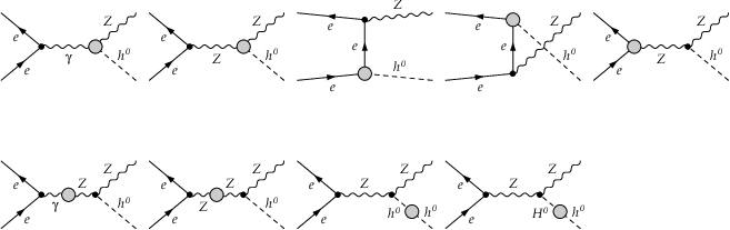
With this renormalization setup in mind, the various contributions to the scattering amplitude of ${}{{}{{{{{\mathrm{{{}{}{{e}^{+}}\mspace{-0.6mu}}}}}}}}}{}{{}{{{{{\mathrm{{{}{}{{e}^{-}}\mspace{-0.6mu}}}}}}}}}\to{}{{}{{{{{\mathrm{{{}{}{{h}^{0}}\mspace{-0.6mu}}}}}}}}}{}{{}{{{{{\mathrm{{{}{}{{Z}}\mspace{-0.6mu}}}}}}}}}^{0}$ at one-loop (Figs. 1-2) can be classified in a meaningful way. First of all, let us note that all of the one-loop diagrams are of course of order $\mathcal{O}(\alpha^{2}_{ew})$. However, some of them include, in addition, enhancement factors sourced by the trilinear Higgs boson couplings $\lambda_{3H}$, see Table II of [32]. In such cases, we shall include these factors when assessing the order of magnitude of the diagram. We are now ready for sorting out the one-loop contributions in different categories:

• •

  Self-energy corrections to the ${}{{}{{{{{\mathrm{{{}{}{{Z}}\mspace{-0.6mu}}}}}}}}}^{0}$ and ${}{{}{{{{{\mathrm{{{}{}{{\gamma}}\mspace{-0.6mu}}}}}}}}}-{}{{}{{{{{\mathrm{{{}{}{{Z}}\mspace{-0.6mu}}}}}}}}}^{0}$ mixing propagators, all of them of order $\mathcal{O}(\alpha^{2}_{ew})$ with no enhancement factors at this order.

• •

  Vertex corrections to the ${}{{}{{{{{\mathrm{{{}{}{{e}^{+}}\mspace{-0.6mu}}}}}}}}}{}{{}{{{{{\mathrm{{{}{}{{e}^{-}}\mspace{-0.6mu}}}}}}}}}{}{{}{{{{{\mathrm{{{}{}{{Z}}\mspace{-0.6mu}}}}}}}}}^{0}$ interaction, which are also of order $\mathcal{O}(\alpha^{2}_{ew})$. It should be noted that we do not include the virtual photonic $\mathcal{O}(\alpha_{em}\,\alpha_{ew})$ effects nor the real bremsstrahlung emission off the ${}{{}{{{{{\mathrm{{{}{}{{e}^{+}}\mspace{-0.6mu}}}}}}}}}/{}{{}{{{{{\mathrm{{{}{}{{e}^{-}}\mspace{-0.6mu}}}}}}}}}$ legs. These pure QED corrections and the weak ones factorize into two subsets which are separately UV finite and gauge-invariant. Moreover, these photonic contributions are fully insensitive, at the order under consideration, to the relevant 3H self-couplings on which we focus. For this kind of processes involving electrically neutral Higgs bosons in the final state, the one-loop QED effects are confined to the initial ${}{{}{{{{{\mathrm{{{}{}{{e}^{+}}\mspace{-0.6mu}}}}}}}}}{}{{}{{{{{\mathrm{{{}{}{{e}^{-}}\mspace{-0.6mu}}}}}}}}}$ vertex. In practice, the net outcome of the accompanying initial state radiation (ISR) is to lower the effective center-of-mass energy available for the annihilation process. All in all, these effects are unessential at this stage to test the presence of the new dynamical features triggered by the 2HDM in the Higgs-strahlung events under analysis.

• •

  Vertex corrections to the ${}{{}{{{{{\mathrm{{{}{}{{e}^{+}}\mspace{-0.6mu}}}}}}}}}{}{{}{{{{{\mathrm{{{}{}{{e}^{-}}\mspace{-0.6mu}}}}}}}}}{}{{}{{{{{\mathrm{{{}{}{{H}}\mspace{-0.6mu}}}}}}}}}$ interaction. Since we have explicitly set $m_{e}=0$ throughout our calculation, the ${}{{}{{{{{\mathrm{{{}{}{{e}^{+}}\mspace{-0.6mu}}}}}}}}}{}{{}{{{{{\mathrm{{{}{}{{e}^{-}}\mspace{-0.6mu}}}}}}}}}{}{{}{{{{{\mathrm{{{}{}{{H}}\mspace{-0.6mu}}}}}}}}}$ tree-level Yukawa coupling is absent and the corresponding one-loop diagrams automatically render a UV finite contribution which is, in any case, very small.

• •

  The loop-induced ${}{{}{{{{{\mathrm{{{}{}{{\gamma}}\mspace{-0.6mu}}}}}}}}}{}{{}{{{{{\mathrm{{{}{}{{Z}}\mspace{-0.6mu}}}}}}}}}^{0}\,{}{{}{{{{{\mathrm{{{}{}{{h}^{0}}\mspace{-0.6mu}}}}}}}}}$ interaction. This one is order $\mathcal{O}(e\,\alpha_{ew}\,\lambda_{3H})$ and therefore includes an enhancement factor $\lambda_{3H}$ . Due to the ${}{{}{{{{{\mathrm{{{}{}{{\gamma}}\mspace{-0.6mu}}}}}}}}}-{}{{}{{{{{\mathrm{{{}{}{{Z}}\mspace{-0.6mu}}}}}}}}}^{0}$ mixing at one-loop, the following counterterm is needed so as to render a UV-finite vertex:

  $\displaystyle\delta\,\mathcal{L}_{{}{{}{{{{{\mathrm{{{}{}{{h}^{0}}\mspace{-0.6mu}}}}}}}}}{}{{}{{{{{\mathrm{{{}{}{{Z}}\mspace{-0.6mu}}}}}}}}}^{0}{}{{}{{{{{\mathrm{{{}{}{{\gamma}}\mspace{-0.6mu}}}}}}}}}}$

  $\displaystyle=$

  $\displaystyle\frac{e\,\sin(\beta-\alpha)\,M_{Z}\,}{2s_{W}c_{W}}\,\delta\,Z_{{}{{}{{{{{\mathrm{{{}{}{{\gamma}}\mspace{-0.6mu}}}}}}}}}{}{{}{{{{{\mathrm{{{}{}{{Z}}\mspace{-0.6mu}}}}}}}}}^{0}}\,g^{\mu\nu}\,{}{{}{{{{{\mathrm{{{}{}{{Z}}\mspace{-0.6mu}}}}}}}}}^{0}_{\mu}\,A_{\nu}\,{}{{}{{{{{\mathrm{{{}{}{{h}^{0}}\mspace{-0.6mu}}}}}}}}}\,.$

  and similarly for the counterterm associated to the effective $\mathcal{L}_{{}{{}{{{{{\mathrm{{{}{}{{H}^{0}}\mspace{-0.6mu}}}}}}}}}{}{{}{{{{{\mathrm{{{}{}{{Z}}\mspace{-0.6mu}}}}}}}}}^{0}{}{{}{{{{{\mathrm{{{}{}{{\gamma}}\mspace{-0.6mu}}}}}}}}}}$ interaction:

  $\displaystyle\delta\,\mathcal{L}_{{}{{}{{{{{\mathrm{{{}{}{{H}^{0}}\mspace{-0.6mu}}}}}}}}}{}{{}{{{{{\mathrm{{{}{}{{Z}}\mspace{-0.6mu}}}}}}}}}^{0}{}{{}{{{{{\mathrm{{{}{}{{\gamma}}\mspace{-0.6mu}}}}}}}}}}$

  $\displaystyle=$

  $\displaystyle\frac{e\,\cos(\beta-\alpha)\,M_{Z}}{2s_{W}c_{W}}\,\delta\,Z_{{}{{}{{{{{\mathrm{{{}{}{{\gamma}}\mspace{-0.6mu}}}}}}}}}{}{{}{{{{{\mathrm{{{}{}{{Z}}\mspace{-0.6mu}}}}}}}}}^{0}}\,g^{\mu\nu}\,{}{{}{{{{{\mathrm{{{}{}{{Z}}\mspace{-0.6mu}}}}}}}}}^{0}_{\mu}\,A_{\nu}\,{}{{}{{{{{\mathrm{{{}{}{{H}^{0}}\mspace{-0.6mu}}}}}}}}}\,,$

• •

  The vertex correction for $h{}{{}{{{{{\mathrm{{{}{}{{Z}}\mspace{-0.6mu}}}}}}}}}^{0}{}{{}{{{{{\mathrm{{{}{}{{Z}}\mspace{-0.6mu}}}}}}}}}^{0}$ encompasses different contributions of order $\mathcal{O}(\alpha^{2}_{ew},\,\alpha_{ew}\,e\,\lambda_{3H})$ (see the sample diagrams in Fig. 3). And, most important, there are, in addition, corrections of $\,\mathcal{O}(\alpha_{ew}\,\lambda^{2}_{3H})$ (in fact, the dominant ones) which are characterized by the highly conspicuous enhancement factor squared $\lambda^{2}_{3H}$. The latter originates from the associated vertex counterterm, most particularly from the Higgs field renormalization constant $Z_{{}{{}{{{{{\mathrm{{{}{}{{h}^{0}}\mspace{-0.6mu}}}}}}}}}}^{1/2}=1+(1/2)\delta\,Z_{{}{{}{{{{{\mathrm{{{}{}{{h}^{0}}\mspace{-0.6mu}}}}}}}}}}$. As we shall discuss in more detail below, $\delta\,Z_{{}{{}{{{{{\mathrm{{{}{}{{h}^{0}}\mspace{-0.6mu}}}}}}}}}}$ is sensitive to the scalar-scalar self-energy and hence it involves products of two triple Higgs self-couplings (see Fig. 4). Of course, an equivalent discussion holds for the complementary channel, ${}{{}{{{{{\mathrm{{{}{}{{H}^{0}}\mspace{-0.6mu}}}}}}}}}\,{}{{}{{{{{\mathrm{{{}{}{{Z}}\mspace{-0.6mu}}}}}}}}}^{0}$.

  The full form of the associated one-loop vertex counterterms ensues from the usual splitting of bare fields and parameters into the renormalized ones and associated counterterms, to wit:

  $$\mathcal{L}\left(g_{0}=g+\delta g,\phi_{0}=Z_{i}^{1/2}\phi\right)\to\mathcal{L}(g,\phi)+\delta\,\mathcal{L}\,.$$

  (8)

  For the ${}{{}{{{{{\mathrm{{{}{}{{h}^{0}}\mspace{-0.6mu}}}}}}}}}{}{{}{{{{{\mathrm{{{}{}{{Z}}\mspace{-0.6mu}}}}}}}}}^{0}{}{{}{{{{{\mathrm{{{}{}{{Z}}\mspace{-0.6mu}}}}}}}}}^{0}$ and ${}{{}{{{{{\mathrm{{{}{}{{H}^{0}}\mspace{-0.6mu}}}}}}}}}{}{{}{{{{{\mathrm{{{}{}{{Z}}\mspace{-0.6mu}}}}}}}}}^{0}{}{{}{{{{{\mathrm{{{}{}{{Z}}\mspace{-0.6mu}}}}}}}}}^{0}$ case one gets respectively:

  	$\displaystyle\hskip-19.91684pt\delta\,\mathcal{L}_{{}{{}{{{{{\mathrm{{{}{}{{h}^{0}}\mspace{-0.6mu}}}}}}}}}{}{{}{{{{{\mathrm{{{}{}{{Z}}\mspace{-0.6mu}}}}}}}}}^{0}{}{{}{{{{{\mathrm{{{}{}{{Z}}\mspace{-0.6mu}}}}}}}}}^{0}}$	$\displaystyle=$	$\displaystyle\frac{e\,\sin\,(\beta-\alpha)\,M_{Z}}{s_{W}\,c_{W}}\,\Bigg[\frac{s_{W}^{2}-c_{W}^{2}}{c_{W}^{2}}\,\frac{\delta s_{W}}{s_{W}}+\sin\beta\cos\beta\,\cot{(\beta-\alpha)}\,\frac{\delta\,\tan\beta}{\tan\beta}$		(9)
  			$\displaystyle+\frac{\delta\,e}{e}+\frac{\delta\,M_{Z}^{2}}{2\,M_{Z}^{2}}+\frac{1}{2}\,\delta\,Z_{{}{{}{{{{{\mathrm{{{}{}{{h}^{0}}\mspace{-0.6mu}}}}}}}}}}+\frac{1}{2}\,\delta\,Z_{{}{{}{{{{{\mathrm{{{}{}{{Z}}\mspace{-0.6mu}}}}}}}}}^{0}}+\frac{1}{2}\,\cot{(\beta-\alpha)}\,\delta Z_{{}{{}{{{{{\mathrm{{{}{}{{H}^{0}}\mspace{-0.6mu}}}}}}}}}{}{{}{{{{{\mathrm{{{}{}{{h}^{0}}\mspace{-0.6mu}}}}}}}}}}\Bigg]\,g^{\mu\nu}\,{}{{}{{{{{\mathrm{{{}{}{{Z}}\mspace{-0.6mu}}}}}}}}}^{0}_{\mu}{}{{}{{{{{\mathrm{{{}{}{{Z}}\mspace{-0.6mu}}}}}}}}}^{0}_{\nu}{}{{}{{{{{\mathrm{{{}{}{{h}^{0}}\mspace{-0.6mu}}}}}}}}}\,,$

  	$\displaystyle\hskip-19.91684pt\delta\,\mathcal{L}_{{}{{}{{{{{\mathrm{{{}{}{{H}^{0}}\mspace{-0.6mu}}}}}}}}}{}{{}{{{{{\mathrm{{{}{}{{Z}}\mspace{-0.6mu}}}}}}}}}^{0}{}{{}{{{{{\mathrm{{{}{}{{Z}}\mspace{-0.6mu}}}}}}}}}^{0}}$	$\displaystyle=$	$\displaystyle\frac{e\,\cos\,(\beta-\alpha)\,M_{Z}}{s_{W}\,c_{W}}\,\Bigg[\frac{s_{W}^{2}-c_{W}^{2}}{c_{W}^{2}}\,\frac{\delta s_{W}}{s_{W}}-\sin\beta\cos\beta\,\tan{(\beta-\alpha)}\,\frac{\delta\,\tan\beta}{\tan\beta}$		(10)
  			$\displaystyle+\frac{\delta\,e}{e}+\frac{\delta\,M_{Z}^{2}}{2\,M_{Z}^{2}}+\frac{1}{2}\,\delta\,Z_{{}{{}{{{{{\mathrm{{{}{}{{H}^{0}}\mspace{-0.6mu}}}}}}}}}}+\frac{1}{2}\,\delta\,Z_{{}{{}{{{{{\mathrm{{{}{}{{Z}}\mspace{-0.6mu}}}}}}}}}^{0}}+\frac{1}{2}\,\tan{(\beta-\alpha)}\,\delta Z_{{}{{}{{{{{\mathrm{{{}{}{{H}^{0}}\mspace{-0.6mu}}}}}}}}}{}{{}{{{{{\mathrm{{{}{}{{h}^{0}}\mspace{-0.6mu}}}}}}}}}}\Bigg]\,g^{\mu\nu}\,{}{{}{{{{{\mathrm{{{}{}{{Z}}\mspace{-0.6mu}}}}}}}}}^{0}_{\mu}{}{{}{{{{{\mathrm{{{}{}{{Z}}\mspace{-0.6mu}}}}}}}}}^{0}_{\nu}{}{{}{{{{{\mathrm{{{}{}{{H}^{0}}\mspace{-0.6mu}}}}}}}}}\,,$

  where we can spot in the structure of these formulae the presence of the above mentioned Higgs field renormalization counterterms $\delta\,Z_{{}{{}{{{{{\mathrm{{{}{}{{h}^{0}}\mspace{-0.6mu}}}}}}}}}}$ and $\delta\,Z_{{}{{}{{{{{\mathrm{{{}{}{{H}^{0}}\mspace{-0.6mu}}}}}}}}}}$. The term $\delta\,Z_{{}{{}{{{{{\mathrm{{{}{}{{h}^{0}}\mspace{-0.6mu}}}}}}}}}{}{{}{{{{{\mathrm{{{}{}{{H}^{0}}\mspace{-0.6mu}}}}}}}}}}$ accounts for the WF mixing ${}{{}{{{{{\mathrm{{{}{}{{h}^{0}}\mspace{-0.6mu}}}}}}}}}\leftrightarrow{}{{}{{{{{\mathrm{{{}{}{{H}^{0}}\mspace{-0.6mu}}}}}}}}}$ emerging from the ${}{{}{{{{{\mathrm{{{}{}{{Z}}\mspace{-0.6mu}}}}}}}}}^{0}{}{{}{{{{{\mathrm{{{}{}{{Z}}\mspace{-0.6mu}}}}}}}}}^{0}{}{{}{{{{{\mathrm{{{}{}{{h}^{0}}\mspace{-0.6mu}}}}}}}}}$ and ${}{{}{{{{{\mathrm{{{}{}{{Z}}\mspace{-0.6mu}}}}}}}}}^{0}{}{{}{{{{{\mathrm{{{}{}{{Z}}\mspace{-0.6mu}}}}}}}}}^{0}{}{{}{{{{{\mathrm{{{}{}{{H}^{0}}\mspace{-0.6mu}}}}}}}}}$ vertices.

• •

  The finite wave-function (WF) correction to the external Higgs fields ${}{{}{{{{{\mathrm{{{}{}{{h}^{0}}\mspace{-0.6mu}}}}}}}}}$ or ${}{{}{{{{{\mathrm{{{}{}{{H}^{0}}\mspace{-0.6mu}}}}}}}}}$ (Fig. 4). These are related to the fact that we have chosen the residue of the ${}{{}{{{{{\mathrm{{{}{}{{A}^{\mspace{-2mu}0}}\mspace{-0.6mu}}}}}}}}}$-propagator at its pole to be one, and therefore there is no more freedom to make the same choice for the other Higgs bosons. This entails a finite WF renormalization correction, see Ref.[32] for details. These finite renormalization effects are of utmost importance in this case, as they trigger leading contributions of order $\mathcal{O}(\alpha_{ew}\,\lambda^{2}_{3H})$. They actually drive the very bulk of the quantum effects (see below for a more detailed discussion).

• •

  Finally, the box-type $\mathcal{O}(\alpha^{2}_{ew})$ diagrams (Figure 2), whose contribution is non-negligible, in particular at large center-of-mass energies – since they are not suppressed as $1/{s}$.

wherein the scalar two-point function is defined as in Ref. [49]:

$\mu$ denoting the ’t Hooft mass unit. In the expression (), $M$ denotes the typical mass scale(s) which appear in these one-loop 2-point functions. Owing to the derivative with respect to the external momentum, the 1-point functions do not contribute to the WF renormalization, and hence the quartic Higgs boson self-couplings are not involved in this calculation. This means that the first line of diagrams in Fig. 4 does not actually contribute. We emphasize that the overall sign for this expression depends on the sign of such 2-point function. Notice that $\Re\,eB_{0}^{\prime}(p^{2},M^{2},M^{2})>0$ for $p^{2}<4M^{2}$, which is the case we wish to focus on for the ${}{{}{{{{{\mathrm{{{}{}{{h}^{0}}\mspace{-0.6mu}}}}}}}}}{}{{}{{{{{\mathrm{{{}{}{{Z}}\mspace{-0.6mu}}}}}}}}}^{0}$ channel, and also for ${}{{}{{{{{\mathrm{{{}{}{{H}^{0}}\mspace{-0.6mu}}}}}}}}}{}{{}{{{{{\mathrm{{{}{}{{Z}}\mspace{-0.6mu}}}}}}}}}^{0}$ (as long as the resonant decay ${}{{}{{{{{\mathrm{{{}{}{{H}^{0}}\mspace{-0.6mu}}}}}}}}}\to{}{{}{{{{{\mathrm{{{}{}{{h}^{0}}\mspace{-0.6mu}}}}}}}}}{}{{}{{{{{\mathrm{{{}{}{{h}^{0}}\mspace{-0.6mu}}}}}}}}}$ is forbidden by kinematics). Therefore, in most of the scenarios of interest, such finite WF corrections carry an overall minus sign. Being proportional to $\lambda_{3H}^{2}$, they become the leading quantum effects in the region where the trilinear couplings are enhanced, and as a result they generate a characteristic pattern of quantum effects in which a systematic suppression of the tree-level cross-section is predicted.

The presence of the large negative corrections induced by the Higgs boson self-energies brings forward a characteristic signature for the production cross-sections of the Higgs-strahlung processes (2). This feature is in marked contradistinction to the situation with the Higgs boson pair production mechanisms(1), where the corresponding corrections are just opposite in sign, i.e. large and positive, see [32]. We shall further comment on these interesting and correlated features in the next section. From the general structure of Eq. (), one may anticipate the typical (maximum) size of the quantum effects on the Higgs-strahlung processes as follows:

$f$ being a dimensionless form factor (basically accounting for the behavior of the $B^{\prime}_{0}$ function). The notation $\braket{\dots}$ stands for the various operations of averaging and integration of the squared matrix elements. Taking into account that unitarity limits let the trilinear couplings reach values as large as $\frac{\lambda_{3H}}{M_{W}}\simeq\frac{|\lambda_{5}|}{e}\simeq 30$, and assuming $M\sim 200\,$ and $f\sim\mathcal{O}(1)$, the above estimate typically predicts a strong depletion of the tree-level signal by $\delta_{r}\simeq-90\%$. This prediction falls in the right ballpark of the exact numerical results that will be reported in the next section, which point to a maximum depletion of $\delta_{r}\sim-60\%$.

Before closing this section, let us recall that the counterterm amplitude $\delta\,{\cal M}^{(1)}_{{}{{}{{{{{\mathrm{{{}{}{{e}^{+}}\mspace{-0.6mu}}}}}}}}}{}{{}{{{{{\mathrm{{{}{}{{e}^{-}}\mspace{-0.6mu}}}}}}}}}\to{}{{}{{{{{\mathrm{{{}{}{{h}^{0}}\mspace{-0.6mu}}}}}}}}}{}{{}{{{{{\mathrm{{{}{}{{Z}}\mspace{-0.6mu}}}}}}}}}^{0}}$ derives from a number of renormalization conditions that determine the renormalized coupling constants and fields in a given renormalization framework. As we have said, in our calculation the renormalization is performed in the conventional on-shell scheme in the Feynman gauge, appropriately extended to include the 2HDM Higgs sector. For the latter, we need in particular a renormalization condition for the parameter $\tan\beta=v_{2}/v_{1}$. We adopt the following [53]:

This condition insures that the ratio ${v_{2}}/{v_{1}}$ is always expressed in terms of the true vacua after the renormalization of the Higgs potential. The corresponding counterterm resulting from $\tan\beta\rightarrow\tan\beta+\delta\tan\beta$ can then be computed explicitly:

This counterterm is involved in Eqs. (9)-(10), and it also determines the WF mixing term $\delta\,Z_{{}{{}{{{{{\mathrm{{{}{}{{h}^{0}}\mspace{-0.6mu}}}}}}}}}{}{{}{{{{{\mathrm{{{}{}{{H}^{0}}\mspace{-0.6mu}}}}}}}}}}$ that appears in these equations, as follows: $\delta\,Z_{{}{{}{{{{{\mathrm{{{}{}{{h}^{0}}\mspace{-0.6mu}}}}}}}}}{}{{}{{{{{\mathrm{{{}{}{{H}^{0}}\mspace{-0.6mu}}}}}}}}}}=\sin{2\alpha}(\delta\tan\beta/\tan\beta)$. We refer the reader once more to the exhaustive presentation of Ref. [32] for the renormalization details.

In this section, we present the numerical analysis of the one-loop computation of the Higgs-strahlung processes (2) within the 2HDM. We shall be concerned basically with the following two quantities: i) the predicted cross-section at the Born-level $\sigma^{(0)}$ and at one loop $\sigma^{(0+1)}$; and ii) the relative size of the one-loop quantum corrections:

We have carried out our analysis with the help of the standard algebraic and numerical tools FeynArts, FormCalc and LoopTools [49].

The different Higgs boson mass sets that shall be used hereafter are quoted in Table 1. Let us highlight that, due to their mass splittings (and also to the fact that $M_{{}{{}{{{{{\mathrm{{{}{}{{h}^{0}}\mspace{-0.6mu}}}}}}}}}}\geq 140$ GeV), Sets C and D can only be realized in a general (non-SUSY) 2HDM framework. Furthermore, in view of the value of the charged Higgs mass, Sets A-C are only suitable for type-I 2HDM, whereas Set D is valid for either type-I and type-II 2HDM’s.

Apart from reflecting a variety of possible situations in the 2HDM parameter space, some of these sets can be mimicked by the Higgs boson mass spectrum in supersymmetric theories. For instance, Sets A and B can be ascribed to characteristic benchmark scenarios of Higgs boson mass spectra within the MSSM; in particular, Set B lies in the class of the so-called maximal mixing scenarios [54], for which $M_{{}{{}{{{{{\mathrm{{{}{}{{h}^{0}}\mspace{-0.6mu}}}}}}}}}}$ takes the highest possible values within the MSSM. The numerical mass values for the MSSM-like sets have been obtained with the aid of the program FeynHiggs by taking the full set of EW corrections at one-loop [50].

We remark that the more massive the Higgs bosons are, the stronger the constraints that unitarity imposes over $|\lambda_{5}|$. The maximum (negative) values are roughly attained for $\lambda_{5}\simeq-9$ (Set A); $\lambda_{5}\simeq-10$ (Sets B and C); and $\lambda_{5}\simeq-8$ (Set D).

Before coming to grips with the analysis of the Higgs-strahlung events in the general 2HDM, it is interesting to briefly reconsider the analogue process in the simpler framework of the SM. In Fig. 5 we display the total (one-loop corrected) cross section (left panel), together with the relative radiative correction $\delta_{r}$ (right panel), as a function of the SM Higgs boson mass $M_{{}{{}{{{{{\mathrm{{{}{}{{H}}\mspace{-0.6mu}}}}}}}}}}$. For completeness, and for illustration purposes, we have also included the scenario corresponding to the last Higgs boson mass segment ruled out by LEP at a center-of-mass energy $\sqrt{s}=200$ GeV (see the leftmost vertical band in that figure). The corresponding production rates for the ILC at $\sqrt{s}=500$ GeV and $\sqrt{s}=1$ TeV are smaller than in the LEP case due to the suppression of the s-channel amplitude by the $Z$-boson propagator at higher energies, see Eq. (5), and the larger mass of the produced Higgs boson. Still, the cross-sections for producing SM Higgs bosons of a few hundred GeV at the startup ILC energy ($\sqrt{s}=500$ GeV) lie at the $40-60\,$ level, which leads roughly to $\sim 25,000$ Higgs events for an expected integrated luminosity of $500$ fb^-1. In turn, the one-loop radiative corrections may be either positive or negative, depending on the center-of-mass energy, and lie generally at the level of a few percent, as can be seen in the right panel of Fig. 5. In this panel, we present the evolution of the correction parameter $\delta_{r}$ defined in Eq. (21), as a function of $M_{{}{{}{{{{{\mathrm{{{}{}{{H}}\mspace{-0.6mu}}}}}}}}}}$. The three peaks (also barely seen in the left panel) are correlated to the production thresholds of ${}{{}{{{{{\mathrm{{{}{}{{W}}\mspace{-0.6mu}}}}}}}}}{{}{{{{{\mathrm{{{}{}{{W}}\mspace{-0.6mu}}}}}}}}}^{-}$, ${}{{}{{{{{\mathrm{{{}{}{{Z}}\mspace{-0.6mu}}}}}}}}}^{0}{}{{}{{{{{\mathrm{{{}{}{{Z}}\mspace{-0.6mu}}}}}}}}}^{0}$ and ${}{{}{{{{{\mathrm{{{}{}{{t}}\mspace{-0.6mu}}}}}}}}}{}{}{{}{{}{{{{{\mathrm{{{}{}{{\overline{t}}_{{\mspace{1mu}}}^{\mspace{1mu}{{\raisebox{-1.65764pt}{{${{{\scriptstyle{{{{{\mathrm{{}}}}}}}}}}$}}}}}}\mspace{-0.6mu}}}}}}}}}}$ pairs.

In Figs. 6-9 we illustrate the fundamental phenomenological features associated to the process ${}{{}{{{{{\mathrm{{{}{}{{e}^{+}}\mspace{-0.6mu}}}}}}}}}{}{{}{{{{{\mathrm{{{}{}{{e}^{-}}\mspace{-0.6mu}}}}}}}}}\to{}{{}{{{{{\mathrm{{{}{}{{h}^{0}}\mspace{-0.6mu}}}}}}}}}{}{{}{{{{{\mathrm{{{}{}{{Z}}\mspace{-0.6mu}}}}}}}}}^{0}$ in the scope of the general 2HDM. Fig. 6 summarizes the pattern of radiative corrections $\delta_{r}$ projected onto the $(\tan\beta,\,\lambda_{5})$ and $(\sin\alpha\,,\tan\beta)$ planes, the former at fixed $\alpha=\beta-\pi/2$ and the latter with $\lambda_{5}=-2$. We remark that for $\alpha=\beta-\pi/2$ the ${}{{}{{{{{\mathrm{{{}{}{{h}^{0}}\mspace{-0.6mu}}}}}}}}}{}{{}{{{{{\mathrm{{{}{}{{Z}}\mspace{-0.6mu}}}}}}}}}^{0}{}{{}{{{{{\mathrm{{{}{}{{Z}}\mspace{-0.6mu}}}}}}}}}^{0}$ tree-level coupling takes on the SM form and therefore is maximal. For definiteness, these plots have been generated for a Higgs boson mass spectrum as in Set B (cf. Table  1), and at the fiducial ILC startup center-of-mass energy, $\sqrt{s}=500\,$. Although the range $\tan\beta\gtrsim 1$ is usually the preferred one from the theoretical point of view, we entertain the possibility that $\tan\beta$ can be slightly below $1$ in order to better assess the behavior around this value. Fig. 6 illustrates that the allowed region in the $(\tan\beta,\,\lambda_{5})$ plane is severely restrained by the theoretical constraints stemming from the perturbative unitarity and vacuum stability. On the one hand, $\lambda_{5}>0$ values are strongly disfavored by the vacuum stability condition; on the other hand, the unitarity constraints tend to disfavor moderate and large values of $\tan\beta$ (specially $\tan\beta$ values significantly larger than $1$) as well as of $\tan\beta\ll 1$. Altogether these constraints set an approximate lower bound of $\lambda_{5}\sim-10$ for $\tan\beta\sim 1$ and a rigid upper bound excluding almost all positive values of $\lambda_{5}$ for any $\tan\beta$. The combined set of constraints builds up a characteristic physical domain, with a valley-shaped area centered at $\tan\beta\sim 1$ that sinks into the $\lambda_{5}<0$ region and becomes narrower with growing $|\lambda_{5}|$.

The fact that the curves of constant $\delta_{r}$ do not depend on $\tan\beta$ (left panel of the Fig. 6) is related to the choice $\alpha=\beta-\pi/2$, which we have made in order to consider the situation where the tree-level cross-section for ${}{{}{{{{{\mathrm{{{}{}{{h}^{0}}\mspace{-0.6mu}}}}}}}}}{}{{}{{{{{\mathrm{{{}{}{{Z}}\mspace{-0.6mu}}}}}}}}}^{0}$ production is maximal. For this choice of the mixing angle $\alpha$, it turns out that no particular enhancement shows up for any value of $\tan\beta$, neither from the 3H self-couplings nor from the Higgs-top quark Yukawa couplings. Indeed, under the condition $\alpha=\beta-\pi/2$, the ${}{{}{{{{{\mathrm{{{}{}{{h}^{0}}\mspace{-0.6mu}}}}}}}}}{}{}{{}{{}{{{{{\mathrm{{{}{}{{\overline{t}}_{{\mspace{1mu}}}^{\mspace{1mu}{{\raisebox{-1.65764pt}{{${{{\scriptstyle{{{{{\mathrm{{}}}}}}}}}}$}}}}}}\mspace{-0.6mu}}}}}}}}}}{}{{}{{{{{\mathrm{{{}{}{{t}}\mspace{-0.6mu}}}}}}}}}$ Yukawa coupling does not depend on $\tan\beta$:

and at the same time the 3H self-couplings which are relevant for this channel become independent of $\tan\beta$; notice, for example, that

The final outcome is that the potential dependence of the computed observables on $\tan\beta$ vanishes as long as we stick to these $\alpha=\beta-\pi/2$ configurations – in which the tree-level coupling ${}{{}{{{{{\mathrm{{{}{}{{h}^{0}}\mspace{-0.6mu}}}}}}}}}{}{{}{{{{{\mathrm{{{}{}{{Z}}\mspace{-0.6mu}}}}}}}}}^{0}{}{{}{{{{{\mathrm{{{}{}{{Z}}\mspace{-0.6mu}}}}}}}}}^{0}$ is maximum and formally equivalent to that of the SM ³³ 3 An equivalent discussion would hold for the ${}{{}{{{{{\mathrm{{{}{}{{H}^{0}}\mspace{-0.6mu}}}}}}}}}{}{{}{{{{{\mathrm{{{}{}{{Z}}\mspace{-0.6mu}}}}}}}}}^{0}$ channel, under the complementary condition $\alpha=\beta$.. As a result, the only feasible mechanism able to significantly enhance the quantum effects in these scenarios is by increasing the value of the $|\lambda_{5}|$ parameter (towards more negative values, so as to be consistent with vacuum stability).

Once we depart from the $\alpha=\beta-\pi/2$ setting, we recover of course the expected dependence of the computed observables with $\tan\beta$ (cf. right panel of Fig. 6), but then the lowest order ${}{{}{{{{{\mathrm{{{}{}{{h}^{0}}\mspace{-0.6mu}}}}}}}}}{}{{}{{{{{\mathrm{{{}{}{{Z}}\mspace{-0.6mu}}}}}}}}}^{0}$ production cross section becomes smaller. For $\tan\beta<1$, radiative corrections are boosted as a result of the enhanced 3H self-couplings, and partially also due to the Higgs-top quark Yukawa couplings. Either way, their overall effect is to suppress the tree-level signal, as such leading corrections are triggered primordially by the finite Higgs boson WF corrections. Another source of enhancement of $\delta_{r}$ appears near the region where $\beta\sim\alpha$. However, this effect is not caused by a real increment of the one-loop cross-section $\sigma^{(0+1)}$, but by a mere suppression of the cross-section at the Born-level, i.e. $\sigma^{(0)}$ in the denominator of Eq. (21), and in this sense it is an uninteresting situation.

In Fig. 7 we explore the evolution of the cross section as a function of the center-of-mass energy. We include, in each plot, the tree-level contribution $\sigma^{(0)}$ and the corresponding loop-corrected value, $\sigma^{(0+1)}$, for different values of $\lambda_{5}$. The right panel tracks the related behavior of the quantum correction $\delta_{r}$ as a function of $\sqrt{s}$, for the same set of $\lambda_{5}$ values. The plots are generated for Set B of Higgs boson masses, at fixed $\tan\beta=1$ and $\alpha=\beta-\pi/2$. The leading-order cross section $\sigma^{(0)}$ curve exhibits the expected behavior with $\sqrt{s}$, as it scales with the $s$-channel ${}{{}{{{{{\mathrm{{{}{}{{Z}}\mspace{-0.6mu}}}}}}}}}^{0}$-boson propagator, namely proportional to $1/(s-M_{Z}^{2})$. A similar pattern is also followed by the full loop corrected cross-section.

The range where the relative one-loop correction $\delta_{r}$ is positive is very reduced and it is confined to a regime where the center-of-mass energy is around the startup value for the ILC ($\sqrt{s}\gtrsim 500$ GeV) and where $\lambda_{5}$ adopts the (small) positive values allowed by the constraints. It should not come as a surprise that this behavior is similar to the SM result found in Fig. 5; indeed, being $\lambda_{5}$ small there can not be significant 2HDM enhancements (not even from $\tan\beta$, which is $1$) with respect to the corresponding SM process. Let us recall that for Set B the maximum value of $\lambda_{5}$ allowed by the vacuum stability bounds is $\lambda_{5}\sim 0.65$. Large negative $\lambda_{5}$ values give rise to significant (negative) quantum effects, and translate into loop-corrected cross sections $\sigma^{(0+1)}$ depleted $40\%$ to $70\%$ with respect to the tree-level predictions in the entire range from $\sqrt{s}=500$ GeV to $\sqrt{s}=3$ TeV. Since the tree-level ${}{{}{{{{{\mathrm{{{}{}{{h}^{0}}\mspace{-0.6mu}}}}}}}}}{}{{}{{{{{\mathrm{{{}{}{{Z}}\mspace{-0.6mu}}}}}}}}}^{0}{}{{}{{{{{\mathrm{{{}{}{{Z}}\mspace{-0.6mu}}}}}}}}}^{0}$ coupling is equivalent to the SM coupling ${}{{}{{{{{\mathrm{{{}{}{{H}}\mspace{-0.6mu}}}}}}}}}{}{{}{{{{{\mathrm{{{}{}{{Z}}\mspace{-0.6mu}}}}}}}}}^{0}{}{{}{{{{{\mathrm{{{}{}{{Z}}\mspace{-0.6mu}}}}}}}}}^{0}$ for $\alpha=\beta-\pi/2$, the right panel of Fig. 7 also illustrates the departure of the 2HDM loop-corrected cross section with respect to the tree-level SM cross-section, namely $(\sigma^{(0+1)}_{2HDM}-\sigma_{SM}^{(0)})/\sigma_{SM}^{(0)}$.

The behavior of $\sigma({}{{}{{{{{\mathrm{{{}{}{{e}^{+}}\mspace{-0.6mu}}}}}}}}}{}{{}{{{{{\mathrm{{{}{}{{e}^{-}}\mspace{-0.6mu}}}}}}}}}\to{}{{}{{{{{\mathrm{{{}{}{{h}^{0}}\mspace{-0.6mu}}}}}}}}}{}{{}{{{{{\mathrm{{{}{}{{Z}}\mspace{-0.6mu}}}}}}}}}^{0})$ as a function of the Higgs boson mass $M_{{}{{}{{{{{\mathrm{{{}{}{{h}^{0}}\mspace{-0.6mu}}}}}}}}}}$ is presented in Fig. 8. This figure is the 2HDM counterpart of Fig. 5 corresponding to the SM case. We superimpose the tree-level and the loop-corrected cross-sections for the Set B of Higgs boson masses, by setting $\tan\beta=1$, $\alpha=\beta-\pi/2$ and using three different values of $\lambda_{5}$. The center-of-mass energy is settled at the fiducial value $\sqrt{s}=500$ GeV. Obviously, the raise of the Higgs boson mass $M_{{}{{}{{{{{\mathrm{{{}{}{{h}^{0}}\mspace{-0.6mu}}}}}}}}}}$ implies a reduction of the available phase space, so that the cross-section falls down. In the left panel of Fig. 8, both the tree-level and the loop-corrected cross-sections decrease monotonically with the growing of $M_{{}{{}{{{{{\mathrm{{{}{}{{h}^{0}}\mspace{-0.6mu}}}}}}}}}}$. The ${}{{}{{{{{\mathrm{{{}{}{{Z}}\mspace{-0.6mu}}}}}}}}}^{0}{}{{}{{{{{\mathrm{{{}{}{{Z}}\mspace{-0.6mu}}}}}}}}}^{0}$ and ${}{{}{{{{{\mathrm{{{}{}{{W}}\mspace{-0.6mu}}}}}}}}}^{+}{}{{}{{{{{\mathrm{{{}{}{{W}}\mspace{-0.6mu}}}}}}}}}^{-}$ thresholds are also barely visible therein. In the right panel of the same figure we observe a steady increase of the negative value of the correction for heavier Higgs boson mass, whereas the case with positive correction remains almost stable.

Finally, in Fig. 9 we display the tree-level contribution and the total (one-loop corrected) cross section (left panel), together with the relative radiative correction $\delta_{r}$ (right panel), as a function of the parameter $\lambda_{5}$. These plots have been generated in the same benchmark conditions as in Fig. 8 and using a fiducial ILC start-up center-of-mass energy $\sqrt{s}=500$ GeV. Let us remember that the red shaded area on the right hand side of that figure (specifically for $\lambda_{5}\gtrsim 2.4$) stands for the region excluded by the vacuum stability bounds, whereas the light gray shaded area on the left ($\lambda_{5}\lesssim-10.5$) signals the domain excluded by the perturbative unitarity bounds. The cross section is seen to follow the expected behavior, which we have derived from the estimate of the leading effect – cf. Eq.  () – in combination with the structure of the trilinear coupling (23), namely a negative quadratic dependence of the scattering amplitude, which transates into $\sigma({}{{}{{{{{\mathrm{{{}{}{{e}^{+}}\mspace{-0.6mu}}}}}}}}}{}{{}{{{{{\mathrm{{{}{}{{e}^{-}}\mspace{-0.6mu}}}}}}}}}\to{}{{}{{{{{\mathrm{{{}{}{{h}^{0}}\mspace{-0.6mu}}}}}}}}}{}{{}{{{{{\mathrm{{{}{}{{Z}}\mspace{-0.6mu}}}}}}}}}^{0})\sim(a-b\lambda^{2}_{5})^{2}$, emerging ultimately from the finite WF corrections to the external Higgs boson leg (notice the inclusion of the leading quartic corrections). For moderate negative $\lambda_{5}$, the relative size of the one-loop quantum corrections can reach up to $\sim-50\%$. Positive $\delta_{r}$, however, can only take place for $\lambda_{5}$ close to zero.

A rather comprehensive survey of the predicted cross-sections for different values of the tree-level coupling and different Higgs mass setups is presented in Table 2. We display the results for the one-loop corrected cross-sections (in fb), together with the relative radiative corrections (cf. Eq. (21)), for both neutral Higgs-strahlung channels ${}{{}{{{{{\mathrm{{{}{}{{h}^{0}}\mspace{-0.6mu}}}}}}}}}{}{{}{{{{{\mathrm{{{}{}{{Z}}\mspace{-0.6mu}}}}}}}}}^{0}$ and ${}{{}{{{{{\mathrm{{{}{}{{H}^{0}}\mspace{-0.6mu}}}}}}}}}{}{{}{{{{{\mathrm{{{}{}{{Z}}\mspace{-0.6mu}}}}}}}}}^{0}$. Once more, we set $\sqrt{s}=500\,$; and we work at $\tan\beta=1$ and maximum allowed $|\lambda_{5}|$, since we are mostly interested in spotlighting the imprints of the 3H self-couplings in the quantum effects associated to the Higgs-strahlung mechanism. Let us also recall in passing that $\alpha=\beta-\pi/2$ maximizes the tree-level ${}{{}{{{{{\mathrm{{{}{}{{h}^{0}}\mspace{-0.6mu}}}}}}}}}{}{{}{{{{{\mathrm{{{}{}{{Z}}\mspace{-0.6mu}}}}}}}}}^{0}{}{{}{{{{{\mathrm{{{}{}{{Z}}\mspace{-0.6mu}}}}}}}}}^{0}$ coupling, whilst ${}{{}{{{{{\mathrm{{{}{}{{H}^{0}}\mspace{-0.6mu}}}}}}}}}{}{{}{{{{{\mathrm{{{}{}{{Z}}\mspace{-0.6mu}}}}}}}}}^{0}{}{{}{{{{{\mathrm{{{}{}{{Z}}\mspace{-0.6mu}}}}}}}}}^{0}$ is optimal in the complementary regime, $\alpha=\beta$. From the table we may read out that radiative corrections in these regimes are certainly large, regardless of the details of the chosen mass spectrum, the tree-level coupling and the actual channel under consideration. In a nutshell: the characteristic signature of the enhanced 3H self-couplings in the pattern of quantum effects on the Higgs-strahlung processes is rather universal and manifests in the form of a substantial depletion of the tree-level signal (typically in the range of $\delta_{r}\sim-20/-60\,\%$). Fortunately, even under such a dramatic suppression the final loop-corrected cross sections stay at the level of a few tens of fb – thereby amounting to a non-negligible yield of $\sim 10^{3}-10^{4}$ events per $500\,\invfb$.

A note of caution should be given at this point in regard to some particular configurations of the ${}{{}{{{{{\mathrm{{{}{}{{H}^{0}}\mspace{-0.6mu}}}}}}}}}{}{{}{{{{{\mathrm{{{}{}{{Z}}\mspace{-0.6mu}}}}}}}}}^{0}$ channel. It turns out that certain choices of Higgs boson masses (e.g. for MSSM-like mass splittings) may lie close, or simply beyond, the kinematical threshold for the decay process ${}{{}{{{{{\mathrm{{{}{}{{H}^{0}}\mspace{-0.6mu}}}}}}}}}\to{}{{}{{{{{\mathrm{{{}{}{{h}^{0}}\mspace{-0.6mu}}}}}}}}}{}{{}{{{{{\mathrm{{{}{}{{h}^{0}}\mspace{-0.6mu}}}}}}}}}$; that is to say, $M_{{}{{}{{{{{\mathrm{{{}{}{{H}^{0}}\mspace{-0.6mu}}}}}}}}}}\simeq 2\,M_{{}{{}{{{{{\mathrm{{{}{}{{h}^{0}}\mspace{-0.6mu}}}}}}}}}}$. If we then consider a regime wherein $\alpha=\beta$ and sizable $|\lambda_{5}|$, then the ${}{{}{{{{{\mathrm{{{}{}{{H}^{0}}\mspace{-0.6mu}}}}}}}}}$  WF-correction undergoes a remarkable boost, which results from the combination of two independent sources of enhancement, namely i) the actual strength of the ${}{{}{{{{{\mathrm{{{}{}{{H}^{0}}\mspace{-0.6mu}}}}}}}}}{}{{}{{{{{\mathrm{{{}{}{{h}^{0}}\mspace{-0.6mu}}}}}}}}}{}{{}{{{{{\mathrm{{{}{}{{h}^{0}}\mspace{-0.6mu}}}}}}}}}$ coupling – which is maximally enlarged in this regime; and ii) the kinematical enhancement due to the vicinity of the ${}{{}{{{{{\mathrm{{{}{}{{H}^{0}}\mspace{-0.6mu}}}}}}}}}\to{}{{}{{{{{\mathrm{{{}{}{{h}^{0}}\mspace{-0.6mu}}}}}}}}}{}{{}{{{{{\mathrm{{{}{}{{h}^{0}}\mspace{-0.6mu}}}}}}}}}$ threshold, which is reflected as a sharp peak in $\delta\,Z_{{}{{}{{{{{\mathrm{{{}{}{{H}^{0}}\mspace{-0.6mu}}}}}}}}}}\sim B_{0}^{\prime}(M^{2}_{{}{{}{{{{{\mathrm{{{}{}{{H}^{0}}\mspace{-0.6mu}}}}}}}}}},M^{2}_{{}{{}{{{{{\mathrm{{{}{}{{h}^{0}}\mspace{-0.6mu}}}}}}}}}},M^{2}_{{}{{}{{{{{\mathrm{{{}{}{{h}^{0}}\mspace{-0.6mu}}}}}}}}}})$. However, these ${}{{}{{{{{\mathrm{{{}{}{{H}^{0}}\mspace{-0.6mu}}}}}}}}}$ WF-corrections become so large that the perturbative formula () is no longer valid and we have to keep the original (unexpanded) expression $\hat{Z}^{1/2}_{{}{{}{{{{{\mathrm{{{}{}{{H}^{0}}\mspace{-0.6mu}}}}}}}}}}=\left[1+{\Re e\hat{\Sigma}_{{}{{}{{{{{\mathrm{{{}{}{{H}^{0}}\mspace{-0.6mu}}}}}}}}}}^{\prime}(M^{2}_{{}{{}{{{{{\mathrm{{{}{}{{H}^{0}}\mspace{-0.6mu}}}}}}}}}})}\right]^{-1/2}$. Out of such corner in the parameter space, the higher-order effects involved in the above resummed form of the WF-corrections become harmless and totally inconspicuous and can be safely discarded. If, alternatively, we were considering a mass setup such that $M_{{}{{}{{{{{\mathrm{{{}{}{{H}^{0}}\mspace{-0.6mu}}}}}}}}}}>2M_{{}{{}{{{{{\mathrm{{{}{}{{h}^{0}}\mspace{-0.6mu}}}}}}}}}}$, then the decay ${}{{}{{{{{\mathrm{{{}{}{{H}^{0}}\mspace{-0.6mu}}}}}}}}}\to{}{{}{{{{{\mathrm{{{}{}{{h}^{0}}\mspace{-0.6mu}}}}}}}}}{}{{}{{{{{\mathrm{{{}{}{{h}^{0}}\mspace{-0.6mu}}}}}}}}}$ would be open and, in the scenario of maximum ${}{{}{{{{{\mathrm{{{}{}{{H}^{0}}\mspace{-0.6mu}}}}}}}}}{}{{}{{{{{\mathrm{{{}{}{{h}^{0}}\mspace{-0.6mu}}}}}}}}}{}{{}{{{{{\mathrm{{{}{}{{h}^{0}}\mspace{-0.6mu}}}}}}}}}$ coupling, it would furnish a very large width for ${}{{}{{{{{\mathrm{{{}{}{{H}^{0}}\mspace{-0.6mu}}}}}}}}}$. In this particular setup, the process would effectively boil down to the double Higgs-strahlung channels ${}{{}{{{{{\mathrm{{{}{}{{e}^{+}}\mspace{-0.6mu}}}}}}}}}{}{{}{{{{{\mathrm{{{}{}{{e}^{-}}\mspace{-0.6mu}}}}}}}}}\to{}{{}{{{{{\mathrm{{{}{}{{H}^{0}}\mspace{-0.6mu}}}}}}}}}{}{{}{{{{{\mathrm{{{}{}{{Z}}\mspace{-0.6mu}}}}}}}}}^{0}\to{}{{}{{{{{\mathrm{{{}{}{{h}^{0}}\mspace{-0.6mu}}}}}}}}}{}{{}{{{{{\mathrm{{{}{}{{h}^{0}}\mspace{-0.6mu}}}}}}}}}{}{{}{{{{{\mathrm{{{}{}{{Z}}\mspace{-0.6mu}}}}}}}}}^{0}$ previously explored in the literature [22].

References

- [1] P.W. Higgs, Phys. Lett. 12 (1964) 32; Phys. Rev. Lett. 13 (1964) 508; F. Englert and R. Brout, Phys. Rev. Lett. 13 (1964) 321. G.S Guralnik, C.R. Hagen and T. W. B. Kibble, Phys. Rev. Lett. 13 (1964) 585.
- [2] H.P Nilles, Phys. Rep 110 (1984) 1; H.E. Haber and G.L. Kane, Phys. Rep 117 (1985) 75; S.Ferrara, ed., Supersymmetry, vol.1-2 North Holland/World Scientific, Singapore, 1987.
- [3] J. A. Coarasa, D. García, J. Guasch, R. A. Jiménez, J. Solà, Eur. Phys. J. C2, 373 (1998), arXiv:hep-ph/9607485; Phys. Lett. B425 (1998) 329, arXiv:hep-ph/9711472.
- [4] R. A. Jiménez, J. Solà, Phys. Lett. B389 (1996) 53; J.A. Coarasa, R. A. Jiménez, J. Solà, Phys. Lett. B389 (1996) 312; J. Guasch, R. A. Jiménez, J. Solà, Phys. Lett. B360 (1995) 47; D. García, R. A. Jiménez, J. Solà, W. Hollik, Nucl. Phys. B427 (1994) 53.
- [5] J. Guasch, W. Hollik, J. Solà, JHEP 0210 (2002) 040; Phys. Lett. B510 (2001) 211; Phys. Lett. B437 (1998) 88.
- [6] M. S. Carena, D. García, U. Nierste, C.E.M. Wagner Nucl. Phys. B577 (2000) 88; Phys. Lett. B499 (2001) 141.
- [7] A. Belyaev, D. García, J. Guasch, J. Solà, Phys. Rev. D65 (2002) 031701; JHEP 0206 (2002) 059.
- [8] M. S. Carena, H. E. Haber, Prog. Part. Nucl. Phys. 50 (2003) 63, arXiv:hep-ph/0208209.
- [9] A. Djouadi, Phys. Rep 459 (2008) 1, arXiv:hep-ph/0503172; Phys. Rep 457 (2008) 1, arXiv:hep-ph/0503173.
- [10] S. Heinemeyer, Acta Phys. Polon. B39 (2008) 2673, arXiv:0807.2514 [hep-ph]; Higgs and Electroweak Physics, arXiv:0912.0361 [hep-ph].
- [11] J.F. Gunion, H.E. Haber, G.L. Kane and S. Dawson, The Higgs hunter’s guide, Addison-Wesley, Menlo-Park, 1990.
- [12] J.A. Coarasa, J. Guasch, J. Solà and W. Hollik, Phys. Lett. B442 (1998) 326, arXiv:hep-ph/9808278.
- [13] S. Béjar, J. Guasch, J. Solà, Nucl. Phys. B600 (2001) 21, arXiv:hep-ph/0011091; Nucl. Phys. B675 (2003) 270, arXiv:hep-ph/0307144.
- [14] J. Guasch, J. Solà, Nucl. Phys. B562 (1999) 3, arXiv:hep-ph/9906268.
- [15] S. Béjar, J. Guasch, D. López-Val, J. Solà, Phys. Lett. B668 (2008) 364, arXiv:0805.0973 [hep-ph]; D. López-Val, J. Guasch, J. Solà, JHEP 0712 (2007) 054, arXiv:0710.0587 [hep-ph]; J. Guasch, W. Hollik, S. Peñaranda, J. Solà, Nucl. Phys. Proc. Suppl. 157 (2006) 152, arXiv:hep-ph/0601218; G. Eilam, M. Frank, I. Turan, Phys. Rev. D74 (2006) 035012, arXiv:hep-ph/0601253.
- [16] P. Draper, T. Liu, C.E.M. Wagner, Phys. Rev. D80 (2009) 035025, arXiv:0905.4721 [hep-ph].
- [17] A. Arhrib, R. Benbrik, C-H. Chen, R. Guedes, R. Santos, JHEP 0908 (2009) 035, arXiv:0906.0387 [hep-ph].
- [18] G. Weiglein et al., Phys. Rep 426 (2006) 47, arXiv:hep-ph/0410364.
- [19] For the ILC see http://www.linearcollider.org/cms/; for CLIC, see http://clic-study.web.cern.ch/clic-study/ .
- [20] A. Djouadi, W. Kilian, M. Mühlleitner and P.M. Zerwas, Eur. Phys. J C10 (1999) 27, hep-ph/9903229; M. Mühlleitner, arXiv:hep-ph/0008127.
- [21] G. Ferrera, J. Guasch, D. López-Val and J. Solà, Phys. Lett. B659 (2008) 297, arXiv:0707.3162 [hep-ph]; PoS RADCOR2007, 043 (2007), arXiv:0801.3907 [hep-ph].
- [22] A. Arhrib, R. Benbrik and C.-W. Chiang, Phys. Rev. D77 (2008) 115013, arXiv:0802.0319 [hep-ph]; A. Arhrib, R. Benbrik, and C.-W. Chiang, AIP Conf. Proc. 1006, 112 (2008).
- [23] R. N. Hodgkinson, D López-Val and J. Solà, Phys. Lett. B673 (2009) 47, arXiv:0901.2257 [hep-ph].
- [24] M. Krawczyk, presented at the Int. Workshop on Linear Colliders (LCWS 2002) and references therein, arXiv:hep-ph/0307314.
- [25] N. Bernal, D. López-Val and J. Solà, Phys. Lett. B677 (2009) 38, arXiv:0903.4978 [hep-ph]; P. Posch, arXiv:1001.1759.
- [26] F. Cornet and W. Hollik, Phys. Lett. B669 (2008) 58, arXiv:0808.0719 [hep-ph]; E. Asakawa, D. Harada, S. Kanemura, Y. Okada and K. Tsumura, Phys. Lett. B672 (2009) 354,arXiv:0809.0094 [hep-ph]; A. Arhrib, R. Benbrik, C.-H. Chen, and R. Santos, Phys. Rev. D80 (2009) 015010 arXiv:0902.2458 [hep-ph].
- [27] P. Chankowski, S. Pokorski and J. Rosiek, Nucl. Phys. B423 (1994) 437, arXiv:0902.2458 [hep-ph]; P. H. Chankowski and S. Pokorski, Phys. Lett. B356 (1995) 307, arXiv:hep-ph/9505308.
- [28] V. Driesen and W. Hollik, Zeitsch. f. Physik C68 (1995) 485, arXiv:hep-ph/9504335; V. Driesen, W. Hollik and J. Rosiek, Zeitsch. f. Physik C71 (1996) 259, arXiv:hep-ph/9512441; V. Driesen, W. Hollik and J. Rosiek, arXiv:hep-ph/9605437.
- [29] S. Heinemeyer, W. Hollik, J. Rosiek and G. Weiglein, Eur. Phys. J C19 (2001) 535, arXiv:hep-ph/0102081.
- [30] J. L. Feng and T. Moroi, Phys. Rev. D56 (1997) 5962, arXiv:hep-ph/9612333; E. Coniavitis and A. Ferrari, Phys. Rev. D75 (2007) 015004.
- [31] A. Arhrib and G. Moultaka, Nucl. Phys. B558 (1999) 3, arXiv:hep-ph/9808317; A. Kraft, PhD thesis, Universität Karlsruhe, 1999; J. Guasch, W. Hollik and A. Kraft, Nucl. Phys. B558 (1999) 3; arXiv:hep-ph/9911452.
- [32] D. López-Val and J. Solà, Phys. Rev. D81 (2010) 033003, arXiv:0908.2898 [hep-ph]. For a summarized presentation, see D. López-Val and J. Solà, PoS (RADCOR2009) 045, arXiv:1001.0473 [hep-ph].
- [33] J.F. Gunion, H.E. Haber and J. Wudka, Phys. Rev. D43 (1991) 904.
- [34] A. Djouadi, H.E. Haber and P.M. Zerwas, Phys. Lett. B375 (1996) 203, arXiv:hep-ph/9602234; A. Djouadi, V. Driesen, W. Hollik and J. Rosiek, Nucl. Phys. B491 (1997) 68, arXiv:hep-ph/9609420;
- [35] J.D. Bjorken, in: proc. of the 1976 SLAC Summer Institute on Particle Physics, ed. M. Zipf (SLAC Report No. 198, 1976) p. 22; D.R.T. Jones and S.T. Petcov, Phys. Lett. B84 (1979) 440.
- [36] The Particle Data Group (C. Amsler et al.) , Phys. Lett. B667 (2008) 1.
- [37] E. Gross, G. Wolf and B. A. Kniehl, Zeitsch. f. Physik C63 (1996) 417; G. Altarelli, T. Sjöstrand and F. Zwirner (eds.), Physics at LEP2 in CERN 96-01 (1996); Erratum ibid. C66 (1995) 321
- [38] A. Djouadi, J. Kalinowski and P. Zerwas, Zeitsch. f. Physik C57 (1993) 569, arXiv:hep-ph/9603368; P.H. Chankowski, S. Pokorski and J. Rosiek, Nucl. Phys. B423 (1994) 497; V. Driesen and W. Hollik, Zeitsch. f. Physik C68 (1995) 485; V. Driesen, W. Hollik and J. Rosiek, Zeitsch. f. Physik C71 (1996) 259; A. Djouadi, J. Kalinowski, P. Ohmann and P. Zerwas, Zeitsch. f. Physik C74 (1997) 93, arXiv:hep-ph/9605339.
- [39] K. E. Williams, G. Weiglein, in preparation.
- [40] M. Frank , T. Hahn, S. Heinemeyer, W. Hollik, H. Rzehak, G. Weiglein, JHEP 0702 (2007) 047, arXiv: hep-ph/0611326.
- [41] M.B. Einhorn, D. R. T. Jones and M. J. G. Veltman, Nucl. Phys. B123 (1977) 89.
- [42] M. Misiak and M. Steinhauser, Nucl. Phys. B764 (2007) 62, arXiv:hep-ph/0609241; M. Misiak et al., Phys. Rev. Lett. 98 (2007) 022002, arXiv:hep-ph/0609232.
- [43] V. D. Barger, J. L. Hewett, R. J. N. Phillips, Phys. Rev. D41 (1990) 3421; A. G. Akeroyd, Phys. Lett. B368 (1996) 89.
- [44] S. Kanemura, T. Kubota and E. Takasugi, Phys. Lett. B313 (1993) 155, arXiv:hep-ph/9303263; A.Arhrib, arXiv:hep-ph/0012353; A. G. Akeroyd, A. Arhrib and E.-M. Naimi, Phys. Lett. B490 (2000) 119, arXiv:hep-ph/0006035.
- [45] M. Sher, Phys. Rep 179 (1989) 273; S. Nie and M. Sher, Phys. Lett. B449 (1999) 89, arXiv:hep-ph/9811234.
- [46] D. Kominis and R. S. Chivukula, Phys. Lett. B304 (1993) 152, arXiv:hep-ph/9301222; S. Kanemura, T. Kasai and Y. Okada, Phys. Lett. B471 (1999) 182, arXiv:hep-ph/9903289.
- [47] K. Aoki, Z. Hioki, M. Konuma, R. Kawabe and T. Muta, Prog. Theor. Phys. Suppl. G73 (1982) 1; M. Bohm, H. Spiesberger and W. Hollik, Fortsch. Phys. G34 (1986) 87; A. Sirlin, Phys. Rev. D22 (1980) 971; W. Hollik, in: Precision tests of the Standard Electroweak Model, Ed. P. Langacker, Advanced Series on Directions in High Energy Physics - Vol. 14 (World Scientific, 1995); A. Denner, Fortsch. Phys. G41 (1993) 307.
- [48] S. Heinemeyer, W. Hollik, and G. Weiglein, Phys. Rep 425 (2006) 265, eprint arXiv:hep-ph/0412214.
- [49] T. Hahn, FeynArts 3.2, FormCalc and LoopTools user’s guides, available from http://www.feynarts.de; T. Hahn, Comput. Phys. Commun. 168 (2005) 78.
- [50] S. Heinemeyer, W. Hollik and G. Weiglein, Comput. Phys. Comm. 124 (2000) 76; S. Heinemeyer, T. Hahn, http://www.feynhiggs.de/.
- [51] F. Yuasa et al, Prog. Theor. Phys. Suppl. 138 (2000) 18 ; J. Fujimoto et al. Comput. Phys. Comm. 153 (2003)106; J. Fujimoto et al, Phys. Rev. D75 (2007) 113002.
- [52] N. Baro, F. Boudjema, and A. Semenov, Phys. Rev. D78 (2008) 115003, arXiv:0807.4668 [hep-ph]; N. Baro, F. Boudjema, Phys. Rev. D80 (2009) 076010, eprint arXiv:0906.1665 [hep-ph].
- [53] A. Dabelstein, Zeitsch. f. Physik C67 (1995) 495, eprint arXiv:hep-ph/9409375; Nucl. Phys. B456 (1995) 25, eprint arXiv:hep-ph/9503443.
- [54] M. Carena, S. Heinemeyer, C. E. M. Wagner and G. Weiglein, Eur. Phys. J C26 (2003) 601, arXiv:hep-ph/0202167.
- [55] CDF and D0 Collaborations, arXiv:0903.4001 [hep-ex]; N. Krumnack, arXiv:0910.3353 [hep-ex].
- [56] J.A. Grifols, A. Méndez, Phys. Rev. D22 (1980) 1725.
- [57] J.A. Grifols, J. Solà, Phys. Rev. D23 (1981) 95.
- [58] A. Arhrib, M. Capdequi Peyranere, W. Hollik, G. Moultaka, Nucl. Phys. B581 (2000) 34, arXiv:hep-ph/9912527.
- [59] O. Brein and T. Hahn, Eur. Phys. J C52 (2007) 397, arXiv:hep-ph/0610079.
- [60] F. Mahmoudi and O. Stal, Phys. Rev. D81 (2010) 035016, arXiv:0907.1791.