Localizing Gauge Fields on a Topological Abelian String and the Coulomb Law.
Abstract
The confinement of electromagnetic field is studied in axial symmetrical, warped, 6D World Brane, using a recently proposed topological abelian string vortex solution as background. It was found, that the massless gauge field fluctuations follow 4D Maxwell equations in the Lorenz gauge. The massless zero mode is localized when the thickness of the string-vortex is less than 5/4 there are not others localized massless modes. There is also an infinite of non localized massive Fourier modes, that follow 4 dimensional Proca equations with a continuous spectrum. To compute the corrections to the Coulomb potential, a radial cutoff was introduced, in order to achieve a discrete mass spectrum. As main result, a correction was found for the 4D effective Coulomb law, the result is in correspondence with the observed behavior of the Coulomb potential at nowadays measurable distances.
PACS numbers: 04.20.-q, 11.27.+d, 04.50.+h
I Introduction
In the brane world view, the universe is considered a 3-brane contained in some topological defect. This 3-brane is embedded in non compact, large, extra dimensional spacetime with finite volume [1] usually with warping metric [2] in the directions of the additional dimensions. Most of the research had been done [3] on domain walls in 5 dimensions, due to the fact that this is the simplest kind of topological defect and exact solutions are available for both the metric and scalar fields. Important advances had been made on domain wall’s brane world, as possible explanation to the hierarchy problem [2], localization of gravity [5], and the confinement of some fundamental fields [4] as chiral fermions [7], but there are still several unsolved problems as the localization of gauge fields [8][4], stability under casimir energy or quantum fluctuations [6] and the lack of a complete supersymmetric version.
Its is widely known that in 5 dimensional brane worlds, the gauge and spinor fields can scape from the 3 brane universe into the bulk. Yukawa coupling gives a natural way of localize fermionic fields on topological defects [7] but the confinement of spin 1 fields remains as an open problem. Some mechanisms as DS [8] and DGS [9] of quasi localization has been proposed. These mechanism seem to unnaturally force, or increase the effect of the ”wall” over the volumetric ”bulk” terms. To do that, they introduce two different coupling constant for the electromagnetic field and very strict restrictions on the fields and parameters. Some recent calculations indicate very strict bounds on the wall thickness of many orders of magnitude thinner than the Planck scale [10] to achieve a 4 dimensional behavior. The loss of electromagnetic radiation at low frequency and the non preservation of charge are also drawbacks related to the confinement of gauge fields in domain wall brane worlds. Although this drawbacks can be controlled in several ways, they are also unwanted features for a theory modeling the universe.
Some years ago, brane worlds had been proposed over more complicated topological defect than domain walls. For example world brane had been proposed for the 6 dimensional vortex [11][12] and 7 dimensional monopole [13][14]. The confinement of spin 1 gauge fields [15] seems to be possible to achieve in string-vortices in 6 dimensions: it has been found that electromagnetic gauge field fluctuations has a localized zero mode [15][16], however the graviphoton zero modes (spin 1 fluctuations of the metric) are not normalizable due to its behavior either at infinity or very near to the string-vortex [17][18]. These works are based on numerical or asymptotical approximations, because there are not known general analytic solutions for curved 6D string-vortices and very few exact solutions had been reported [19][20]. Moreover, almost nothing is known about the non zero modes and its influence on the propagators, potentials and interactions.
Recently, new Randall Sundrum scenarios in 6 dimensional curved space time based on exact topological solutions to the abelian higgs model [20] had been reported. These solutions correspond to different Einstein Maxwell field vacua, with scalar kink solitons and auto-interaction potential, that are in fact, electromagnetic uncharged string-vortices with non trivial winding number. These topological abelian strings exhibits a localized spin 2 zero mode, that gives rise to the newtonian gravity, while the rest of the modes gives account of a correction to the potential [11]. Is the purpose of these paper to study the confinement of spin 1 gauge field, on a background of a 6 dimensional topological abelian string vortex, in order to establish the localization or not, of all the photon’s fourier modes and calculate the corrections to the Coulomb law.
The organization of the paper is as follows: section II explains the model: the topological abelian string vortex. Section III reviews the confinement of the zero mode of linearized gravity and the non confinement of the other modes. In section IV, the gauge fixing conditions and the decoupling from the graviphotons and graviscalars field are discussed and the 4D Maxwell equations recovered in a perturbative approach using the topological abelian string as background. In section V, the gauge field equations are expanded in Fourier modes. A localized, normalizable, solution to the massless zero mode is obtained numerically in the thin string approximation: it is shown that there are not other localized massless modes. In section VI the massive modes are studied, a regularization is proposed based on the introduction of a radial cutoff and the corrections to the Coulomb law calculated. It is the main result of this paper a correction to the Coulomb potential. In section VII the range of validity of this corrections and its adjustment to known experimental bounds is discussed, finally some conclusions and remarks are presented.
II A Topological Einstein Abelian String-Vortex Solution.
We start from the 6 dimensional action
| (1) |
where the first integral is the 6D Einstein Hilbert action, with a bulk cosmological constant and is the covariant derivative.
In what follows we will set where is the 6D Planck mass and we will follow the notation in [12]11 1 and uppercase Latin indices run over 4+2 dim. and Greek indices over 4 dim. middle alphabet Latin indices run in 3 dim and firsts alphabet Latin indices run over 2 dim Bold was used for mass.
Here we will look for a geometry 2+3+1 composed by a 3-brane that contains the 3+1 physical universe and 2 extra dimensions, where we can choose coordinates and the metric is given by:
| (2) |
with . In this context and are the coordinates of the extra dimension, acts as a radial factor and is a warp factor, rapidly diminishing when moving away from a 4 dimensional 3-brane located at .
Assuming that the scalar and gauge fields in (1) depends on the extra coordinates as in the Nielsen Olesen ansatz [21][11]
| (3) | |||||
| (4) | |||||
| (5) | |||||
| (6) |
where the is dimensional factor with units . Performing variations in the action (1) we get the curved version of Nielsen Olesen vortex equations [12]:
| (7) | |||||
| (8) |
where
String-vortex solutions are classically obtained with the boundary conditions:
| (9) |
by numerics and asymptotical methods. Very few solutions to the equations (7,8) are known. Indeed only the Bogomoln’yi solution for flat space in the critical case [22] [23] is known to be exact. Recently in [19][20] the boundary condition was used to find new exact solutions, so we will assume here:
| (10) |
and the equation (8) is automatically satisfied.
Boundary condition (10) lead to a apparent singularity at in the vectorial field because the direction is not defined at r=0, and the potential 1-form is locally defined by
| (11) |
The model (1) is invariant under the group U(1) of local gauge transformation:
So, when the phase of the scalar field is choose as
that is exactly (4) when and is valid for .
Equation (11) generates a null electromagnetic field and although this type of string-vortex has neither electric nor magnetic charge, it is a topological vortex solution because it still has a non trivial integer winding number:
| (12) |
where is any closed curve around a ”string” at .
It is not possible to continuous pass or continuously deforms a curve with a particular value to a curve with a different . For each homology class of curves we will get the same integer value for . Each different value will correspond to a class of curves and labels an specific topological vacuum.
This kind of string-vortex solutions will be referred as ”topological string-vortices” [20] and they are useful to construct 6 dimensional brane world. In order to obtain a feasible Randall Sundrum scenario in 6 D, we still have to prove that that the metric factor is warped and the potential shows breaking of the symmetry.
Einstein equations are obtained performing variations of the metric in the action and jointly with (7) conforms a system of 4 coupled non linear differential equations and 4 variables With straightforward combinations, the complete system could be written as:
| (13) | |||||
| (14) | |||||
| (15) | |||||
| (16) |
Where the 6D (bulk) cosmological constant was absorbed into the redefinition of the potential and although and , had been introduced in the equations to match the dimension of the system of units.
Equations (14) and (15) implies , so the system reduces to:
| (17) | |||||
| (18) | |||||
| (19) |
for a given the system (17,18,19) is not longer independent, and always one of the equations can be obtained from the other two. But solving this system is not an easy task, due to its coupled non linear nature.
We will follow here the approach developed in [24] and [25], more details could be found in [20]. Instead of try to solve for a given we will give a probe function that accomplishes the boundary conditions.
So, from (19) it is easy to obtain as:
| (20) |
where is an additional Randall Sundrum constant warp factor. Then, from equation (18) the potential could be obtained as a function of . In order to obtain the interaction potential we must solve from the probe function so:
| (21) |
Of course a solution to be physically acceptable must have a stable potential with spontaneous breaking of symmetry, as we will show immediately.
Equations (17,18,19) are very similar to that of 5D domain walls in [24], so we will try:
| (22) |
using (20) we get
| (23) |
That corresponds to the metric ”warped” factor
| (24) |
From equation (18) we obtain the potential as:
| (25) |
and solving as a function of by means of (22) we have . So finally the interaction potential for the scalar field is
| (26) |
This is an stable potential, with spontaneous symmetry breaking minima, where the scalar field interpolates smoothly between in AdS space-time with cosmological constant as could be seen in Fig.1.


III Localized Gravity on the Topological Abelian String
We will now study linearized spin 2 metric fluctuations from the metric (24) given at first order by
| (27) |
we look for eigenfunctions with separated variables of the form:
| (28) |
Then the gravitation equation from (1) splits into two equations as in [11]
| (29) |
| (30) | |||||
| (31) |
where is the constant of the separation of the equation for the gravity in variables and . Here the eigenvalues are effective mass factors that depends on and .
Looking for solutions of the form of flat waves:
equation (29) could be interpreted, as massive graviton with mass term in 4 dimension. Equation (30) could be though, as the radial equation of a massive scalar mode, in curved 2 dimensional space with an effective mass given by , that is also non negative because also in 6 dimensions.
Upon substitution of (24) and using we get the equation for massive metric fluctuations:
| (32) |
So integrating the equation (32) when , we obtain the massless mode
| (33) |
with integrations constants and .
As is monotonous growing, we must fix , in order to render normalizable. That is consistent with the boundary conditions
| (34) |
that allows (30) to be (32) a Sturm Liouville well posed problem with weight function
The ortonormalization condition to be satisfied by is [11]
| (35) |
so the equivalent wavefunction in 1 dimensional quantum mechanics is
| (36) |
Finally, the massless normalized equivalent wavefunction is given by:
| (37) |
This function is strongly decaying, as seen in Fig.2. So we conclude that the massless, spin two, gravitation mode is localized on the 3-brane and strongly concentrated around as we expected for a RS scenario.
Although general wavefunction solutions are rather cumbersome, what is really important is the asymptotic behavior of the massive modes. Far from the vortex core or in the thin domain wall limit, when, we can approximate (24) by
| (38) |
The massless zero mode is then localized in the vicinity of , that is on the 3 brane where the known universe is located, and decays exponentially when when is increased.
Using the approximation (38) and (36) into the differential equation (32), and taking the limit for which we obtain
| (41) |
whose solution is given in term of bessel functions
| (42) |
That eigenstates are not bounded to the brane and have infinite norm, in concordance with the result in [11].
IV Maxwell Equations on the Topological Abelian String
We will now consider the background metric given by (2), where is given by (24). Performing variations in the gauge field, on the action (1) the field equations are:
| (43) |
Here we will assume the Nielsen Olesen anzats (6) as valid only to zero order, and look for the equations of the first order fluctuations but with the simplification given by (10). Moreover we will impose axial symmetry for all initial fields, sources and potential, that means that both gravity and electromagnetic fields must have axial symmetry. Axial symmetry jointly with the abelian gauge transformation of the action implies we have two , one for the gauge field and another for the invariance under spatial rotations in the 2 dimensional space with coordinates as in [16][17].
The gauge invariance allows us to impose two gauge fixings
| (44) | |||||
| (45) |
as exact equations at all orders in perturbative theory. Equation (44) is equivalent to (10). The 4 dimensional Maxwell field is considered to be a fluctuation from its null background value (6)
We will also assume to be a background soliton, so we will look for solutions that preserve the background condition (3):
| (46) |
at least at first order. So the scalar field ”current” contribution to the right term in (43) vanishes.
Equation (43) will be exact to first order in perturbative analysis for with the metric given by the background (2) and (24). Note that in this approximation we have neglected graviphotons and graviscalars (spin 1 and 0 from fluctuations of the metric) inspired by the results in [16] and [17] because graviphotons and graviscalars were found to be non normalizable either by their behavior at or at . The point of view here, is that the contribution of the non localized field to the electromagnetic fluctuation will be weak. As the norm of these wavefunctions divergesm, the value of the ”normalized” wavefunction on the 3 brane and therefore its superposition with localized fields will be small. Although a renormalization procedure would exist, graviphoton and graviscalar are first order fluctuation of the metric (2), and as is itself a first order, then the graviscalar and graviphotons interaction terms in (43) are second order terms and will not be considered here.
so both equations reduces to:
| (47) |
That is the 4 dimensional Lorenz gauge condition and comes from the fact that the electromagnetic U(1) gauge invariance was broken by the gauge fixings (44,45).
If we add to the action (1) and interaction term between an external current coupled with the gauge field
| (48) |
where this ”external current” is given by 4 dimensional term ”on shell” on the 3 brane:
| (49) |
only the for the case equation (43) will acquires a current term
| (50) |
that could be break into two equations
| (51) | |||||
| (52) |
So we almost recover the 4 dimensional Maxwell equations with a 4 dimensional source on the brane, in the Lorenz gauge (47), if equation (52) is accomplished. As the source in equation (51) may depends on we are not exactly recovering Maxwell, unless the 4 dimensional current depends only on or both and has identical warping factors. Then we will recover completely the 4 dimensional Maxwell equations when is close to zero. In this case the photon is simply the 4 dimensional vector potential multiplied by a warping factor (60) that confines the photon to the 3 brane universe. To see that the former is indeed the case,we must proceed to the Fourier analysis of the equations in the following section.
V Localizing the Photon Zero Mode on the Topological Abelian String.
If we expand the gauge field equations in a Fourier series as was done in a previous section and in [11] for the tensor case:
| (54) | |||||
| (55) |
that is very similar to the equation (30) for the gravity case.
Two important differences arise from equations (54) and (30): the first is that in (30) the square mass of the graviton is a constant eigenvalue due to as in [11], while for (54) the ”charge square” (55) is a complicate function. The second difference is that unlike the graviton case for which , in equation (54) there is not physical reason to avoid In fact as implies that asymptotically for all non zero modes .
Equation (54) could be written for the massless case for all fourier modes as
| (56) |
here we will take the values for from equation (24) and from (22) for the topological abelian string solution obtained in a previous section and in [20] :
| (57) |
Equation (57) is rather involved even for the zero mode case, so we will use the same approximation (38) that was used in [11] to calculate the massive modes for the gravitational case, jointly with the approximation (see (22))
| (58) |
used in [20]. Both approximations are valid for , where is a not dimensional parameter related to the string thickness and the Randall Sundrum warp factor.
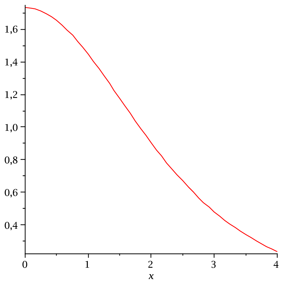
First we will address the massless zero mode case, later in this section we will study the massless case. The massive case will be consider in the next section. Exact numerical solutions could be obtained as show Fig (3).
For the massless case we have
| (59) |
that has the following base of solutions:
| (60) |
with the plus sign (60) is diverging, with the minus sign is converging provided
| (61) |
it is also a non oscillating when , that is fulfilled by the former equation (61) that will be referred as the thin string limit. Note that in the thinnest limit, when the zero mode converges to a constant value
but the coefficient can be normalized in the curved space we are working on.
Equation (54) could be rewritten as a Sturm Liouville equation:
| (62) |
| (63) |
where the eigenvalues are positive and real constants. The operator is self adjoint and the Sturm Lioville problem has solution with boundary conditions
| (64) |
that are of the same kind of condition taken in [11]. Note that the normalization factor comes from , the weight function, so the ortonormalization condition is:
| (65) |
Then the modes could be written in term of a equivalent normalized function in flat space
| (66) |
That is consistent with the normalization used in [11] and [20] for the graviton case, but in graviton case the weight function was instead of .
Maxwell equation (51) will be solved in term of the zero mode only, if we assume that has not dependence on the angular variable
| (67) |
where
| (68) |
here is given by (60) in the thin limit approximation (61) or could be solved numerically from (57).
In the null thickness limit we simply have
| (69) |
As the massless zero mode has a warping factor, to obtain the equations (51), we must introduce the same warping factor to the current (49):
| (70) |
So, using (67) and (70) in (51) we recover completely the 4 dimensional Maxwell equations very close to the 3 brane. In this case the photon is simply the 4 dimensional vector potential multiplied by a warping factor (60) that confines the photon to the 3 brane universe.
To obtain the non zero Fourier modes, , we could write equation (56) using (38) and (58) as:
| (71) |
these equations has the following base of solutions in the thin limit approximation (61):
| (72) |
where the notation has been used for Bessel functions.
These functions are not bounded for , and could not be normalized because integrals in (65) are diverging. They neither can be normalized using the graviton norm as in (35). So massless non zero modes are not localized on the world brane and wanders into the bulk. The massless zero mode is bounded to the 3-brane only if (61) is accomplished. Finally we want to stand out that if (61) is not accomplished, will be an exponential growing factor and the photon wavefunction will not longer be localized on the world brane, and scape into the bulk.


VI Proca Massive Modes and the Corrections to the Coulomb Potential
The orthogonality of Fourier modes implies that equation (50), and therefore (51) and (52) must be solved order by order. The complete solution will be a superposition of the eigenfunctions with eigenvalues and Fourier index
| (73) |
that is slightly more general that (53), and could be understood as a collection of vector potentials, one for each mode, with electromagnetic fields
| (74) |
Then equation (50) with not current term () could be written as
| (75) |
the sign in is what leads to a non normalizable expressions as (72).
Note that we can add to both right and left sides a Proca mass term:
Former equation (76) could be split in similar way to (51) and (52) as
| (77) | |||||
| (78) |
Equation (77) is a Proca equation with 4 dimensional mass for the photon. Equation (78) gives a regularized version of (54) when and is a self adjoint Sturm Liouville equation.
| (79) |
these equations has the following base of solutions:
| (80) |
where the eigenvalues are effective mass term and notation and has been used for Bessel functions
To obtain the first order electromagnetic field complete solution, we must sum over all the Fourier modes , and as (77) and (78) depends on the mass, we must sum also sum over all the masses , or equivalently on the eigenvalues as indicated:
| (81) |
The expression for (80) could be simplified in null string thickness to:
| (82) |
where a more standard notation for Bessel functions has been introduced and and are constants. That expression is quite similar to that for gravitons [11] and domain walls [2][5][26] changing only the type of the Bessel function and the exponent in the warp factor.
In the limit , the solution (82) grow exponentially for non zero . The standard way to regularize this, is to introduce a finite radial distance cutoff where the boundary condition (64) will be imposed for instead of
| (83) |
These boundary conditions, jointly with the normalization condition (65) leads to a discrete spectrum
| (84) |
for enough large and solving for the constants we get:
| (85) |
When the cutoff is imposed the sum in Fourier expansion (81) will be replaced by a sum over because (84) are the only acceptable values of that will lead to renormalizable wave functions as expected by (65).
The normalization (65) of the massive modes, can be calculated using (82),(85), as:
| (86) |
where the asymptotical form for and , was used due to the large factor for large and enough large
When the cutoff is imposed, the sum in (53) and (81) turns out to be over . So it will be used from now on in the rest of this work. Therefore, massive electromagnetic modes have fourier coefficients given by (66):
| (87) |
A Schrödinger equation could be obtained for the massive modes making the change:
| (88) |
that accomplishes
| (89) | |||||
The potential could be found calculating the integral of the Feynman graph at the tree level, for the interchange of a virtual photon between two stationary charges and placed on the 3-brane at in the limit in which the photon energy goes to zero:
| (90) |
where is the spatial 3-distance between the charges, is the Proca mass, is the usual Schrödinger norm and is a polarization factor.
For both massless and Proca photon the polarization factor is:
| (91) |
where the momentum of the virtual photon, is the conjugate Fourier Transform variable to .
Note that (90) takes into account the contribution of the Maxwell or zero non massive propagator and the contribution of the massive or Proca propagator weighted by the squared norm of its wavefunction (88), that is its probability of been found at . Although the norm of the massive modes (87) is infinite, due to the large factor in equation (86), a finite limit could be found by considering the infinite sum in (90).Using that because therefore the correction to the Coulomb potential could be calculated as:
| (92) |
This infinite sum could be transformed into an integral over the masses , using the quantization condition (84) for which:
| (93) |
So we get to an integral over the masses of the modes:
| (94) |
The former integral could be obtained using (86), (87), (88) and (69). Taking either the large or small limit for in (86) we get:
| (95) |
Evaluating (87) at the brane, and using (95) and Bessel identities we simply obtain:
and using the thin limit for the zero mode (69) we obtain:
| (96) |
Note that in the former integral the cutoff factor was simplified, so the result is cutoff independent. Instead of equation (69), equations (60) and (68) could be used, making a Taylor expansion in gives the same result at second order term in perturbative theory. In the sum there is implicit a step factor if we divide and multiply by we get:
| (97) |
That in the limit and making the change of variables
transform (97) into a double integral
| (98) |
that could be calculated changing to polar coordinates with radius and integrating over the area of the upper left quarter of the plane between . So finally:
| (99) |
If we have a non warped, flat space with 5 dimensional spatial coordinates, a would be expected for the Coulomb potential using Gauss law that is coincident with our result.
VII Summary and outlook
In this work, the confinement of electromagnetic field is studied in axial symmetrical, 6D warped World Brane, using recently proposed [20] topological abelian string vortex solutions as background. The field equations were calculated only to first order in perturbative analysis for the vector field. The metric field was assumed to be exact and the solitonic scalar solution was assumed as solitonic background. As the theory is assumed to be axial symmetric and also containing classical electrodynamic or Maxwell theory, we have a invariant theory as in [16] and [17], that allow us to make two gauge U(1) fixings (44) and (45), that is consistent with the topological abelian string solution, and lead to simplifications in the spin 1 fluctuation equations.
There are several conclusions we found throughout this work: 1. There is a massless, spin 1, Fourier zero mode, bounded to the 3-brane universe, with a warping factor in the bulk if the string-vortex is thin enough. The shape of this mode could be seen in Fig(3) from numerical integration, or obtained in the thin string approximation (61) using (67), (60) and (68) even could be simplified to (69) in the null thickness limit .
2. The massless zero mode is consistent with Maxwell equations (51) with an external current warped throughout the bulk.
3. All other modes in the photon expansion (73) are not localized and massive. They follow Proca equations (77).
4. The main conclusion of this work is that the correction to the Coulomb law, produced by the massive modes, in the thin string limit
is:
| (100) |
The expected Coulomb potential for flat 6D spacetime is , but in this case, it also depends on the factor , that could be seen as the radius of compactification of the angular coordinate, and that is the distance at which the metric falls by a factor of due to the warping factor in Randall Sundrum theories. The value of is unknown, and could be in a very wide range, as short as several Planck length [2] up to the experimental limit for Newton potential aroundcm [27]. The value of is also not know, but must be larger than Planck length, and shorter than the experimental limit of validity for the Coulomb law ofcm [29][28]. Experiments to test at short distances the electric Coulomb potential, could be used to establish the existence or not of extra warped dimensions at distances of cm in the near future. That is an increase by a factor of with respect to the actual capacity to observe gravitational effects due to the warping or compactness of extra dimensions.
Observable effects of the correction to the Coulomb potential (100) implies at least a deviation of , because this ensures a new decimal figure that could not be explained by potential alone. In the most optimistic scenario: assuming cm and , in order to obtain an observable change in Coulomb law at a distance of cm (that could be achieve at the LHC) implies that must be greater than cm. But if cm and cm, for a distance of cm then we obtain that so the precision of the Coulomb law could be amazing.
Proca photons has a long history in both theoretical and experimental physics, a striking limit of gr for the photon mass [28] has been set by astronomical measures. As we have seen in the previous sections, most of the photons will correspond to the massless zero mode, that are localized at , just over the 3-brane universe. On the other hand, massive photons are not bounded to the 3-brane universe and wander in the extra dimensions, throughout the bulk, so the probability of catch one of the Proca photons is extremely low. Lab experiments [29] and astronomical measurements [28] limiting the photon mass, assume that all photons has the same small mass. As this is not the case for this model, these mass limits do not apply.
Acknowledgments
This work was supported by CDCHT-UCLA under project 020-CT-2009.
References
- [1] N. Arkani-Hamed, S. Dimopoulos and G. R. Dvali, Phys. Lett. B 429, 263 (1998) [arXiv:hep-ph/9803315]; I. Antoniadis, N. Arkani-Hamed, S. Dimopoulos and G. R. Dvali, Phys. Lett. B 436, 257 (1998) [arXiv:hep-ph/9804398].
- [2] L. Randall and R. Sundrum, Phys. Rev. Lett. 83, 3370 (1999) [arXiv:hep-ph/9905221].
- [3] M. Gremm, Phys. Lett. B 478, 434 (2000) [arXiv:hep-th/9912060]; C. Ringeval, P. Peter, J.-P. Uzan.Phys.Rev. D65 (2002) 044016; Minoru Eto, Nobuhito Maru, Norisuke Sakai.Nucl.Phys. B673 (2003) 98-130.
- [4] B. Bjac, G. Gabadadz´e, Phys. Lett. B 474 (2000) 282;
- [5] L. Randall and R. Sundrum, Phys. Rev. Lett. 83, 4690 (1999) [arXiv:hep-th/9906064].
- [6] W. Naylor and M. Sasaki, Prog. Theor. Phys. 113, 535 (2005) [arXiv:hep-th/0411155]. M. Minamitsuji, W. Naylor and M. Sasaki, Nucl. Phys. B 737, 121 (2006) [arXiv:hep-th/0508093]. J. Garriga, O. Pujolas and T. Tanaka, Nucl. Phys. B 655, 127 (2003) [arXiv:hep-th/0111277]. A. Flachi and D. J. Toms, Nucl. Phys. B 610, 144 (2001) [arXiv:hep-th/0103077].
- [7] K. Akama, Lect. Notes Phys. 176 (1982) 267; V. A. Rubakov, M. E. Shaposhnikov, Phys. Lett. B 125 (1983) 136; R. Jackiw, C. Rebbi, Phys. Rev. D 13 (1976) 339.
- [8] G. Dvali, M. Shifman, Phys. Lett. B 396 (1997) 64; ibid. 407 (1997) 452;
- [9] G. Dvali, G. Gabadadz´e, M. Shifman, Phys. Lett. B 497 (2001) 271.
- [10] R. Guerrero, A. Melfo, N. Pantoja and R. O. Rodriguez,arXiv:0912.0463 [hep-th].
- [11] T. Gherghetta and M. E. Shaposhnikov, Phys. Rev. Lett. 85, 240 (2000) [arXiv:hep-th/0004014].
- [12] M. Giovannini, H. Meyer and M. E. Shaposhnikov, Nucl. Phys. B 619, 615 (2001) [arXiv:hep-th/0104118].
- [13] E. Roessl and M. Shaposhnikov, Phys. Rev. D 66, 084008 (2002) [arXiv:hep-th/0205320].
- [14] I. Olasagasti and A. Vilenkin, Phys. Rev. D 62, 044014 (2000) [arXiv:hep-th/0003300].
- [15] I. Oda, arXiv:hep-th/0103052.
- [16] M. Giovannini, Phys. Rev. D 66, 044016 (2002) [arXiv:hep-th/0205139].
- [17] M. Giovannini, J. V. Le Be and S. Riederer, Class. Quant. Grav. 19, 3357 (2002) [arXiv:hep-th/0205222].
- [18] S. Randjbar-Daemi and M. Shaposhnikov, Nucl. Phys. B 645, 188 (2002) [arXiv:hep-th/0206016].
- [19] Y. Brihaye, T. Delsate and B. Hartmann, Phys. Rev. D 74, 044015 (2006) [arXiv:hep-th/0602172].
- [20] Rafael S.Torrealba, to be published in Gen. Rel. Grav.[arXiv:hep-th/0803.0313]
- [21] H.B. Nielsen and P. Olesen,Nucl. Phys. B 61, 45 (1973).
- [22] Bogomol’nyi E. B.Sov. J. Nucl. Phys. 24, 449 (1976).
- [23] de Vega and Schaposnik, F. A.Phys. Rev. D 14, 1100 (1976).
- [24] R. Guerrero, R. Ortiz, R. O. Rodriguez and R. S. Torrealba, Gen. Rel. Grav. 38, 845 (2006) [arXiv:gr-qc/0504080].
- [25] R. Guerrero, R. O. Rodriguez and R. S. Torrealba, Phys. Rev. D 72, 124012 (2005) [arXiv:hep-th/0510023].
- [26] Petter Callin, Finn Ravndal, Phys.Rev. D70 (2004) 104009 [arXiv:hep-ph/0403302].
- [27] C. D. Hoyle, U. Schmidt, B. R. Heckel, E. G. Adelberger, J.H. Gundlach, D. J. Kapner, and H. E. SwansonPhys. Rev. Lett. 86, N∘8, 1418 (2001)
- [28] Roderik Lakes, Phys. Rev. Lett. 80, N∘9, 1826 (1998)
- [29] E. R. Williams, J. E. Faller, and H. A. Hill ,Phys_ Rev_ Lett_ 26, 721 (1971)