Strings on Bubbling Geometries
Hai Lin11 1 e-mail: hai.lin@usc.es, Alexander Morisse22 2 e-mail: alexander.morisse@usc.es and Jonathan P. Shock33 3 e-mail: shock@fpaxp1.usc.es
Department of Particle Physics, Faculty of Physics,
University of Santiago de Compostela, 15782, Santiago de Compostela, Spain
We study gauge theory operators which take the form of a product of a trace with a Schur polynomial, and their string theory duals. These states represent strings excited on bubbling AdS geometries which are dual to the Schur polynomials. These geometries generically take the form of multiple annuli in the phase space plane. We study the coherent state wavefunction of the lattice, which labels the trace part of the operator, for a general Young tableau and their dual description on the droplet plane with a general concentric ring pattern. In addition we identify a density matrix over the coherent states on all the geometries within a fixed constraint. This density matrix may be used to calculate the entropy of a given ensemble of operators. We finally recover the BMN string spectrum along the geodesic near any circle from the ansatz of the coherent state wavefunction.
1 Introduction
The AdS/CFT correspondence is an invaluable tool [1], not only enabling us to study the strong coupling limits of a wide variety of gauge theories, but also allowing us to study deep questions arising in the study of quantum gravity.
Certain heavy supersymmetric states in the gauge theory can be dual to geometric backgrounds in string theory. An example is the set of 1/2 BPS chiral primary states built with one complex scalar [2],[3],[4],[9],[10]. These operators can be labelled by Young tableaux or Schur polynomials which themselves form an orthonormal basis. When the charges of these operators are very large, they become dual to a variety of geometries, which have bubbling type boundary conditions in some loci of the spacetime far from the boundary, that encode the mapping from the gauge theory states. Besides the 1/2 BPS chiral primary operators, there are also other types of operators with corresponding bubbling geometries, e.g. [11],[12],[13],[14] in SYM.
A natural question which arises is what is the description of the non-BPS excitations on top of the above states in both the gauge and string theory sides? On the gauge side, we study operators which are products between a Schur polynomial and a single trace operator. We may view the Schur polynomial as the background geometry and the single trace part as a further stringy excitation on the geometry. On the string side, we study closed strings excited on the dual geometries, described by a general Schur polynomial or Young tableau. In particular we study the backgrounds with general concentric ring distributions [4] in the phase space plane. The size of the ’s in the LLM metric are determined by the position in the droplet distribution, in which the edges correspond to the vanishing of one or the other .
One way to study such non-BPS states is to look at the dilatation generator acting on them. The dilatation operator acting on the non-BPS state is naturally described in terms of the hamiltonian on a lattice, which itself can be described in a variety of limits. The bosonic occupation numbers of the lattice sites correspond to the number of complex scalar fields in the trace part of the operator in between the impurity fields. This has been studied before in the context of certain background geometries [5],[6],[7],[8]. We will be particularly interested in studying the coherent states of such a lattice, though for more general background geometries. In the continuum limit of the lattice we obtain a sigma model that matches with the sigma model of the closed string living in the dual geometry. We can also study the lattice with a small number of sites, corresponding to short BMN type strings.
In [6] an analysis was made of a reduced subspace of possible diagrams. In this work the authors analyzed the coherent state on a disk plus ring distribution and proved that the normalized wavefunction constructed from this coherent state knew about the geometry and topology of the string theory background. In the current work we fully generalize this description to include any geometries which can be described by axially symmetric solutions in the phase space plane.
Furthermore we will look at the entropy of particular ensembles of such states. In the 1/2-BPS limit all non-equivalent geometries are orthogonal to one another, meaning that an ensemble made of such solutions does not mix. The breaking of supersymmetry via the stringy excitation/trace operator allows for a mixing between elements of the gravitational ensemble and a non-diagonal reduced density matrix.
The organization of this paper is as follows. In section 2.1, we introduce the non-BPS operators that we will study, the lattice labelling, and the associated oscillator algebra. In section 2.2, we analyze the coherent state wavefunction of the system, the continuum limit of the lattice and sigma models, and also the properties of the coherent state wavefunction, such as the norm and the average occupation number. In section 2.3, we describe a density matrix over these coherent states with a constrained set of Young tableaux, and from this we are able to calculate the entropy of such an ensemble of states. In section 2.4, we derive the BMN states from the ansatz of the coherent states and show that in the appropriate limits we recover the results of [6]. Finally, in section 3, we briefly discuss our results and conclude. We also include four appendices providing concrete computational details on the calculations discussed in the body of the text.
2 Strings on Bubbling Geometries
2.1 Operators
The 1/2 BPS chiral primary operators of super Yang Mills can be labelled by Schur Polynomials , where is the representation in which the operator is being traced, and is one of the complex scalar fields. Equivalently they can be represented by Young tableaux which are dual to BPS geometries. These can be described using the LLM prescription as a series of concentric black and white annuli distributions. The Young tableau corresponding to a particular chiral primary operator may be labelled by the positions of its corners. We label outward corners with a “” and inward corners with an “”, going from bottom left to top right. A given diagram will come with labels where is the total number of inward, or equivalently outward pointing corners. Such operators can be mapped into a distribution of black rings where the inner and outer edges of a ring/annulus correspond on an outward pointing or inward pointing edge of a Young tableau, respectively. We label these inner and outer radii as and where labels the ring (we will use and to label ring numbers throughout). Due to quantization of the phase space area, the radius squared of each inner circle of the black rings is proportional to the distance from the lower-left point of the Young tableau to the outward corner , of the Young tableau, counting along the edge. Similarly, the radius squared of each outer circle of the black rings is proportional to the distance from the lower-left point of the Young tableau to the inward corner 44 4 The coordinates of the -plane in this paper are rescaled from the coordinates of the -plane in [4] by a factor, such that :
| (2.1) | |||||
| (2.2) |
This provides a simple mapping between a Young tableau labelling and a phase space distribution.

It should be noted that such Young tableaux do not exhaust all possible concentric ring distributions. Such a description will not include phase space distributions which start with a black disk55 5 These would correspond to limit, which will be discussed more in Appendix A.. These are labelled separately with a thin vertical line running from the bottom left hand corner of the Young tableau, corresponding to having no white region in the centre. The labelling of such states follows logically. The bulk of this paper is motivated by studying closed string states in backgrounds given by general axially symmetric ring distributions.
Having described this subspace of the half-BPS sector we would like to look at products of a trace multiplied by an operator described by the Schur polynomials discussed above. Such products are in general non-BPS and we will utilize the breaking of supersymmetry in what follows. We label such products as:
| (2.3) |
where is a Schur polynomial corresponding to a Young tableau of representation . is a letter corresponding to impurities coming from fields which are not in the 1/2 BPS chiral primary sector. is a field creating or removing a box with weight or at the Young tableau corner, where the subscript denotes the corner or (see also [7]). Such an operator corresponds to a closed string, represented by the trace, in a background represented by the Schur polynomial. The presence of the string in the background leads to SUSY breaking. The operators that are eigenstates of the dilatation operator are superpositions in the space spanned by the basis (2.3). (In [6], product of determinants were used in place of the Schur polynomial part.) The total number of s in the trace part of (2.3) is not fixed when we mix these operators to obtain the eigenstates of the dilatation generator, so it is convenient to view the trace part of (2.3) as a lattice of sites each with an occupation number . For simplicity, we first take to come purely from the complex scalar . Each operator can thus be represented by a state The positive occupation number corresponds to positive angular momentum of the string along the outer circle of a black ring, while the negative occupation number corresponds to the negative momentum of the string along the inner circle of the black ring. Such a basis can be used to describe a wide variety of string states in 1/2-BPS backgrounds.
The effective Hamiltonian of the lattice is derived from the dilatation generator , where
| (2.4) |
for the operators under consideration, and here We have
| (2.5) | |||||
| (2.6) |
where in the last line we only consider the one-loop dilation generator. The Hamiltonian when acting on the lattice takes the form
| (2.7) |
where are shift operators which reduce the bosonic occupation number by one. We use to denote the total -charge associated with and use to denote that -charge from the trace part, i.e.
| (2.8) |
For a general Young Tableau, we have the following algebra
| (2.9) | |||||
| (2.10) | |||||
| (2.11) | |||||
| (2.12) |
The state corresponds to the excitation on the inner edge of the ring while corresponds to the excitation on the outer edge of the ring. As noted before, the and are the distances (number of boxes) between the outward pointing or inward pointing corner and the bottom-left point of the Young tableau. The and are also the weights of the boxes of these Young tableau corners, and are the coefficients that appear in the two-point correlators for the fields [7]. The action of the annihilation/creation operator on different types of field excitations differ by the coefficients , or , and is otherwise similar. The action of () removes (adds) a box in the appropriate corner of the Young tableau. More discussions of their properties are included in Appendix A.
In principle one can take several limits in order to study superpositions of operators of the form (2.3), and their string theory duals. The limits of interest (both on the gauge and string side) include:
1. The continuous limit/sigma model limit:
| (2.13) |
2. The BMN/plane-wave type limit:
| (2.14) |
3. The Hofman-Maldacena type limit:
| (2.15) |
where in the last two cases, we use a
two-site lattice, corresponding to a two-magnon state. It is of course possible to study this in a more general -site lattice.
2.2 Coherent String States
We would like to be able to describe a coherent string state on the background given by an arbitrary distribution of black rings, as discussed in the previous section. In order to be able to do this we find a coherent string prescription which is normalizable on each of the black rings separately. The coherent state satisfies the equation [23]
| (2.16) |
where the labels the ring in which the wavefunction is well defined and normalizable.
The coherent state can be expressed as
| (2.17) |
which is normalizible on the black ring, i.e. . The state corresponds to the excitation on the outer edge of the ring while corresponds to the excitation on the inner edge of the ring. It can be shown that the sums over can be consistently restricted to the ranges in (2.17) due to the normalizability on the ring. A more detailed derivation of the above is included in Appendix A.
In (2.17), we sum over all the positive occupancies, or in other words, positive angular momentum movers along the outer circles, outside the black ring, and over all the negative occupancies, or, negative angular momentum movers along the inner circles, inside the black ring. Note that such a summation is important for normalizability within the ring. The coefficients and correspond to the relative contribution to the wavefunction from the excitations associated with the and circles. Equivalently these circles correspond to the corners of the Young tableau from the gauge theory point of view.
(2.17) is a Fock space state which sums over all occupation numbers, as well as all types of oscillators specified by the Young tableaux corners . The real, positive coefficients can be shown to satisfy the following relation
| (2.18) |
where is a mixing matrix which allows for mixing between different rings. The can then be written as
| (2.19) | |||||
| (2.20) |
| (2.21) | |||||
| (2.22) |
where we have used the identity (2.1) to write these expressions in terms of . It can be shown that these expressions are positive definite.
By looking at the behavior of the norm when merging two black rings, we get
| (2.23) |
where is an overall normalization which is unfixed from the coherent state condition but will be fixed later by putting a constraint on the integral over the inner product of such representations in the -plane. Finally, one can write the coherent state wave-function on the entire -plane as a sum over the states defined on each ring:
| (2.24) |
where has unit support between and , and is 0 otherwise.
Having defined such a coherent state on the 1/2 BPS background, one can take the continuum limit:
| (2.25) |
as the product of coherent states on each lattice site:
| (2.26) |
This limit would correspond to the large angular momentum () limit on the string side. A general coherent state is then labelled by a coherent state on each site of the lattice:
| (2.27) |
The continuum limit can be expressed in terms of a sigma model action with Hamiltonian (2.7), which is derived by looking at the large limit of the lattice action:
| (2.28) | |||||
| (2.29) |
This is a sigma model with target space the -plane of the 1/2 BPS bubbling chiral primary geometry [5],[6], see as well [7]. This Landau-Lifshitz type action coincides with the action from the string theory side for the string sigma model that describes a closed string traveling with large angular momentum on the in the 1/2 BPS bubbling geometry under the uniform gauge, in which the angular momenta on the are uniformly distributed along the string. This uniform gauge corresponds to the uniform distribution of the fields on the lattice sites. This action can be written in terms of the above potential as:
| (2.30) | |||||
| (2.31) | |||||
| (2.32) |
| (2.33) |
We have neglected higher order terms , which would correspond to the contribution from the two-loop dilatation operators and can be safely neglected in this limit.
The equations of motion coming from this action are
| (2.34) |
which have static solution
| (2.35) | |||||
| (2.36) |
where are constants of motion, and the solution corresponds to a straight string stretching across a black ring (and back again).
One can also bring (2.30) into the canonical form of a 2d complex scalar field theory. We can transform the bringing the kinetic term into its canonical form
| (2.37) | |||
| (2.38) | |||
| (2.39) |
Under this transformation, the complex scalar field theory is described by the action
| (2.40) |
where
| (2.41) |
The potential terms in this action are dependent on the background in which the string is moving. This means that the action is dependent directly on the droplet configuration in the -plane. In particular the topology of the background which is related to the number of inner and outer rings is captured in the potential. One can study the S-matrix of this model, via similar methods to [16] for . For example for the case the potential is given by:
| (2.42) |
| (2.43) |
maps the disk into a whole plane and is the radius of the disk. For more general concentric black-ring configurations we have
| (2.44) |
The limits of such an expression can be found in Appendix A.
We would now like to derive such a potential from the coherent state. We first consider the norm of the coherent states The coherent state (2.17) defined on the ring is:
| (2.45) |
where
| (2.46) |
which have the property
| (2.47) | |||||
| (2.48) |
From the coherent state expansion we get
| (2.49) |
which leads to a relation between the coefficients in the coherent state expansion
| (2.50) |
Note that the coherent state norm is nonzero only on the black rings. The expression (2.49) can be summed and factorized in the numerator, and rewritten as
| (2.51) | |||||
| (2.52) |
The norm of the coherent state can also be written in terms of the potential, , as
| (2.53) |
which can be used to calculate the potential:
| (2.54) | |||||
Note that the existence of is consistent with the existence of an integration constant in (2.53).
The coherent state norm is non-zero only on the black-rings as the potential diverges at their edges. This calculation of the potential matches with the function derived in the sigma model from the string theory side. This shows that the coherent state wavefunction knows about the geometry of the multi-ring background. Moreover, the coherent state wavefunction has a different expression on each disconnected black ring, meaning that it knows about the disconnectedness of the droplets, topology, of the background.
Another property we can study using the coherent state we have described above is the average value of the occupation number on each lattice site. From (2.17), we have the coefficients in the coherent state expansion expressed as
| (2.55) |
The states are orthonormal, such that
| (2.56) |
Excitations of a different level or on a different ring are orthogonal.
The coherent state is a superposition of states with different occupation numbers so in order to find the average occupancy we have to look at the probability of occupancy or on a given inner or outer ring. For the inner rings the probability of occupation number on the ring is given by:
| (2.57) |
and the average occupation number on the inner edge of the ring is (for )
| (2.58) |
Similarly for the outer edge of the ring we have a probability of occupation number :
| (2.59) |
and the average occupation number on the outer edge of the ring is (for )
| (2.60) |
We can now define an occupation number operator . The average occupation over all inner and outer rings (corresponding to the average charge on the string) for the entire coherent state is
| (2.61) | ||||
| (2.62) | ||||
| (2.63) |
where the norm can be written as
| (2.64) |
So we see that
| (2.65) |
which is again a quantity depending on both the position of all the black rings, and on the ring from which the measurement is being made. The average occupation number gives the average charge of the single trace part of the operator (2.3),
| (2.66) |
and also gives the average angular momentum of the string on the -plane.
2.3 Density Matrix
The states we consider in (2.3) are in general non-BPS states. They are dual to strings on the bubbling AdS backgrounds described by systems of concentric rings in the LLM plane. In the situation where we have only the 1/2-BPS backgrounds, all distinct representations (described by the Schur polynomials) form an orthonormal basis. Having broken supersymmetry with the inclusion of the trace operator, such orthonormality is however no longer guaranteed. Let us consider two very similar background geometries which have a large number of identical coincident black rings and a small region where the ring structures differ. The coherent state wavefunction will be able to distinguish such small differences. The radii, defining a given ring configuration (2.17), can be viewed as the continuous parameters in the coherent state string wavefunction, and we can study the entire class of background geometries from the point of the view of this wavefunction.
Having obtained the coherent string state on a general background geometry given by a Young tableau representation , we can write the string state in this background as
| (2.67) |
where labels the background geometry, and is seen in the set of parameters in the coherent state wavefunction (the ). There are various constraints we may place on the representation but for now we study representations with fixed total number of boxes and total rows. We would like to define a reduced density matrix by studying the inner product between different string states in different backgrounds (representations ) and then integrating out the string degrees of freedom. This can be achieved through the following definition of the reduced density matrix over coherent states,
| (2.68) |
where because of the functions in the definition of the only contributions to the integral come from the regions in the LLM plane where the black regions in the representations and overlap. The wavefunctions are normalized (using the integration constant in (2.23)) such that the reduced density matrix element of one representation with itself is unity,
| (2.69) |
Given a particular constraint on the representations (a constraint on the total number of boxes, rows and columns) we can define an entropy by looking at all possible inner products between representations within a superselection sector. The entropy of such a system is given by
| (2.70) |
where In other words we take the trace over the space spanned by the Young tableaux basis (including the additional Young tableaux plus black inner disk configurations).
Looking at a fixed total number of boxes and a fixed number of rows , if we define the number of Young tableaux with no coincident radii as , and the total number of Young Young tableaux as the entropy will be between log and log We can also put a constraint on the density matrix in terms of the size of the off-diagonal components. The diagonals of the density matrix are equal, due to the normalization described above. We define the density matrix as the addition of the diagonal part and an off-diagonal part ,
| (2.71) | |||||
| (2.72) |
where is the total number of Young tableaux. This density matrix measures the similarities of different Young tableaux, and due to the contribution from the off-diagonal components, the entropy gets reduced from log If the Young tableaux are all identical then the entropy reduces to zero, and the system becomes a pure state. If on the other hand, the off-diagonal contributions are small, which is the case for (a sparse distribution of rings with many large gaps), then the entropy is close to log; in that case the second term in (2.72) can be approximated as . We analyze the dimension of a constrained set of partitions in Appendix B.
In general we constrain the Young tableaux to have fixed and fixed .
In order to calculate the reduced density matrix we must understand the inner product between two non-equivalent representations. Consider the two coherent string states in the backgrounds with representation and with and total black rings respectively. The coherent states are defined as:
| (2.73) |
| (2.74) |
The inner product between the two representations can be written in terms of a contribution from the inner edges and outer edges separately as there are no cross-terms between ’s and ’s:
| (2.75) |
Looking at the type contributions we find the following set of summations:
| (2.76) | |||||
and similarly for the type contributions
| (2.77) | |||||
The calculation of such an inner product is complicated both by the large numbers of summations in the above terms, and also by the products implicit in the . Having calculated the inner products the integration must be implemented. The integration itself is not complicated but because there are very many terms we have performed all such computations using Mathematica. In order to find the full reduced density matrix it is also necessary to find all the possible Young tableaux for a given set of constraints. We also do this using Mathematica. The algorithmic procedure is outlined in Appendix C while an analytical estimate of the dimension of the reduced density matrix is given in Appendix B. The dimension of the reduced density matrix for , is greater than 800 meaning that there are about a million non-equal entries in the density matrix. Such a computation is possible but, for representations with and much greater than 10, the combinatorics very quickly become unmanageable, .
In the following we plot some of the results for various and , noting that for and of order 10, we can consider that we are approaching the large regime.
For there are 29 distinct representations (the representations are given in appendix C). The reduced density matrix can be diagonalized and the logarithm of the 29 eigenvalues calculated. The non-diagonalized reduced density matrix along with the logarithm of the eigenvalues are plotted in figure 2. Note that if there were no mixing, all eigenvalues would lie on the dashed line.


In figure 5 we plot the entropy as a function of and for .
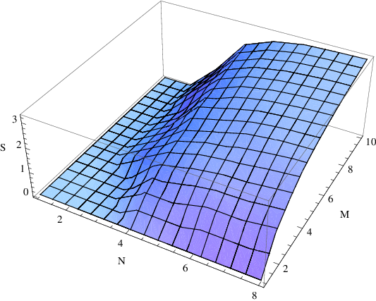
We see that for large and the entropy goes much slower than log meaning that the off-diagonal elements are extremely important in describing the purity of the state. Indeed the constraint we are looking at and is one in which we would expect a large number of overlaps in diagrams. This means that, in this case, the number of degrees of freedom is actually much less than the dimension of the density matrix.
The limit of small , large , however gives a result much closer to as can be seen in figure 6 where the points are the values of the entropy calculated for and the line is given by , showing an almost perfect match in this limit of no overlaps. Note that there is a subtlety in such a calculation which is dependent on how one regularizes the divergences in the reduced density matrix. See Appendix C for more details.

2.4 BMN String States
Having studied the continuum limit, we turn to the two-site lattice in the BMN limit.
Such states can be viewed as the two-magnon states of the string with large charge. We can project onto states with fixed angular momentum by performing the contour integral over the product of two coherent states as follows:
| (2.78) |
however unlike in the one black-ring case [6], is a sum of contributions from each ring, so we have to sum over rings:
| (2.79) |
where is the theta function with unit support only on the ring (this is simply a rewriting of (2.24) without referring to the ring radii).
Since we are only looking at a single representation, , (both s are the same), the product of means that the above simplifies to:
| (2.80) |
We therefore start by looking at
| (2.81) | |||||
Only terms which have a single negative power of will contribute to the integrand. Therefore, for positive this is only possible for terms of the form , , and . There will be no contributions from a product of two negative movers (two types) only.
Calculating the contribution from each and summing we arrive at the final expression for the angular momentum eigenstate as:
| (2.82) | |||||
The analysis for the total negative states is similar, except that we now pick up products of two type states, and do not pick up the products of two type states.
We can now use (2.82) as a general ansatz to write down an energy eigenstate. Simplifying this expression we arrive at,
where we write the two occupation numbers together into one bracket and leave the information about which ring is being excited as a subsript after the ket. The are calculated after applying an energy eigenstate constraint on the kets. A full explanation of this procedure can be found in Appendix D. In order to find the correct constraints on the we have to simplify the problem by looking at a decoupling limit which reduces us to the two site case already discussed extensively in [6]. The full problem of finding the in complete generality is outside the scope of the current paper.
The decoupling limit which we choose is the one in which a single black ring, the is decoupled from the rest. In (2.4), we pick and since and we can define and the state and algebra are very similar to the one black ring case [6]. From the general expression (2.4), we get in the decoupling limit that
| (2.84) |
where .
The energy eigenstate equation is
| (2.85) |
i.e.
| (2.86) |
Applying this operation to our state we get:
This equation generates recursion relations between triples of and we can solve the whole system iteratively starting from just two e.g. . These recursive equations will be almost the same as [6], except that in () we have instead of . We thus have three unknowns, is set to 1 via an overall normalization freedom while and are fixed by demanding convergence of the series in the two asymptotic regimes . The calculation is discussed in detail in the appendix but the outline is the following: Three generating functions are derived which describe in closed form the recursion relations between and , and and, and . Using these generating functionals we are able to write and in as functions of and . Convergence of the sums puts a constraint first on from the regime and finally a constraint equation is found for from the regime. More detailed discussions are in Appendix D. One finally gets that for large states, the eigenvalues are 66 6 The state is equivalent to the state under a cyclic permutation of the integers, e.g. to [6], due to the cyclicity of the trace part of the operator (2.3). For a two-site system, one can write a general state as the sum of a symmetric state, i.e. one with the property , and an anti-symmetric state, i.e. one with the property . The energy eigenstate equation (2.86) is to be supplemented by the projection onto symmetric eigenstates. Thereby one should project out half of the eigenfunctions of the equation, associated with , and only keep the other half with [6], and interpret the as the mode number of the BMN state. Therefore finally (2.88), (2.89) are in agreement with [6].
| (2.88) |
where here , and is the oscillator mode number in the BMN state [15]. A similar procedure for large states produces similar recursive relations and yields
| (2.89) |
These are strings excited along the exterior and interior edges of the black ring. The different coefficients in the energy spectrum reflect the different effective radii of curvature when we take the plane-wave limit along the geodesics near the different circles [4]. Thus, by measuring and comparing the effective units of energies of the states, one can know the exact location of these (short) string excitations in the bulk spacetime.
3 Discussion
In this paper we have studied the quantum string excitations on top of a class of axially symmetric bubbling geometries dual to the 1/2 BPS chiral primary operators. This work is a continuation of the research undertaken in [5],[6],[7],[8]. On the gauge theory side, we have studied operators of the form of a product of a Schur polynomial and a single trace of and impurities . The Schur polynomial part corresponds to a general Young tableau which specifies a background geometry. The single trace part can be viewed as a bosonic lattice of and for each site there are, in general, type of bosonic excitations, of which have positive occupation numbers , corresponding to the inward corners of the Young tableau, at which point one can add extra boxes there. The other , with negative occupation numbers, , correspond to the outward corners on the Young tableau, where one can subtract boxes.
Developing the work of [5],[6],[7] we have solved the problem of the coherent state for a general geometry with arbitrary concentric ring distributions (i.e. a general set of radii), and equivalently for a general Young tableau.
We have also studied the algebra of the shift operators (or ladder operators) , acting on the different types of bosonic excitations on the lattice, and extended the algebra of [7] by including the mixing of the states of different black rings. These different types of excitation correspond to the different possible circles in the geometry. The coherent state wavefunction has different expressions on the different and disconnected black rings. On each black ring, the contribution to the Fock state wavefunction, normalizable on that ring, comes from all the positive mover states along the circles outside that ring, and all the negative mover states along the circles inside that ring.
The norm of the coherent state wavefunction is related to the metric function that appears in the dual string sigma model [5],[6],[7]. The radii that appear in the denominator of the norm are those radii for which the angular momentum excitations of the string are included in the coherent state expansion. The radii that appear in the numerator of the norm are all the rest of the radii in the geometry, and emerge due to the factorization of the numerator after summation. We have also calculated the average occupation number on each black ring, which are related to the metric function . We have checked that the coherent state wavefunction behaves nicely under the merging of two nearby rings.
Having obtained the coherent state wavefunction for a general concentric ring geometry, or equivalently, for a general Young tableau, we used the wavefunction as a means to study the different background geometries since the continuous parameters of these geometries are encoded in the coherent state wavefunction itself. We have then gone on to define a reduced density matrix element between any pair of geometries or Young tableaux. This has been implemented by integrating out the string degrees of freedom from the cross product between the coherent state wavefunctions living on these geometries. The reduced density matrix measures the degree of similarity between any pair of geometries. In the most extreme case, if the two geometries are almost identical except for some very small inequivalent region, the matrix element between them is close to , where is the total number of Young tableaux in a given constrained ensemble. We use computational methods to obtain both the representations in the ensemble and furthermore the reduced density matrix itself. This calculation is a novel development, which allows us to study the mixing of non-supersymmetric operators. The mixing of the tableaux is due to the non-BPS property of the entire operator (Schur polynomial times single trace).
We have also studied an ansatz similar to the coherent states that describe the BMN states with large charge. The coherent state has no fixed total , but includes a superposition of all states with different . By picking the fixed solutions from within the coherent state expansion, and using these states as the basis for the superposition to form a BMN eigenstate of the dilatation generator, we are able to solve the eigenvalue problem and find the eigenvalues. The spectrums encode the different radii of the rings within the geometry and therefore the locations of short string excitations in the bulk gravity dual. It therefore tells us some locality information of the bulk quantum gravity. We also show that one can obtain the BMN states with large negative charge, which correspond to the negative movers along the inner circles of the different rings. For fixed large , the number of sites of the lattice corresponds to the number of magnons on the string.
In finding the string sigma model in these geometric backgrounds we obtain a metric function, , which describes the entire class of concentric ring geometries. The metric function is a superposition of many terms each of which looks like a metric function for an space with a different radius. A future goal would be to consider the solutions, and S-matrices of these sigma models in more detail. The straight string solutions are of particular interest, and may be related to the work of [24], [25]. Semi-classical long strings on these backgrounds were studied previously in [26]. It would seem natural to consider these as operators of the form of the product of the Schur polynomial and an additional operator.
A further direction of research would be to consider the higher loop dilatation generators acting on the lattice, having here extensively studied the application of the one loop dilatation generator. It would also be interesting to generalize the trace operator under consideration from one which contains only and impurities to one which contains fields from a larger sector, for instance the derivative operator. There is still much to be done to fully understand many aspects of these types of operators.
Acknowledgments
This work is supported in part by the ME and Feder (grant FPA2008- 01838), by the Spanish Consolider-Ingenio 2010 Programme CPAN (CSD2007-00042), by the Juan de la Cierva program of MCyI of Spain, and by Xunta de Galicia (Conselleria de Educacion and grants PGIDIT06 PXIB206185Pz and INCITE09 206 121 PR). H.L. also would like to thank Bin Chen, Bo Feng, Oleg Lunin, Juan Maldacena for some correspondences, and University of Chicago, McGill University and CERN for hospitalities. AM is supported by FCT grant SFRH/BPD/65058/2009. A.M. also would like to thank the University of Santiago de Compostela for their hospitality.
Appendix A Derivation of the coherent states
Here we give a more detailed explanation of the calculation of the coherent state, used extensively throughout this work.
We assume that the coherent state on the ring takes the form
| (A.1) |
where the excitations on the inner and outer rings are labelled by and and the ground state of the ring is labelled by . The ranges of the sum over is due to the normalizability on .
The algebras are written in section 2.1, and in particular, we assume that the action of the annihilation operators on a single positive mover gives a sum over zero modes:
| (A.2) |
The mixing of the states is natural, since when two nearby black rings merge, or equivalently, two nearby vertical edges of the Young tableau merge together, the states on these two black rings, under this limit, have to be identified as the same state. The algebra without such mixing would reduce to decoupled algebras, each of which has a similar form but with different coefficients.
We then have that the action of the annihilation operator on the negative and positive movers respectively gives
| (A.3) |
| (A.4) |
The coherent state condition then needs to be satisfied which will provide a series of recursion relations for the . The condition
| (A.5) |
yields the constraint
| (A.6) |
which gives a relationship between the and
| (A.7) |
We also have the following constraint coming from the sums over zero modes
| (A.8) |
which can be rewritten as
| (A.9) |
and thus
| (A.10) |
Taking the above constraints we are left with a simplified expression for the coherent state, given by:
| (A.11) |
where we have made a choice to absorb the zero modes in the states. From the coherent state expansion we get the norm of the state on the ring as
| (A.12) | |||||
| (A.13) |
which can be re-summed and factored in terms of a quotient of products as
| (A.14) |
where is an overall normalization constant.
Since when there is no black region in the center, the norm is zero when :
| (A.15) |
which has solution
| (A.16) | |||||
| (A.17) |
| (A.18) | |||||
| (A.19) |
where sign for ; and sign for .
It can be seen that
| (A.20) | |||||
| (A.21) |
The and coefficients give the relative strengths of the response of the ring to the excitations on , circles in the -black-ring geometry.
It can be checked that they correctly produce all the non-zero coefficients of the 2-circle case with
| (A.22) |
since is already proportional to and we use the coordinate in the units that is 1.
It can also be checked that they correctly produce all the non-zero coefficients of the 3-circle case with
| (A.23) |
These match with the 3-circle result in [6]77 7 There is a slight typo in equation (58) of [6], where the prefactors of the last two terms are switched.. Note our 4,3,2 is their 3,2,1, we have taken the limit, and these normalizations make the norm of coherent state when to be 1 (in the unit of ) at the origin, . In this procedure, we first take then .
From this one can calculate the coefficient , giving
| (A.24) |
where the subscript on denotes the representation and not a radius. Before taking the limit the expression has the property that the coherent state wavefunction is normalized to zero at the origin, because there is no black region there. The limit from circles to circles is similar.
The overall normalization factor for each black ring has the property that:
| (A.25) | |||||
| (A.26) |
When one crosses from the ring to the ring, there is only a change of factor
| (A.27) |
Similarly, when one crosses from the ring to the ring, there is only a change of factor
| (A.28) |
These are due to the sign changes of the contributions in from the two circles that one passes by.
The disappearance of the central circle leads to the limit
| (A.29) |
which gives a good limit to the case of an odd number of circles - i.e. a disk plus annuli configuration. This is also a good limit for , since .
A merging of two black rings when is also a natural and well behaved limit, as, e.g.
| (A.30) |
so the formula reduces to the situation with one fewer black ring. This is also a good limit for , since , and contributions from the two merging circles cancel.
The situation where the black ring is far away from others leads to the following limit
| (A.31) |
which reduces to the one black ring case, which is a form of decoupling limit for the ring.
The limit where we go from circles to circles takes the following form
| (A.32) |
In fact the 2-circle case can be viewed as a limit of the 3-circle case with leading to the term.
There is a further limit which would give the wavefunction in complimentary regions nomarlizable on the white regions instead of the black. Starting from the case of an even number (e.g. ) of circles, and sending the last circle to infinity, followed by switching the black and white regions leads to
| (A.33) |
This procedure gives us coherent state wavefunction in white regions instead of black, as it is complimentary to the wavefunction in the black regions.
Appendix B Dimension of the density matrix
The dimension of the density matrix in section 2.3 is related to the entropy of the superstar, via
| (A.34) |
The superstar geometry corresponds to a grey disk on the -plane with a larger radius and lower fermion filling density than the AdS disk. It has the same as the AdS geometry but has a larger radius on the -plane [4],[17],[18]:
| (A.35) | |||||
| (A.36) |
A single superstar may be viewed as a microcanonical ensemble with total rows, and total columns, both fixed. In other words, we have
| (A.37) |
The slope of such a Young tableau is, in the limit of large and ,
| (A.38) |
and the filling density on the grey disk with the larger radius, is .
One can consider the entropy as the sum of entropies of each area element in the phase space, each of which is subject to a Bernoulli distribution . The sum is written in [19] (see also [20]) which is
| (A.39) | |||||
| (A.40) |
where the area is quantized due to the quantization of the phase space
| (A.41) |
(see the footnote on page 3). For a uniform distribution in the phase space, is a constant which is the filling fraction , and we can thus write the entropy as
| (A.42) | |||||
| (A.43) |
where
| (A.44) |
This agrees exactly with [18], which is derived from the partition function approach.
In the case of unrestricted and , the Hardy-Ramanujan formula tells us that [21],[18]
| (A.45) |
on the other hand from (A.43)
| (A.46) |
which is consistent with the Hardy-Ramanujan bound.
In the regime (A.43) has the limit,
| (A.47) |
This formula is similar to the case of the type IIA geometry with units of D2-brane flux and units of NS5-brane flux on the torus [22].
Another method to obtain this order of magnitude estimate for the entropy in the superstar geometry is by using Schur’s theorem to find the number of partitions of with maximum rows. If denotes the number of possible sets which satisfy the relation and are non-negative, and are relatively prime, then
| (A.48) |
in the large limit. This should give an order of magnitude estimate, with the distinction coming from the fact that the set may not be relatively prime. If we let , which is the case we are interested in, we find
Appendix C Procedure for computing the density matrix
In this section we will give a detailed explanation as to how to calculate the reduced density matrix given a set of Young tableaux. We start with two representations shown in figure 7. The two ring configurations for the representations and are drawn only in their half planes so that we may see the coincident outer rings (marked with black lines) and coincident inner rings (marked with dashed blue lines).
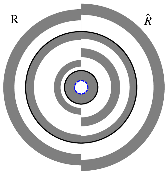
We may draw a more detailed picture of these two representations by simply plotting the radii in a linear fashion, as shown in figure 8. In this figure we have also labelled the and oscillators for the representation along with the eight radii and similarly the and for the representation.
We see that the ring radii are coincident on two outer rings and one inner ring (the innermost). Note that the actual values of the radii are unimportant for this example. We simply aim to show the calculational procedure.

We first write the coherent state wave function for the first ring structure (which has four rings) as:
| (A.50) |
and for the second
| (A.51) |
where each coherent state wavefunction has support only on the ring for and zero otherwise. Note that these are coherent states, though we can multiply the whole state by an arbitrary constant and it will still be a coherent state. We set this arbitrary normalization such that the inner product of the state with itself, integrated over the whole space gives where is the total number of representations in the ensemble.
| (A.52) |
We can write out the coherent state wavefunction in full, in terms of the defined in (2.22)
| (A.53) |
| (A.54) |
Note that the fact that there are four rings in both representations is a coincidence - in many cases one looks at the overlap between representations with different numbers of rings.
Now let’s look at the inner product of these two objects. There is one clear simplification we can make. This is that there are never any cross products between the ’s and the ’s, so we can write:
| (A.55) |
Looking first at the contribution in (A.55) we see that we have the following sums:
There are two positions where the outer rings overlap, for and . Note that it does not have to be the case that they are on the same rings. From this observation we get the following two terms contributing:
| (A.57) | |||||
The first term includes a contribution from only one ring, whereas the second term, which comes from coincident ’s on the third ring gives contributions from all the overlapping regions of all inward rings from that point.
We can write a similar expression for the ’s and we find that the process is very similar except that the contribution comes from all rings out from the coincident radii. This time there is clearly no contribution from the second rings as they do not overlap at all, so there are again just three contributing terms here
| (A.58) |
Note that it is just a coincidence that the radii have the same label in the products of ’s - they may come from overlaps of very different ring numbers in more complex examples. Because of the particular overlaps we see in the above diagram, we can simplify the , to get:
| (A.59) |
| (A.60) |
We will then need to take the integral over the complex plane. The factors of are not important because they will be taken care of when we normalize the diagonal of the reduced density matrix to where is the number of diagrams contributing. The reduced density matrix therefore between these two terms, up to normalization is given by:
| (A.61) | |||||
In fact this integral is divergent, but there is a very natural cutoff given by the fact that the phase space is discrete. The integration of the area in the phase space is really the sum of area elements in the phase space, i.e. . Given that the are quantized in units of , we subtract (or add) from the upper (lower) bound given by the (), giving:
| (A.62) | |||||
This whole expression needs to be correctly normalized such that and are . Note that for small and one should really apply a summation rather than an integration at this point. This distinction will not be important in the large limit. There are however subtleties when we fix, for instance large and small due to coincident thin rings at very large radii. For small , these dominate when one uses the summation. If one considers an ensemble in which the total is allowed to vary slightly, such outer ring coincidences are rare and this issue becomes unimportant.
Having given an abstract example, we turn to a concrete calculation. In this case we look at the case for and . In this case there are a total of 29 Young tableaux which make up the ensemble. Some examples of these are shown in figure 9. The five diagrams with solid lines extending from the base are those which have central black disks within the annuli.

We can calculate the reduced density matrix from these diagrams using the previously described algorithm and find the graph shown in figure 2. We concentrate on 2 points in the 29 by 29 matrix which correspond to the mixing between different representations. The two pairs of Young tableaux and disk configurations in the -plane are shown in figures 10 and 11 where the values of these reduced density matrix elements are and respectively, where is the dimension of the reduced density matrix. The fact that these off-diagonal values are non-zero shows that the entropy will be reduced from the maximal value of . The mixing of representations via the breaking of supersymmetry leads directly to these non-zero off-diagonals.


From the above discussion we can summarize the computational procedure for calculating the entropy of any chosen ensemble. The steps in the procedure are as follows:
1. Choose the values of , and . Some of these may or may not be constrained depending on the limits of interest.
2. Given the constraints on , and calculate all of the Young tableaux (including inner disk contributions) for these parameters. In general the number of diagrams, , goes roughly as though the constraints on and can lower this number considerably.
3. Look first at the diagonal elements of the reduced density matrix. There is an overall normalization of every which is fixed by requiring that each diagonal element of the reduced density matrix should be . These normalizations are stored and are later used to weight the off-diagonal elements appropriately.
4. Study the off-diagonal elements by cycling through all pairs of representations.
5. Given two representations we first look for all coincident inner and outer edges which will contribute to the total reduced density matrix element. Calculate individually the contributions from the inner and outer edges, integrating over the appropriate overlapping regions, summing to give the total and dividing by the weighting factors calculated from the diagonal elements.
6. Calculate by diagonalizing .
Appendix D Derivation of the BMN spectrum
We include here an overview of the calculation of the BMN state using a series of recursion relations obtained from the energy eigenstate condition. The equation we discuss here is (). This equation was obtained in [6] but the details of the calculation were not given there. We think that it might be useful to the reader to include more detailed intermediate steps in this appendix. Our results parallel theirs when the parameter is replaced by .
The constraint that the state is an eigenfunction of the Hamiltonian relates triples of . We are able to solve the system iteratively by starting from two which we chose to be and . The procedure has to be done in parts because different ranges of have distinct recursion relations which cannot be solved using a generating function formalism. We start by looking at the modes from to (to be sure that we are not taking in any of the behaviour for the mode which has a slightly different recursion relation due to the factors of coming both from the prefactor and the action with . We also define in ().
We use a method of generating functions which can be defined from a general recursion relation. For the case where we have relations between triples of coefficients in our recursion relation we have an equation of the form:
| (A.63) |
and define the generating function which we would like to solve for as
| (A.64) |
we can multiply the above recursion relation (A.63) by and make the sum:
| (A.65) |
leading to the relation:
| (A.66) |
Solving for we have:
| (A.67) |
In the case of the energy eigenfunction equation, concretely we have that:
| (A.68) |
which we can write in the form of a summation by re-summing the geometric series, such that:
| (A.69) |
where
| (A.70) |
By solving the recursion relations up to, for instance we can make sure that this gives the correct closed form for the recursion relation. To calculate one simply calculates the coefficient of the term. Now we calculate up to in terms of and using the recursion relation calculated and the generating function to take us to , and find that:
where and . Now we perform the same procedure as before with a new generating functional, but going from to . This gives us the asymptotic behaviour for which we use to fix . The generating functional, the equivalent of equation (A.68), is given by
| (A.72) |
from which we calculate that the term is given by:
| (A.73) |
where
| (A.74) |
We want the eigenstate to be normalizable which puts a constraint on the modes and leads to the constraint that:
| (A.75) |
This is only possible for a particular value of and . We have the freedom, by the linearity of the eigenvalue equation, to set and so we are left with a constraint on which reads:
| (A.76) |
We can check that this is correct by performing the full recursion order by order in Mathematica up to a high value of and checking that the series really does converge for of this form. Indeed the system is extremely sensitive to tiny changes in and the above solution gives precise convergence.
Now we must perform the same procedure but working to which leads to a constraint on itself. Here using the recurrence relation for negative ’s we get the following generating functional:
| (A.77) | |||||
where:
| (A.78) |
From this we can pull out the coefficient in the series expansion to find the closed form value for . Stepping through the and terms from the and we can write this in terms of which has been fixed above. At this stage we have a closed form for in terms of , and . This means that we can look at the asymptotics and ask for a constraint on such that the series is also convergent in this limit. Numerical studies show that the eigenvalues, , coming from this constraint give precisely the same values as those from equation (32) in [6].

The numerical method is performed as follows. By taking the equation for similar to equation (32) in [6], and plotting the right hand side as a function of and finding the points that it crosses we are able to find the eigenvalues. In figure 12 we plot times the right hand side of the equation versus (solid line). The dots mark the points:
| (A.79) |
| (A.80) |
As discussed in section 2.4, one keeps only states as the physical BMN states, in agreement with [6]. Figure 12 is plotted for . Note that one only expects agreement for the first few points for finite due to the number of solutions to the transcendental equation.
References
- [1] O. Aharony, S. S. Gubser, J. M. Maldacena, H. Ooguri and Y. Oz, Phys. Rept. 323, 183 (2000) [arXiv:hep-th/9905111]; E. D’Hoker and D. Z. Freedman, arXiv:hep-th/0201253; G. T. Horowitz and J. Polchinski, arXiv:gr-qc/0602037.
- [2] S. Corley, A. Jevicki and S. Ramgoolam, Adv. Theor. Math. Phys. 5, 809 (2002) [arXiv:hep-th/0111222].
- [3] D. Berenstein, JHEP 0407, 018 (2004) [arXiv:hep-th/0403110].
- [4] H. Lin, O. Lunin and J. M. Maldacena, JHEP 0410, 025 (2004) [arXiv:hep-th/0409174].
- [5] S. E. Vazquez, Phys. Rev. D 75, 125012 (2007) [arXiv:hep-th/0612014].
- [6] H. Y. Chen, D. H. Correa and G. A. Silva, Phys. Rev. D 76, 026003 (2007) [arXiv:hep-th/0703068].
- [7] R. d. M. Koch, JHEP 0811, 061 (2008) [arXiv:0806.0685 [hep-th]].
- [8] R. d. M. Koch, N. Ives and M. Stephanou, Phys. Rev. D 79, 026004 (2009) [arXiv:0810.4041 [hep-th]]; R. de Mello Koch, T. K. Dey, N. Ives and M. Stephanou, JHEP 0908, 083 (2009) [arXiv:0905.2273 [hep-th]]; R. d. M. Koch and J. Murugan, arXiv:0911.4817 [hep-th].
- [9] G. Mandal, JHEP 0508, 052 (2005) [arXiv:hep-th/0502104]; L. Grant, L. Maoz, J. Marsano, K. Papadodimas and V. S. Rychkov, JHEP 0508, 025 (2005) [arXiv:hep-th/0505079].
- [10] P. Horava and P. G. Shepard, JHEP 0502, 063 (2005) [arXiv:hep-th/0502127]; T. W. Brown, R. de Mello Koch, S. Ramgoolam and N. Toumbas, JHEP 0703, 072 (2007) [arXiv:hep-th/0611290].
- [11] S. Yamaguchi, JHEP 0605, 037 (2006) [arXiv:hep-th/0603208]; O. Lunin, JHEP 0606, 026 (2006) [arXiv:hep-th/0604133]; J. Gomis and F. Passerini, JHEP 0608, 074 (2006) [arXiv:hep-th/0604007]; E. D’Hoker, J. Estes and M. Gutperle, JHEP 0706, 063 (2007) [arXiv:0705.1004 [hep-th]].
- [12] S. Gukov and E. Witten, arXiv:0804.1561 [hep-th]; J. Gomis and S. Matsuura, JHEP 0706, 025 (2007) [arXiv:0704.1657 [hep-th]]; H. Lin and J. M. Maldacena, Phys. Rev. D 74, 084014 (2006) [arXiv:hep-th/0509235].
- [13] J. Gomis and C. Romelsberger, JHEP 0608, 050 (2006) [arXiv:hep-th/0604155].
- [14] D. Berenstein, JHEP 0601, 125 (2006) [arXiv:hep-th/0507203]; D. Berenstein and R. Cotta, JHEP 0704, 071 (2007) [arXiv:hep-th/0702090]; B. Chen et al., JHEP 0710, 003 (2007) [arXiv:0704.2233 [hep-th]]; E. Gava, G. Milanesi, K. S. Narain and M. O’Loughlin, JHEP 0705, 030 (2007) [arXiv:hep-th/0611065]; A. Donos, JHEP 0705, 072 (2007) [arXiv:hep-th/0610259]; N. Kim, JHEP 0601, 094 (2006) [arXiv:hep-th/0511029]; O. Lunin, JHEP 0809, 028 (2008) [arXiv:0802.0735 [hep-th]]; T. W. Brown, P. J. Heslop and S. Ramgoolam, JHEP 0802, 030 (2008) [arXiv:0711.0176 [hep-th]]; Y. Kimura and S. Ramgoolam, JHEP 0711, 078 (2007) [arXiv:0709.2158 [hep-th]]; R. Bhattacharyya, S. Collins and R. d. M. Koch, JHEP 0803, 044 (2008) [arXiv:0801.2061 [hep-th]].
- [15] D. E. Berenstein, J. M. Maldacena and H. S. Nastase, JHEP 0204, 013 (2002) [arXiv:hep-th/0202021].
- [16] R. Roiban, A. Tirziu and A. A. Tseytlin, J. Phys. A 39, 13129 (2006) [arXiv:hep-th/0604199].
- [17] S. S. Gubser and J. J. Heckman, JHEP 0411, 052 (2004) [arXiv:hep-th/0411001]; M. M. Caldarelli, D. Klemm and P. J. Silva, Class. Quant. Grav. 22, 3461 (2005) [arXiv:hep-th/0411203].
- [18] V. Balasubramanian, J. de Boer, V. Jejjala and J. Simon, JHEP 0512, 006 (2005) [arXiv:hep-th/0508023].
- [19] L. D’Errico, W. Mueck and R. Pettorino, JHEP 0705, 063 (2007) [arXiv:hep-th/0703223].
- [20] V. Balasubramanian, B. Czech, K. Larjo, D. Marolf and J. Simon, JHEP 0712, 067 (2007) [arXiv:0705.4431 [hep-th]].
- [21] N. V. Suryanarayana, JHEP 0601, 082 (2006) [arXiv:hep-th/0411145].
- [22] H. H. Shieh, G. van Anders and M. Van Raamsdonk, JHEP 0709, 059 (2007) [arXiv:0705.4308 [hep-th]].
- [23] W. M. Zhang, D. H. Feng and R. Gilmore, Rev. Mod. Phys. 62, 867 (1990); J. R. Klauder and B. S. Skagerstam, Coherent States (World Scientific, Singapore, 1985); A. Perelomov, Generalized Coherent States and Their Applications (Springer-Verlag, Berlin, 1986).
- [24] D. M. Hofman and J. M. Maldacena, J. Phys. A 39, 13095 (2006) [arXiv:hep-th/0604135].
- [25] N. Beisert, Adv. Theor. Math. Phys. 12, 945 (2008) [arXiv:hep-th/0511082]; N. Beisert, J. Stat. Mech. 0701, P017 (2007) [arXiv:nlin/0610017].
- [26] V. G. Filev and C. V. Johnson, Phys. Rev. D 71, 106007 (2005) [arXiv:hep-th/0411023]; H. Ebrahim and A. E. Mosaffa, JHEP 0501, 050 (2005) [arXiv:hep-th/0501072]; M. Alishahiha, H. Ebrahim, B. Safarzadeh and M. M. Sheikh-Jabbari, JHEP 0511, 005 (2005) [arXiv:hep-th/0509160].