Filtered derivative with p-value method for multiple change-points detection

Filtered derivative method is based on the difference between the empirical mean computed on two sliding windows respectively at the right and at the left of the index $k$, both of size $A$, see [1, 4]. This difference corresponds to a sequence $(D(A,k))_{A\leq k\leq N-A}$ defined by $D(A,t)=\hat{\mu}(A,t)-\hat{\mu}(A,t-A)$ where $\displaystyle\hat{\mu}(A,k)=\frac{1}{A}\sum_{j=k+1}^{k+A}X_{j}$ is the empirical mean of $X$ on the (sliding) box $[k+1,\,k+A]$. These quantities can easily be calculated by recurrence with complexity $O(N)$. It suffices to remark that $\displaystyle AD(A,k+1)=AD(A,k)+X_{k+A+1}-2X_{k}+X_{k-A+1}$.

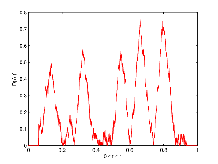
From the other hand, note that $(D(A,k))_{A\leq k\leq N-A}$ is a sequence of centered r.v., except in the vicinity of a change point $\tau_{k}$. In this case, there appears a "hat-function" of size $\delta_{k}:=\big(\mu_{k+1}-\mu_{k}\big)$ approximatively located between $\tau_{k}-A$ and $\tau_{k}+A$, see [5]. Nevertheless, this sequence presents also hats at points different from $(\tau_{1},\ldots,\tau_{K})$, see Figure 2 below. There are false alarms.

In order to eliminate these false alarms, we propose to calculate the p-values $\alpha_{k}$ associated to all detected change points $\big(\tilde{\tau}_{k}\big)_{1\leq k\leq Kmax}$. Then, we keep only the point corresponding to a p-value lesser than a critical level $\alpha_{critic}$. For all $k\in[1,Kmax]$, the p-values are calculated by using the formula $\alpha_{k}=\phi\left(\frac{1}{\overline{\sigma}_{k}}\sqrt{\frac{A_{k}}{2}}|D(A_{k},\tilde{\tau}_{k})|\right)$ where $A_{k}$ is an adaptive window chosen as the minimum of the distances between $\tilde{\tau}_{k}$ and these two neighbors $\tilde{\tau}_{k-1}$ and $\tilde{\tau}_{k+1}$, that is $\displaystyle A_{k}=|\tilde{\tau}_{k}-\tilde{\tau}_{k-1}|\wedge|\tilde{\tau}_{k+1}-\tilde{\tau}_{k}|$. The function $\phi$ denotes the complementary cumulative distribution function of the normal law and $\overline{\sigma}_{k}$ denotes the empirical variance of $X$ on the box $(\tilde{\tau}_{k-1},\tilde{\tau}_{k+1})$.

Remark that $K_{max}$ is an integer fixed by the user. It represents the maximal number of change points. As soon as possible, $K_{max}$ should be chosen bigger than the true number of change points $K$. By convention, one sets $\tau_{0}=\tilde{\tau}_{0}=0$ and $\tau_{K+1}=\tilde{\tau}_{Kmax+1}=N$.

So, the novelty of this work consists in discriminating between true and false alarms by attributing a p-value to each detected change point. By keeping the change points with a p-value smaller than $\alpha_{critic}$, one obtains the same precision as Lavielle & Teyssière (2006) or Lebarbier (2005).
Also, the main advantage of this method lies in its memory and time complexity in $O(N)$.

At first, we give an example on one sample. In the next subsection, this example is plainly confirmed by Monte-Carlo simulations. To begin with, for $N=5000$ we have simulated one replication of a sequence of Gaussian random variable $X_{1},\ldots,X_{N}$ with variance $\sigma^{2}=1$ and mean $\mu(i)=g(i/N)$ where $g$ is a piecewise-constant function with five change points such as $\delta_{k}\in[0.5,1.25]$, see Figure 1 below.

On this sample, we have computed the function $k\mapsto|D(A,k)|$ with $A=300$, see Figure 2.

Both estimators penalized least square criterion (PLSC) and filtered derivative with p-value $\alpha_{critic}=10^{-4}$ provide good results, see Figure 3 and the Monte-Carlo simulation below.

In this subsection, we have made $M=1000$ simulations of independent copies of sequences of Gaussian r.v. $X_{0}^{(k)},\ldots,X_{N}^{(k)}$ with variance $\sigma^{2}=1$ and mean $\mu(i)=g(i/N)$, for $k=1,\dots,M$. On each sample, we apply the FDp-V method and the PLSC method. We find the good number of changes in $98.1\%$ of all cases for the first method and in $97.9\%$ for the second one.

On the one hand, both methods have the same accuracy in terms of percentage of selection of the exact model, Square Error on the configuration of change points or MISE. On the other hand, the filtered derivative with p-value is less expensive in terms of time complexity and memory complexity. Indeed, algorithm based on Minimization of penalized least square criterion can use $39\%$ of computer memory, while Filtered derivative method only needs $0.008\%$. This plainly confirms the difference of time and memory complexity, i.e. $O(N^{2})$ versus $O(N)$.

Observe that algorithms based on penalized least square are considered by Davis et al. (2008) as maximizing a posteriori (MAP) criterion, whereas filtered derivative is based on sliding window and could be adapted to sequential detection, see for instance Bertrand (2000) and Bertrand & Fleury (2008).

Let $X$ be a Gaussian centered process with stationary increments, it is known, see Cramér & Leadbetter (1967), that this process has the harmonizable representation $X(t)=\int_{I\!\!R}\big(e^{it\xi}-1\big)f^{1/2}(\xi)dW(\xi)$ for all $t\in I\!\!R$ where $W(dx)$ is a complex Brownian measure such that $X(t)$ is a real number for all $t\in I\!\!R$. This process has long memory, but its wavelet coefficient $d_{\psi}(a,b)$ is a short memory Gaussian process where, for a scale and a shift $(a,b)\in I\!\!R_{+}^{*}\times I\!\!R$ and a wavelet $\psi$ with a compact time support $[L_{1},L_{2}]$, one has defined

Moreover, for any fixed scale $a$, $\displaystyle b\mapsto d_{\psi}(a,b)$ is a stationary, centered, Gaussian process with variance $\;\displaystyle\mathcal{I}_{\psi}(a):=\int_{I\!\!R}|\widehat{\psi}(x)|^{2}\,f(x/a)\,dx$, see Bardet & Bertrand (2007). Next, we assume that the signal is a Gaussian process, centered, with locally stationary increments given by the representation formula

where $\xi\mapsto f(t,\xi)$ is an even and positive function, called spectral density piecewise constant, i.e., there exists a partition $\tau_{1}<\tau_{2}<\dots<\tau_{K}$ and Hurst parameters $H=(H_{0},H_{1},\ldots,H_{K})$ such that $f(t,\xi)=f_{k}(\xi)=C(H_{k})|\xi|^{-2H_{k}-1}$ for $t\in[\tau_{k},\tau_{k+1}[$ and $C(H_{k})=\pi^{-1}H_{k}\Gamma(2H_{k})\sin(\pi H_{k})$. Thus the series $\log|d_{\psi}(a,b_{i})|^{2}$ where $d_{\psi}(a,b)$ is defined by (1) and $b_{i}=i\in I\!\!N$ has a piecewise constant mean $\mu_{i}$ and a finite known variance, more precisely, one has $\,\displaystyle\log|d_{\psi}(a,b_{i})|^{2}=\mu_{i}+\zeta_{i}\,$ where $\zeta_{i}$ are weakly dependent r.v. of law $\ln|U|^{2}$ with $U\sim\mathcal{N}(0,1)$ and $\,\displaystyle\mu_{i}=\ln\int_{I\!\!R}|\widehat{\psi}(x)|^{2}\,f_{k}(x/a)\,dx\;$ if $b_{i}\in[\tau_{k}-aL_{1},\tau_{k+1}-aL_{2}]$.

First, for $T=10^{5}$, we have simulated one realization of process $(X(t))_{t\in[0,T]}$ with five change points $\textbf{$\tau$}=\{12500,25496,43045,70083,82040\}$ and Hurst parameters $H=(0.55,0.67,0.53,0.61,0.7,0.57)$. Let us stress that, after having changed the scale in order to obtain Hurst index belonging to $(0,1)$, the configuration of change points and means is the same as in Section 1.

Next, for a frequency $1/a=0.2$Hz and by using the Daubechies wavelet of order 6, we have calculated the wavelet coefficients $(d_{\psi}(a,b_{0}),\ldots,d_{\psi}(a,b_{N}))$ with $b_{k}=k$. Figure 5 below displays the sequence $(Y_{0},\ldots,Y_{N})$ where $Y_{k}=\log|d_{\psi}(a,b_{k})|^{2}$. Then, we have calibrated the Filtered derivative algorithm with $A=500$ and $\alpha_{critic}=10^{-11}$. We observe that the detected change points perfectly fit the theoretical configuration of changes.

Note that we can not use penalized least square criterion due to the size of data, indeed PLSC would have need $80$GB which is almost $150$ times our computer memory capacity.

References

- [1] Antoch, J. & Hušková, M. (1994), Procedures for the detection of multiple changes in series of independent observations, in Proc. of the 5th Prague Symposium on Asymptotic Statistics, Physica Verlag, 3–20.
- [2] Bai J. and Perron P. (1998). Estimating and testing linear models with multiple structural changes. Econometrica 66, p. 47-78.
- [3] Bardet, J.M. & Bertrand, P.R. (2007). Identification of the multiscale fractional Brownian motion with biomechanical applications. J. of Time Series. Anal. 28, 1–52.
- [4] M. Basseville & I. Nikiforov, (1993). Detection of Abrupt Changes: Theory and Application. Prentice Hall, Englewood Cliffs, NJ.
- [5] Bertrand, P. R. (2000). A local method for estimating change points: the hat-function. Statistics 34, 215–235.
- [6] Bertrand, P. R. and Fleury, G. (2008). Detecting Small Shift on the Mean by Finite Moving Average, International Journal of Statistics and Management System, vol. 3, No 1-2, pp.56-73
- [7] Birgé L. & Massart, P. (2007). Minimal penalties for Gaussian model selection. Probab. Theory Related Fields 138, 33–73.
- [8] Cramér, H. & Leadbetter, M. R. (1967). Stationary and related stochastic processes. Sample function properties and their applications. Wiley and Sons.
- [9] Csörgo, M.; Horváth, L.; Limit Theorem in Change-Point Analysis, Wiley, (1997).
- [10] Davis, R. A.; Lee, T. C. M.; Rodriguez-Yam, G. A. (2006). Structural break estimation for nonstationary time series models. J. Amer. Statist. Assoc. 101, no. 473, 223–239.
- [11] Lavielle, M. & Moulines, E. (2000). Least-squares estimation of an unknown number of shifts in a time series. J. of Time Series Anal. 21, 33–59.
- [12] Lavielle, M. & Teyssière, G. (2006). Detection of multiple change points in multivariate time series. Lithuanian Math. J. 46, 287–306.
- [13] Lebarbier, E. (2005). Detecting multiple change-points in the mean of Gaussian process by model selection. Signal Processing 85, 717–736.
- [14] Task force of the European Soc. Cardiology and the North American Society of Pacing and Electrophysiology (1996). Heart rate variability. Standards of measurement, physiological interpretation, and clinical use. Circulation 93, 1043–1065.