\history

Received on *****; revised on *****; accepted on ***** \editorAssociate Editor: *****

RNA-RNA interaction prediction based on multiple sequence alignments

Andrew X. Li ¹ Manja Marz ² Jing Qin ³ Christian M. Reidys ^1,4 Note: to whom correspondence should be addressed. Phone: *86-22-2350-6800; Fax: *86-22-2350-9272; duck@santafe.edu Address: ¹Center for Combinatorics, LPMC-TJKLC, Nankai University Tianjin 300071, P.R. China
² RNA Bioinformatics Group, Philipps-University Marburg, Marbacher Weg 6, 34037 Marburg, Germany
³Max Planck Institute for Mathematics in the Sciences, Inselstrasse 22, D-04103 Leipzig, Germany
⁴College of Life Science, Nankai University Tianjin 300071, P.R. China.

Abstract

1 Motivation

Many computerized methods for RNA-RNA interaction structure prediction have been developed. Recently, $O(N^{6})$ time and $O(N^{4})$ space dynamic programming algorithms have become available that compute the partition function of RNA-RNA interaction complexes. However, few of these methods incorporate the knowledge concerning related sequences, thus relevant evolutionary information is often neglected from the structure determination. Therefore, it is of considerable practical interest to introduce a method taking into consideration both thermodynamic stability and sequence covariation.

2 Results

We present the a priori folding algorithm ripalign, whose input consists of two (given) multiple sequence alignments (MSA). ripalign outputs (1) the partition function, (2) base-pairing probabilities, (3) hybrid probabilities and (4) a set of Boltzmann-sampled suboptimal structures consisting of canonical joint structures that are compatible to the alignments. Compared to the single sequence-pair folding algorithm rip, ripalign requires negligible additional memory resource. Furthermore, we incorporate possible structure constraints as input parameters into our algorithm.

3 Availability

The algorithm described here is implemented in C as part of the rip package. The supplemental material, source code and input/output files can freely be downloaded from http://www.combinatorics.cn/cbpc/ripalign.html.

4 Contact

Christian Reidys duck@santafe.edu

^†^†firstpage: 1

Keywords multiple sequence alignment, RNA-RNA interaction, joint structure, dynamic programming, partition function, base pairing probability, hybrid, loop, RNA secondary structure.

5 Introduction

RNA-RNA interactions play a major role at many different levels of the cellular metabolism such as plasmid replication control, viral encapsidation, or transcriptional and translational regulation. With the discovery that a large number of transcripts in higher eukaryotes are noncoding RNAs, RNA-RNA interactions in cellular metabolism are gaining in prominence. Typical examples of interactions involving two RNA molecules are snRNAs (Forne et al., 1996); snoRNAs with their targets (Bachellerie et al., 2002); micro-RNAs from the RNAi pathway with their mRNA target (Ambros, 2004; Murchison and Hannon, 2004); sRNAs from Escherichia coli (Hershberg et al., 2003; Repoila et al., 2003); and sRNA loop-loop interactions (Brunel et al., 2003). The common feature in many ncRNA classes, especially prokaryotic small RNAs, is the formation of RNA-RNA interaction structures that are much more complex than the simple sense-antisense interactions.

As it is the case for the general RNA folding problem with unrestricted pseudoknots (Akutsu, 2000), the RNA-RNA interaction problem (RIP) is NP-complete in its most general form (Alkan et al., 2006; Mneimneh, 2009). However, polynomial-time algorithms can be derived by restricting the space of allowed configurations in ways that are similar to pseudoknot folding algorithms (Rivas and Eddy, 1999). The simplest approach concatenates the two interacting sequences and subsequently employs a slightly modified standard secondary structure folding algorithm. The algorithms RNAcofold (Hofacker et al., 1994; Bernhart et al., 2006), pairfold (Andronescu et al., 2005), and NUPACK (Ren et al., 2005) subscribe to this strategy. A major shortcoming of this approach is that it cannot predict important motifs such as kissing-hairpin loops. The paradigm of concatenation has also been generalized to the pseudoknot folding algorithm of Rivas and Eddy (1999). The resulting model, however, still does not generate all relevant interaction structures (Chitsaz et al., 2009b). An alternative line of thought is to neglect all internal base-pairings in either strand and to compute the minimum free energy (MFE) secondary structure for their hybridization under this constraint. For instance, RNAduplex and RNAhybrid (Rehmsmeier et al., 2004) follows this line of thought. RNAup (Mückstein et al., 2006; Mückstein et al., 2008) and intaRNA (Busch et al., 2008) restrict interactions to a single interval that remains unpaired in the secondary structure for each partner. These models have proved particularly useful for bacterial sRNA/mRNA interactions (Geissmann and Touati, 2004).

Pervouchine (2004) and Alkan et al. (2006) independently proposed MFE folding algorithms for predicting the joint structure of two interacting RNA molecules with polynomial time complexity. In their model, a “joint structure” means that the intramolecular structures of each molecule are pseudoknot-free, the intermolecular binding pairs are noncrossing and there exist no so-called “zig-zags”, see supplement material (SM) for detailed definition. The optimal joint structure is computed in $O(N^{6})$ time and $O(N^{4})$ space via a dynamic programming (DP) routine.

A more reliable approach is to consider the partition function, which by construction integrates over the Boltzmann-weighted probability space, allowing for the derivation of thermodynamic quantities, like e.g. equilibrium concentration, melting temperature and base-pairing probabilities. The partition function of joint structures was independently derived by Chitsaz et al. (2009b) and Huang et al. (2009) while the base-pairing probabilities are due to Huang et al. (2009).

A key quantity here is the probability of hybrids, which cannot be recovered from base pairing probabilities since the latter can be highly correlated. Huang et al. (2010) presented a new hybrid-based decomposition grammar, facilitating the computation of the nontrivial hybrid-probabilities as well as the Boltzmann sampling of RNA-RNA interaction structures. The partition function of joint structures can be computed in $O(N^{6})$ time and $O(N^{4})$ space and current implementations require very large computational resources. Salari et al. (2009) recently achieved a substantial speed-up making use of the observation that the external interactions mostly occur between pairs of unpaired regions of single structures. Chitsaz et al. (2009a) introduced tree-structured Markov Random Fields to approximate the joint probability distribution of multiple $(\geq 3)$ contact regions.

Unfortunately, incompleteness of the underlying energy model, in particular for hybrid- and kissing-loops, may result in prediction inaccuracy. One way of improving this situation is to involve phylogenetic information of multiple sequence alignments (MSA).

In an MSA homologous nucleotides are grouped in columns, where homologous is interpreted in both: structural as well as evolutionary sense. I.e. a column of nucleotides occupies similar structural positions and all diverge from a common ancestral nucleotide. Also, many ncRNAs show clear signs of undergoing compensatory mutations along evolutionary trajectories. In conclusion, it seems reasonable to stipulate that a non-negligible part of the existing RNA-RNA interactions contain preserved but covarying patterns of the interactions (Seemann et al., 2010). Therefore we can associate a consensus interaction structure to pairs of interacting MSAs (see Section 6.1).

Along these lines Seemann et al. (2010) presented an algorithm PETcofold for prediction of RNA-RNA interactions including pseudoknots in given MSAs. Their algorithm is an extension of PETfold (Seemann et al., 2008) using elements of RNAcofold (Bernhart et al., 2006) and computational strategies for hierarchical folding (Gaspin and Westhof, 1995; Jabbari et al., 2007). However, PETcofold is an approximation algorithm and further differences between the two approaches will be discussed in Section .

Here, we present the algorithm ripalign which computes the partition function, base-pairing as well as hybrid probabilities and performs Boltzmann-sampling on the level of MSAs. ripalign represents a generalization of rip to pairs of interacting MSAs and a new grammar of canonical interaction structures. The latter is of relevance since there are no isolated base pairs in molecular complexes.

One important step consists in identifying the notion of a joint structure compatible to a pair of interacting MSAs. Our notion is based on the framework of Hofacker et al. (2002), where a sophisticated cost function capturing thermodynamic stability as well as sequence covariation is employed. Furthermore ripalign is tailored to take structure constraints, such as blocked nucleotides known e.g. from chemical probing, into account.

{methods}

6 Theory

6.1 Multiple sequence alignments and compatibility

A MSA, $\bar{\mathbf{R}}$ , consists of $m_{\bar{\mathbf{R}}}$ RNA sequences of known species. Denoting the length of the aligned sequences by $N$ , $\bar{\mathbf{R}}$ constitutes a $m_{\bar{\mathbf{R}}}\times N$ matrix, having $5^{\prime}-3^{\prime}$ oriented rows, $\bar{\mathbf{R}}^{i}$ and columns, ${\bar{\mathbf{R}}}_{i}$ . Its $(i,j)$ -th entry, $\bar{\mathbf{R}}^{i}_{j}$ , is a nucleotide, $\textbf{A},\textbf{U},\textbf{G},\textbf{C}$ or a gap denoted by ..

For any pair $(\bar{\mathbf{R}},\bar{\mathbf{S}})$ we assume that $\bar{\mathbf{S}}$ is a $m_{\bar{\mathbf{S}}}\times M$ matrix, whose rows carry $3^{\prime}-5^{\prime}$ orientation.

In the following we shall assume that a pair of RNA sequences can only interact if they belong to the same species. A pair $(\bar{\mathbf{R}},\bar{\mathbf{S}})$ , can interact if for any row $\bar{\mathbf{R}}^{i}$ , there exist at least one row in $\bar{\mathbf{S}}$ that can interact with $\bar{\mathbf{R}}^{i}$ .

Given a pair of interacting MSAs $(\bar{\mathbf{R}},\bar{\mathbf{S}})$ , let $m$ be the total number of potentially interacting pairs. ripalign exhibits a pre-processing step which generates a $m\times N$ -matrix $\mathbf{R}$ and a $m\times M$ -matrix $\mathbf{S}$ such that $(\mathbf{R}^{i},\mathbf{S}^{i})$ range over all $m$ potentially interacting RNA-pairs, see Tab. 1 and the SM, Section 1.2.

sp.	$\bar{\mathbf{R}}$	sp.	$\bar{\mathbf{S}}$	sp.	$\mathbf{R}$	$\mathbf{S}$
$\theta_{1}$	AGAACGGA	$\theta_{1}$	GGGCCG	$\theta_{1}$	AGAACGGA	GGGCCG
$\theta_{1}$	GAAACGGA	$\theta_{1}$	AGUUAG	$\theta_{1}$	AGAACGGA	AGUUAG
$\theta_{2}$	AGA.CGAC	$\theta_{2}$	AGGCAG	$\theta_{1}$	GAAACGGA	GGGCCG
		$\theta_{2}$	..GUGG	$\theta_{1}$	GAAACGGA	AGUUAG
				$\theta_{2}$	AGA.CGAC	AGGCAG
				$\theta_{2}$	AGA.CGAC	..GUGG

Table 1: Preprocessing in ripalign: Given a pair of MSAs

(\bar{\mathbf{R}},\bar{\mathbf{S}})

, where

\bar{\mathbf{R}}

consists of three aligned RNA sequences of species (sp.)

\theta_{1}

\theta_{2}

\bar{\mathbf{S}}

in turn consists of four aligned sequences of species

\theta_{1}

and

\theta_{2}

. Then we obtain the matrix-pair

({\mathbf{R}},{\mathbf{S}})

, where

(\mathbf{R}^{i},\mathbf{S}^{i})

1\leq i\leq 6

, ranges over all the six potentially interacting RNA-pairs.

We shall refer in the following to $\mathbf{R}$ and $\mathbf{S}$ as MSAs ignoring the fact that they have multiple sequences.

We proceed by defining joint structures that are compatible to a fixed $({\mathbf{R}},{\mathbf{S}})$ . To this end, let us briefly review some concepts introduced in Huang et al. (2009).

A joint structure $J(R,S,I)$ is a graph consisting of
(j1) Two secondary structures $R$ and $S$ , whose backbones are drawn as horizontal lines on top of each other and whose arcs are drawn in the upper and lower halfplane, respectively. We consider $R$ over a $5^{\prime}$ to $3^{\prime}$ oriented backbone $(R_{1},\dots,R_{N})$ and $S$ over a $3^{\prime}$ to $5^{\prime}$ oriented backbone $(S_{1},\dots,S_{M})$ and refer to any $R$ - and $S$ -arcs as interior arcs.
(j2) An additional set $I$ , of noncrossing arcs of the form $R_{i}S_{j}$ (exterior arc), where $R_{i}$ and $S_{j}$ are unpaired in $R$ and $S$ .
(j3) $J(R,S,I)$ contains no “zig-zags” (see SM).

The subgraph of a joint structure $J(R,S,I)$ induced by a pair of subsequences $(R_{i},R_{i+1},\dots,R_{j})$ and $(S_{h},S_{h+1},\dots,S_{\ell})$ is denoted by $J_{i,j;h,\ell}$ . In particular, $J(R,S,I)=J_{1,N;1,M}$ and $J_{i,j;h,\ell}\subset J_{a,b;c,d}$ if and only if $J_{i,j;h,\ell}$ is a subgraph of $J_{a,b;c,d}$ induced by $(R_{i},\dots,R_{j})$ and $(S_{h},\dots,S_{\ell})$ . In particular, we use $S[i,j]$ to denote the subgraph of $J_{1,N;1,M}$ induced by $(S_{i},S_{i+1},\dots,S_{j})$ , where $S[i,i]=S_{i}$ and $S[i,i-1]=\varnothing$ .

Given a joint structure, $J_{a,b;c,d}$ , a tight structure (TS), $J_{i,j;h,\ell}$ , (Huang et al., 2009) is a specific subgraph of $J_{a,b;c,d}$ indexed by its type $\in\{\circ,\bigtriangledown,\square,\bigtriangleup\}$ , see Fig. 1. For instance, we use $J^{\square}_{i,j;h,\ell}$ to denote a TS of type $\square$ .

Refer to caption — Figure 1: The four basic types of tight structures are given as follows: $\circ:$ $\{R_{i}S_{h}\}=J_{i,j;h,\ell}$ and $i=j$ , $h=\ell$ ; $\bigtriangledown:$ $R_{i}R_{j}\in J_{i,j;h,\ell}$ and $S_{h}S_{\ell}\not\in J_{i,j;h,\ell}$ ; $\square:$ $\{R_{i}R_{j},S_{h}S_{\ell}\}\in J_{i,j;h,\ell}$ ; $\bigtriangleup:$ $S_{h}S_{\ell}\in J_{i,j;h,\ell}$ and $R_{i}R_{j}\not\in J_{i,j;h,\ell}$ .

A hybrid is a joint structure $J^{\mathsf{Hy}}_{i_{1},i_{\ell};j_{1},j_{\ell}}$ , i.e. a maximal sequence of intermolecular interior loops consisting of a set of exterior arcs $(R_{i_{1}}S_{j_{1}},\dots,R_{i_{\ell}}S_{j_{\ell}})$ where $R_{i_{h}}S_{j_{h}}$ is nested within $R_{i_{h+1}}S_{j_{h+1}}$ and where the internal segments $R[i_{h}+1,i_{h+1}-1]$ and $S[j_{h}+1,j_{h+1}-1]$ consist of single-stranded nucleotides only. That is, a hybrid is the maximal unbranched stem-loop formed by external arcs.

A joint structure $J(R,S,I)$ is called canonical if and only if:
(c1) each stack in the secondary structures $R$ and $S$ is of size at least two, i.e. there exist no isolated interior arcs,
(c2) each hybrid contains at least two exterior arcs.
In the following, we always assume a joint structure to be canonical.

Next, we come to $(\mathbf{R},\mathbf{S})$ -compatible joint structures. In difference to single sequence compatibility, this notion involves statistical information of the MSAs.

The key point consists in specifying under which conditions two vertices contained in $(R_{1},\dots,R_{N},S_{1},\dots,S_{M})$ can pair. This is obtained by a generalization of the RNAalifold approach (Hofacker et al., 2002). We specify these conditions for interior $(c_{i,j}^{\mathbf{R}})$ , $(c_{i,j}^{\mathbf{S}})$ and exterior pairs $(c_{i,j}^{\mathbf{R,S}})$ in eq. (6.3)-(6.5).
For interior arcs $(R_{i},R_{j})$ , let $\text{X,Y}\in\{\textbf{A},\textbf{U},\textbf{G},\textbf{C}\}$ . Let $f_{ij}^{\mathbf{R}}(\text{XY})$ be the frequency of $(\text{X},\text{Y})$ which exists in the $2$ -column sub-matrix $(\mathbf{R}_{i},\mathbf{R}_{j})$ as a row-vector and

C_{i,j}^{\mathbf{R}}=\sum_{\text{XY},\text{X}^{\prime}\text{Y}^{\prime}}f_{ij}^{\mathbf{R}}(\text{XY})D^{\mathbf{R}}_{\text{XY},\text{X}^{\prime}\text{Y}^{\prime}}f^{\mathbf{R}}_{ij}(\text{X}^{\prime}\text{Y}^{\prime}).

(6.1)

Here XY and X^′Y^′ independently range over all 16 elements of $\{\textbf{A},\textbf{U},\textbf{G},\textbf{C}\}\times\{\textbf{A},\textbf{U},\textbf{G},\textbf{C}\}$ and $D^{\mathbf{R}}_{\text{XY},\text{X}^{\prime}\text{Y}^{\prime}}=d_{H}(\text{XY},\text{X}^{\prime}\text{Y}^{\prime})$ , i.e. the Hamming distance between XY and X^′Y^′ in case of XY and X^′Y^′ being Watson-Crick, or GU wobble base pair and 0, otherwise. Furthermore, we introduce $q_{i,j}^{\mathbf{R}}$ to deal with the inconsistent sequences

q_{i,j}^{\mathbf{R}}=1-\frac{1}{m}\sum_{h}\{\Pi_{i,j}^{h}(\mathbf{R})+\delta(\mathbf{R}_{i}^{h},\text{gap})\delta(\mathbf{R}_{j}^{h},\text{gap})\},

(6.2)

where $\delta(x,y)$ is the Kronecker delta and $\Pi_{i,j}^{h}(\mathbf{R})$ is equal to 1 if $\mathbf{R}^{h}_{i}$ and $\mathbf{R}^{h}_{j}$ are Watson-Crick or GU wobble base pair and 0, otherwise. Now we obtain $B_{i,j}^{\mathbf{R}}=C_{i,j}^{\mathbf{R}}-\phi_{1}q_{i,j}^{\mathbf{R}}$ . Based on sequence data, the threshold for pairing $B^{\mathbf{R}}_{*}$ as well as the weight of inconsistent sequences $\phi_{1}$ are computed we have

(c_{i,j}^{\mathbf{R}})\quad B^{\mathbf{R}}_{i,j}\geq B^{\mathbf{R}}_{*}

(6.3)

The case of two positions $S_{i}$ and $S_{j}$ is completely analogous

(c_{i,j}^{\mathbf{S}})\quad B^{\mathbf{S}}_{i,j}\geq B^{\mathbf{S}}_{*},

(6.4)

where $B^{\mathbf{S}}_{i,j}$ and $B^{\mathbf{S}}_{*}$ are analogously defined.

As for $(c_{i,j}^{\mathbf{R},\mathbf{S}})$ a further observation factors in: since many ncRNA show clear signs of undergoing compensatory mutations in the course of evolution (Seemann et al., 2010; Marz et al., 2008), we postulate the existence of a non-negligible amount of RNA-RNA interactions containing conserved pairs, consistent mutations, compensatory mutations as well as inconsistent mutations. Based on this observation we arrive at

(c_{i,j}^{\mathbf{R},\mathbf{S}})\quad B^{\mathbf{R},\mathbf{S}}_{i,j}\geq B^{\mathbf{R},\mathbf{S}}_{*},

(6.5)

where $B^{\mathbf{R},\mathbf{S}}_{i,j}$ and $B^{\mathbf{R},\mathbf{S}}_{*}$ are analogously defined as the case for $B^{\mathbf{R}}_{i,j}$ and $B^{\mathbf{R}}_{*}$ .

A joint structure $J$ is compatible to $(\mathbf{R},\mathbf{S})$ if for any $J$ -arc, the corresponding intra- or inter-positions can according to eq. (6.3)-(6.5) pair.

6.2 Energy model

According to Huang et al. (2009) joint structures can be decomposed into disjoint loops. These loop-types include standard hairpin-, bulge-, interior- and multi-loops found in RNA secondary structures as well as hybrid and kissing-loops. Following the energy parameter rules of Mathews et al. (1999), the energy of each loop can be obtained as a sum of the energies associated with non-terminal symbols, i.e. graph properties (sequence independent) and an additional contributions which depend uniquely on the terminal bases (sequence dependent).

Suppose we are given a joint structure $J$ , compatible to a pair $\mathcal{P}=(\mathbf{R},\mathbf{S})$ . Let $L\in J$ be a loop and let $\mathcal{F}_{L,i}$ represent the loop energy of the $i$ -th interaction-pair $(\mathbf{R}^{i},\mathbf{S}^{i})$ . Then the loop energy of $\mathcal{P}$ is

\mathcal{F}_{L,\mathcal{P}}=1/m\sum_{i}\mathcal{F}_{L,i}.

(6.6)

We consider the energy of the structure as the sum of all loop contributions:

\mathcal{F}_{J}=\sum_{L\in J}\mathcal{F}_{L,\mathcal{P}}.

(6.7)

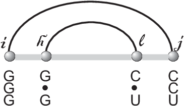
To save computational resources, gaps are treated as bases in ripalign. Thus only alignment positions contribute as indices and loop sizes. Since no measured energy parameters for nonstandard base-pairs are available at present time, additional terminal-dependent contributions for the latter are ignored. For instance, let ${\sf Int}_{i,j;h,l}$ denote an interior loop formed by $R_{i}R_{j}$ and $R_{h}R_{\ell}$ and $\mathcal{F}_{\textsf{Int},\mathcal{P}}^{i,j;h,\ell}$ denote the free energy of $\textsf{Int}_{i,j;h,l}$ with respect to the aligned sequences in $\mathcal{P}$ . Then $\mathcal{F}_{\textsf{Int},\mathcal{P}}^{i,j;h,\ell}$ associated to the three aligned subsequences of Fig. 2 reads

\mathcal{F}^{\textsf{Int},\mathcal{P}}_{i,j;h,\ell}=\frac{1}{3}(3G^{\sf Int}_{i,j;h,\ell}+G_{*,\textbf{G,C;G,C}}^{\sf Int}+G_{*,\textbf{G,U;G,U}}^{\sf Int}+G_{*,\textbf{G,C;gap,gap}}^{\sf Int}).

(6.8)

Here $G^{\sf Int}_{i,j;h,\ell}$ represents contributions related exclusively to the positions of the interior loop while $G^{\sf Int}_{*,\textbf{A,B;C,D}}$ represents additional contributions related to the specific nucleotides which form the interior loop. We set $G_{*,\textbf{G,C;gap,gap}}^{\sf Int}$ to be zero.

6.3 The grammar of canonical joint structures and the partition function

The partition function algorithm is easily extended to work with the modified energy functions given in eq. (6.7). The reformulation of the original hybrid-grammar into a grammar of canonical joint structures represents already for single interaction pairs a significant improvement in prediction quality. The original rip-grammar would oftentimes encounter joint structures having a hybrid composed by a single isolated exterior arc, see Fig. 8.
In order to decompose canonical joint structures via the unambiguous grammar introduced in Section 6.3, we distinguish the two types (Type cc and Type c) of TS’s of type $\bigtriangledown$ , $\bigtriangleup$ or $\square$ . Given a TS of type $\bigtriangledown$ , denoted by $J^{\bigtriangledown}_{i,j;h,\ell}$ , we write depending on whether $R_{i+1}R_{j-1}\in J^{\bigtriangledown}_{i,j;h,\ell}$ , $J^{\bigtriangledown,cc}_{i,j;h,\ell}$ and $J^{\bigtriangledown,c}_{i,j;h,\ell}$ , respectively. Analogously, we define $J^{\square,cc}_{i,j;h,\ell}$ , $J^{\square,c}_{i,j;h,\ell}$ and $J^{\bigtriangleup,cc}_{i,j;h,\ell}$ , $J^{\bigtriangleup,c}_{i,j;h,\ell}$ , see Fig. 3.
Fig. 4 summarizes the two basic steps of the canonical-grammar: (I) interior arc-removal to reduce TS, and (II) block-decomposition to split a joint structure into two smaller blocks. The key feature here is, that since $J$ is canonical, the smaller blocks are still canonical after block-decomposition. Each decomposition step displayed in Fig. 4 results in substructures which eventually break down into generalized loops whose energies can be directly computed. More details of the decomposition procedures are described in Section 2 of the SM, where we prove that for any canonical joint structure $J$ , there exists a unique decomposition-tree (parse-tree), denoted by $T_{J}$ , see Fig. 5.

6.4 Probabilities and the Boltzmann Sampling

A dynamic programming scheme for the computation of a partition function implies a corresponding computation of probabilities of specific substructures is obtained “from the outside to the inside” and a stochastic backtracing procedure that can be used to sample from the associated distribution (McCaskill, 1990; Ding and Lawrence, 2003; Huang et al., 2010). We remark that the time complexity does not increase linearly as a function of $m$ (see SM Table. 5).
Along the lines of the design of the Vienna software package (Hofacker et al., 1994), ripalign now offers the following features as optional input parameters:
(1) a position $i$ can be restricted to form an interior or an exterior arc. (denoted by “ $-$ ” and “ ^ ”, respectively);
(2) a position $i$ can be forced to be unpaired (denoted by “x”);
(3) a position $i$ can be restricted to form an (interior or an exterior) arc with some position $j$ (denoted by “ $*$ ”);
(4) a pair of positions $i$ and $j$ can be forced to form an interior or exterior arc (denoted by “ $(\,)$ ” or “ $[\,]$ ”, respectively).
However, the above features are optional. Thus ripalign can deal with both scenarios: the absence of any a priori information and the existence of specific information, e.g the location of the Sm-binding site, see Fig. 8.

7 Results and discussion

In this paper we present an a priori $O(N^{6})$ time and $O(N^{4})$ space dynamic programming algorithm ripalign, whose input consists of a pair of interacting MSAs. ripalign requires only marginally more computational resources but is, without doubt, still computationally costly. Approximation algorithms are much faster, for instance PETcofold (Seemann et al., 2010), having a time complexity of $O(m\,(N+M)^{3}\,n)$ , where $m$ is the number of sequences in MSA, $N$ and $M$ being the sequence lengths of the longer and shorter alignment, respectively, and $n<N/2$ is the number of iterations for the adaption of the threshold value to find likely partial secondary structures. Their basic assumption is that the two secondary structures fold independently and that intra-loop evaluation differences are negligible. The flip-side of reducing the complexity of a folding problem by introducing additional assumptions, is however, the uncertainty of the quality of the solution. Point in case here is that the two secondary structures did not evolve independently, but rather correlated by means of their functional interaction. We remark that ripalign (within its complexity limitations) is capable to describe the space of RNA interaction structures, for instance via Boltzmann sampling, in detail and transparency.
ripalign represents significant improvements in the following aspects:
(a) we incorporate evolutionary factors into the RNA-RNA interaction structure prediction via alignments as input,
(b) we introduce the grammar of canonical joint structures of interacting-alignments,
(c) we a priori factor in structural-constraints, like for instance, knowledge on Sm-binding sites.
Below we shall discuss (a), (b) and (c) in more detail in the context of concrete examples. All the MSAs involving in (a), (b) and (c) are listed in SM, Section 2.

(a): The fhlA/OxyS interaction
The OxyS RNA represses fhlA mRNA translation initiation through base-pairing with two short sequencesArgaman and Altuvia (2000), one of which overlaps the ribosome binding sequence and the other resides further downstream, within the coding region of fhlA. Our algorithm predicts correctly both interaction sites based on MSAs, see Fig. 6. In addition, most predicted stacks in the secondary structures of fhlA and OxyS agree well with the most frequent Bolztmann sampled structure. Two more hybrids, $J^{\sf Hy}_{56,59;41,44}$ and $J^{\sf Hy}_{81,83;48,50}$ are predicted in our output. The two additional contact regions, identified in the partition function, exhibit a significantly lower probability. An additional hairpin over $R[72,89]$ is predicted in fhlA, instead of the unpaired segment occurring in the natural structure, can be understood in the context of minimizing free energy. Comparing the prediction based on the MSAs (Fig. 6, middle) with the one based on the consensus sequence (Fig. 6, bottom), we observe:
(1) the secondary structure of fhlA agrees better with the annotation joint structure (Fig. 6, top),
(2) the leftmost hybrid agrees better with that of the annotated structure.
(3) the binding-site probability (see SM, Section 5, eq. (5.5)) of the leftmost hybrid increases by nearly 40%.
On the flip side, due to the gaps in seven out of eight subsequences induced by $R[98,102]$ (Column 98-102 in fhlA), the prediction quality of the right-most hybrid and its corresponding contact-region probability decreases slightly.
Let us next contrast our results with those of PETcofold, see Fig. 7. The latter predicts one of the two interaction sites. The second site is predicted subject to the condition that constrained stems were not extended (Seemann et al., 2010). It can furthermore be observed that in order to predict the second hybrid, at the same time the secondary structures prediction of both fhlA and OxyS gets worse. ripalign predicts both: the interaction sites situated in fhlA and comes close to predicting the secondary structures of fhlA as well as OxyS without any additional constraints.

(b): The SmY-10/SL-1 interaction of C. elegans
MacMorris et al. (2007) stipulated that SmY-10 RNA, possible involved in trans-splicing, interacts with the splice leader RNA (SL1 RNA). In Fig. 8, we show that the Sm-binding sites (colored in red) of the RNA molecules SmY-10 and SL-1 are $R[56,62]$ and $S[25,31]$ , respectively. In Fig. 8, the top structure is being predicted by rip (Huang et al., 2010). We observe that firstly a stack in SmY-10 consisting of the single arc $R_{24}S_{67}$ and secondly the nucleotides of the Sm-binding sites form intra base pairs. The canonical grammar presented here restricts the configuration ensemble to canonical joint structures, resulting in the structure presented in Fig. 8 (middle) in which the peculiar isolated interaction arc disappears. However, the nucleotides of the Sm-binding sites still form either intra or inter-molecular base pairs. Incorporating the structural constraints option we derive the bottom structure displayed in Fig. 8. Here the Sm-binding sites are single-stranded. In Table. 2 we elaborate this point further and show that the combination of canonical grammar and structural constraints eliminate unwanted hybrids and “free” the nucleotides attributed to Sm-binding sites of unwanted interactions.

	I	II	III
1	$J^{\sf{Hy}}_{37,40;79,82}$	$J^{\sf{Hy}}_{40,41;50,51}$	$J^{\sf{Hy}}_{5,6;9,10}$
2	$J^{\sf{Hy}}_{40,41;50,51}$	$J^{\sf{Hy}}_{39,40;51,52}$	$J^{\sf{Hy}}_{76,78;90,92}$
3	$J^{\sf{Hy}}_{76,78;90,92}$	$J^{\sf{Hy}}_{76,78;90,92}$	$J^{\sf{Hy}}_{37,40;79,82}$
4	$\mathbf{R_{11}S_{10}}$	$J^{\sf{Hy}}_{11,12;9,10}$	$J^{\sf{Hy}}_{78,80;89,91}$
5	$J^{\sf{Hy}}_{16,18;33,35}$	$J^{\sf{Hy}}_{78,80;89,91}$	$J^{\sf{Hy}}_{11,12;51,52}$
6	$J^{\sf{Hy}}_{54,57;65,68}$	$J^{\sf{Hy}}_{54,57;65,68}$	$J^{\sf{Hy}}_{16,17;47,48}$

Table 2: Top 6 probable hybrids predicted by rip and ripalign: Interaction of two specific RNA molecules, SL1 and SmY-10 of Caenorhabditis elegans as illustrated in Fig. 8. The top 6 probable hybrids predicted by rip implemented by Huang et al. (2010) is shown in column I. The hybrids listed in column II are predicted by ripalign without any structure constraint. The hybrids listed in Column III are predicted by ripalign under the structural constraints that

\textbf{5'-AAUUUUUG-3'}(R[56,62])

and

\textbf{3'-GUUUUAA-5'}(S[25,31])

are Sm-binding sites (colored in red) in SmY-10 and SL-1, respectively. Here, we use

J^{\sf{Hy}}_{i,j;h,l}

to denote the hybrid induced by

R[i,j]

and

S[h,l]

(c): The U4/U6 interaction
Two of the snRNAs involved in pre-mRNA splicing, U4 and U6, are known to interact by base pairing (Zucker-Aprison et al., 1988). We divided all known metazoan U4 and U6 snRNAs into three distinct groups and alignments: protostomia without insects, insects and deuterostomia (Marz et al., 2008). Marz et al. (2008) observed that insects behave in their secondary structure different from other protostomes, see Fig. 9. Comparing all the predicted U4/U6 interactions, displayed in Fig. 9, we can conclude:
(1) the secondary partial structures of the U4/U6 complex for all three groups predicted by ripalign agree predominantly with the described secondary structures in metazoans (Thomas et al., 1990; Otake et al., 2002; Shambaugh et al., 1994; López et al., 2008; Shukla et al., 2002), e.g. as depicted in Fig. 9 (top) for C. elegans (Zucker-Aprison et al., 1988).
(2) for all three groups, Stem I and II (Fig. 9, top) are highly conserved. External ascendancies, such as protein interactions may stabilize stem II additionally.
(3) for all three groups, the $5^{\prime}$ hairpin of U4 snRNA seems highly conserved to interact with the U6 snRNA. This RNA feature is not fully understood, since this element is also believed to contain intraloop interactions and may bind to a 15.5kDa protein Vidovic et al. (2000).
(4) for all metazoans, the U6 snRNA shows conserved intramolecular interactions between the $3^{\prime}$ part and the region downstream of the $5^{\prime}$ -hairpin.
(5) for deuterostomes (Fig. 9, bottom), with a contact-region probability of 45.5%), our algorithm identifies a third U4/U6 interaction, Stem III, to be conserved, which agrees with the findings in Jakab et al. (1997); Brow and Vidaver (1995). For protostomes, a similar feature with a contact-region probability of $\leq 10\%$ can also be assumed.
(6) for both: protostomia (without insects) and deuterostomes, the $5^{\prime}$ hairpin of U6 snRNA seems to interact with the U4 $3^{\prime}$ hairpin. However, this observation does not hold for insects, which agrees with a systematically different secondary structure of spliceosomal RNAs in insects (Marz et al., 2008).

We finally remark that the quality of prediction of ripalign depends critically on the quality of the MSAs. This issue of alignment quality is not easily solved: creating an alignment without knowing the structure is unlikely to produce a structural alignment. It might be an option to realign the sequences of an RNA family taking both the predicted secondary structures and predicted joint structure with other RNA families into consideration. Furthermore, ripalign is limited by its a priori output class of joint structures. Thus ripalign cannot identify any joint structures exhibiting pseudoknots. To save computational resources, we stipulate that only alignment positions contribute as indices and loop sizes. The assumption may cause, for instance, the existence of some interior arcs $R_{i}R_{j}$ having arc-length smaller than three. Bernhart et al. (2008) showed that this problem can be improved substantially by introducing a different, more rational handling of alignment gaps, and by replacing the rather simplistic model of covariance scoring with more sophisticated RIBOSUM-like scoring matrices.

{methods}

Acknowledgements. We want to thank Fenix W.D. Huang and Jan Engelhardt for helpful suggestions. We thank Sharon Selzo of the Modular and BICoC Benchmark Center, IBM and Kathy Tzeng of IBM Life Sciences Solutions Enablement. Their support was vital for all computations presented here. We thank Albrecht Bindereif, Elizabeth Chester and Stephen Rader for their U4/U6 analysis. This work was supported by the 973 Project of the Ministry of Science and Technology, the PCSIRT Project of the Ministry of Education, and the National Science Foundation of China to CMR and his lab, grant No. STA 850/7-1 of the Deutsche Forschungsgemeinschaft under the auspices of SPP-1258 “Small Regulatory RNAs in Prokaryotes”, as well as the European Community FP-6 project SYNLET (Contract Number 043312) to Peter F. Stadler and his lab.

References

Akutsu (2000) Akutsu, T. (2000) Dynamic programming algorithms for RNA secondary structure prediction with pseudoknots. Disc. Appl. Math., 104, 45–62.
Alkan et al. (2006) Alkan, C., Karakoc, E., Nadeau, J., Sahinalp, S. and Zhang, K. (2006) RNA-RNA interaction prediction and antisense RNA target search. J. Comput. Biol., 13, 267–282.
Ambros (2004) Ambros, V. (2004) The functions of animal microRNAs. Nature, 431, 350–355.
Andronescu et al. (2005) Andronescu, M., Zhang, Z. C. and Condon, A. (2005) Secondary structure prediction of interacting RNA molecules. J. Mol. Biol., 345, 1101–1112.
Argaman and Altuvia (2000) Argaman, L. and Altuvia, S. (2000) fhlA repression by OxyS RNA: kissing complex formation at two sites results in a stable antisense-target RNA complex. J. Mol. Biol., 300, 1101–1112.
Bachellerie et al. (2002) Bachellerie, J., Cavaille, J. and Huttenhofer, A. (2002) The expanding snoRNA world. Biochimie, 84, 775–779.
Bernhart et al. (2008) Bernhart, S., Hofacker, I., Will, S., Gruber, A. and Stadler, P. (2008) RNAalifold: improved consensus structure prediction for RNA alignments. BMC Bioinformatics, 9, 474–487.
Bernhart et al. (2006) Bernhart, S., Tafer, H., Mückstein, U., Flamm, C., Stadler, P. and Hofacker, I. (2006) Partition function and base pairing probabilities of RNA heterodimers. Algorithms Mol. Biol., 1, 3.
Brow and Vidaver (1995) Brow, D. and Vidaver, R. (1995) An element in human U6 RNA destabilizes the U4/U6 spliceosomal RNA complex. RNA, 1, 122–131.
Brunel et al. (2003) Brunel, C., Marquet, R., Romby, P. and Ehresmann, C. (2003) RNA loop-loop interactions as dynamic functional motifs. Biochimie, 84, 925–944.
Busch et al. (2008) Busch, A., Richter, A. S. and Backofen, R. (2008) IntaRNA: efficient prediction of bacterial sRNA targets incorporating target site accessibility and seed regions. Bioinformatics, 24, 2849–2856.
Chitsaz et al. (2009a) Chitsaz, H., Backofen, R. and Sahinalp, S. C. (2009a) biRNA: Fast RNA-RNA binding sites prediction. In Proceedings of the 9th Workshop on Algorithms in Bioinformatics (WABI), volume 5724 of LNCS, pp. 25–36. Springer, Berlin / Heidelberg.
Chitsaz et al. (2009b) Chitsaz, H., Salari, R., Sahinalp, S. C. and Backofen, R. (2009b) A partition function algorithm for interacting nucleic acid strands. Bioinformatics, 25, i365–i373.
Ding and Lawrence (2003) Ding, Y. and Lawrence, C. E. (2003) A statistical sampling algorithm for RNA secondary structure prediction. Nucleic Acid Res., 31, 7280–7301.
Forne et al. (1996) Forne, T., Labourier, E., Antoine, E., Rossi, F., Gallouzi, I., Cathala, G., Tazi, J. and Brunel, C. (1996) Structural features of U6 snRNA and dynamic interactions with other spliceosomal components leading to pre-mRNA splicing. Biochimie, 78, 434–442.
Gaspin and Westhof (1995) Gaspin, C. and Westhof, E. (1995) An interactive framework for RNA secondary structure prediction with a dynamical treatment of constraints. J. Mol. Biol, 254.
Geissmann and Touati (2004) Geissmann, T. and Touati, D. (2004) Hfq, a new chaperoning role: binding to messenger RNA determines access for small RNA regulator. EMBO J., 23, 396–405.
Hershberg et al. (2003) Hershberg, R., Altuvia, S. and Margalit, H. (2003) A survey of small RNA-encoding genes in Escherichia coli. Nucleic Acids Res., 31, 1813–1820.
Hofacker et al. (2002) Hofacker, I., Fekete, M. and Stadler, P. (2002) Secondary structure prediction for aligned RNA sequences. J. Mol. Biol., 319, 1059–1066.
Hofacker et al. (1994) Hofacker, I. L., Fontana, W., Stadler, P. F., Bonhoeffer, L. S., Tacker, M. and Schuster, P. (1994) Fast folding and comparison of RNA secondary structures. Monatsh. Chem., 125, 167–188.
Huang et al. (2010) Huang, F., Qin, J., Reidys, C. and Stadler, P. (2010) Target prediction and a statistical sampling algorithm for RNA-RNA interaction. Bioinformatics, 26, 175–181.
Huang et al. (2009) Huang, F. W. D., Qin, J., Stadler, P. F. and Reidys, C. M. (2009) Partition function and base pairing probabilities for RNA-RNA interaction prediction. Bioinformatics, 25, 2646–2654.
Jabbari et al. (2007) Jabbari, H., Condon, A., Pop, A., Pop, C. and Zhao, Y. (2007) Hfold:RNA pseudoknotted secondary structure prediction using hierarchial folding. In R., G. (ed.), In algorithms in Bioinformatics, 7th international workshop, WABI 2007. Philadephia, PA, USA.
Jakab et al. (1997) Jakab, G., Mougin, A., Kis, M., Pollák, T., Antal, M., Branlant, C. and Solymosy, F. (1997) Chlamydomonas U2, U4 and U6 snRNAs. An evolutionary conserved putative third interaction between U4 and U6 snrnas which has a counterpart in the U4atac-U6atac snRNA duplex. Biochimie, 79, 387–395.
López et al. (2008) López, M., Rosenblad, M. and Samuelsson, T. (2008) Computational screen for spliceosomal RNA genes aids in defining the phylogenetic distribution of major and minor spliceosomal components. Nucleic Acids Res., 36, 3001–3010.
MacMorris et al. (2007) MacMorris, M., Kumar, M., Lasda, E., Larsen, A., Kraemer, B. and Blumenthal, T. (2007) A novel family of C. elegans snRNPs contains proteins associated with Trans-splicing. RNA, 13, 511–520.
Marz et al. (2008) Marz, M., Kirsten, T. and Stadler, P. F. (2008) Evolution of spliceosomal snRNA genes in metazoan animals. J. Mol. Evol., 67, 594–607.
Mathews et al. (1999) Mathews, D., Sabina, J., Zuker, M. and Turner, D. H. (1999) Expanded sequence dependence of thermodynamic parameters improves prediction of RNA secondary structure. J. Mol. Biol., 288, 911–940.
McCaskill (1990) McCaskill, J. S. (1990) The equilibrium partition function and base pair binding probabilities for RNA secondary structure. Biopolymers, 29, 1105–1119.
Mneimneh (2009) Mneimneh, S. (2009) On the approximation of optimal structures for RNA-RNA interaction. IEEE/ACM Trans. Comp. Biol. Bioinf., 6, 682–688.
Mückstein et al. (2008) Mückstein, U., Tafer, H., Bernhard, S. H., Hernandez-Rosales, M., Vogel, J., Stadler, P. F. and Hofacker, I. L. (2008) Translational control by RNA-RNA interaction: Improved computation of RNA-RNA binding thermodynamics. In Elloumi, M., Küng, J., Linial, M., Murphy, R. F., Schneider, K. and Toma, C. T. (eds.), BioInformatics Research and Development — BIRD 2008, volume 13 of Comm. Comp. Inf. Sci., pp. 114–127. Springer, Berlin.
Mückstein et al. (2006) Mückstein, U., Tafer, H., Hackermüller, J., Bernhard, S. H., Stadler, P. and Hofacker, I. L. (2006) Thermodynamics of RNA-RNA binding. Bioinformatics, 22, 1177–1182.
Murchison and Hannon (2004) Murchison, E. and Hannon, G. (2004) miRNAs on the move: miRNA biogenesis and the RNAi machinery. Curr. Opin. Cell. Biol., 16, 223–229.
Otake et al. (2002) Otake, L., Scamborova, P., Hashimoto, C. and Steitz, J. (2002) The divergent U12-type splicesome is sequired for pre-mRNA splicing and is essential for development in Drosophila. Mol. Cell, 9, 439–446.
Pervouchine (2004) Pervouchine, D. (2004) IRIS: Intermolecular RNA interaction search. Proc. Genome Informatics, 15, 92–101.
Rehmsmeier et al. (2004) Rehmsmeier, M., Steffen, P., Höchsmann, M. and Giegerich, R. (2004) Fast and effective prediction of microRNA/target duplexes. Gene, 10, 1507–1517.
Ren et al. (2005) Ren, J., Rastegari, B., Condon, A. and Hoos, H. H. (2005) Hotknots: heuristic prediction of microRNA secondary structures including pseudoknots. RNA, 11, 1494–1504.
Repoila et al. (2003) Repoila, F., Majdalani, N. and Gottesman, S. (2003) Small non-coding RNAs, co-ordinators of adaptation processes in Escherichia coli: The RpoS paradigm. Mol. Microbiol., 48, 855–861.
Rivas and Eddy (1999) Rivas, E. and Eddy, S. R. (1999) A dynamic programming algorithms for RNA structure prediction including pseudoknots. J. Mol. Biol., 285, 2053–2068.
Salari et al. (2009) Salari, R., Backofen, R. and Sahinalp, S. (2009) Fast prediction of RNA-RNA interaction. In Proceedings of the 9th Workshop on Algorithms in Bioinformatics (WABI), volume 5724 of LNCS, pp. 261–272. Springer, Berlin / Heidelberg.
Seemann et al. (2008) Seemann, S., Gorodkin, J. and Backofen, R. (2008) Unifying evolutionary and thermodynamic information for RNA folding of multiple alignments. Nucleic Acids Res., 36.
Seemann et al. (2010) Seemann, S., Richter, A., Gorodkin, J. and Backofen, R. (2010) Hierarchical folding of multiple sequence alignments for the prediction of structures and RNA-RNA interactions. Algorithms for Molecular Biology, 5. Doi:10.1186/1748-7188-5-22.
Shambaugh et al. (1994) Shambaugh, J., Hannon, G. and Nilsen, T. (1994) The spliceosomal U small nuclear RNAs of Ascaris lumbricoides. Mol. Biochem. Parasitol., 64, 349–352.
Shukla et al. (2002) Shukla, G., Cole, A., Dietrich, R. and Padgett, R. (2002) Domains of human U4atac snRNA required for U12-dependent splicing in vivo. Nucleic Acids Res, 30, 4650–4657.
Thomas et al. (1990) Thomas, J., Lea, K., Zucker-Aprison, E. and Blumenthal, T. (1990) The spliceosomal snRNAs of Caenorhabditis elegans. Nucleic Acids Res., 18, 2633–2642.
Vidovic et al. (2000) Vidovic, I., Nottrott, S., Hartmuth, K., Lührmann, R. and Ficner, R. (2000) Crystal structure of the spliceosomal 15.5kD protein bound to a U4 snRNA fragment. Mol. Cell, 6, 1331–1342.
Zucker-Aprison et al. (1988) Zucker-Aprison, E., Thomas, J. and Blumenthal, T. (1988) C. elegans snRNAs: a model for U4/U6 base pairing. Nucleic Acids Res., 16, 7188–7188.