In contrast with the chaotic advection of perfect tracers, which has been a topic of great interest in the last decades (Arnold [4], Hénon [9], Aref [3], Ottino [13]), little is known about the chaotic motion of inertial particles in laminar flows. Chaotic advection is entirely contained within an elementary equation of kinematics, that is :

$$\frac{d\overrightarrow{X}}{dt}=\overrightarrow{V}_{f}\Big(\overrightarrow{X}(t),t\Big),$$

(1)

where $\overrightarrow{X}(t)$ is the position of a perfect tracer advected by the velocity field $\overrightarrow{V}_{f}$. This velocity field is not required to be turbulent for Lagrangian chaos to take place : it can be laminar and entirely specified. In particular, chaotic advection provides efficient mixing properties, and this is one of the reasons why this effect attracted the attention of the physics community. Mixing is indeed a key phenomenon in nature, and a challenge for engineers as soon as one has to mix large amounts of very viscous fluids, or small quantities of fluid in tiny domains. Nevertheless, the problem “starts rather than ends with the specification of the velocity field” (Ottino [14]), so that many analyses are still being performed to quantify the Lagrangian properties of various flows. Among the mechanisms leading to chaotic advection, the blinking vortex is probably the easiest to perform (Aref [2]). Two key ingredients are required here : the differential rotation and the displacement of the vortex. The former ingredient is responsible for stretching and the latter is required for folding to take place. Many chaotic flows are based on this property and are described in several reviews [3]^, [13].

In the case where the particle is not a pure tracer, surprising chaotic trajectories can also occur, even when the inclusion obeys a linear drag law. For example, aerosols can have complex trajectories in elementary cellular or ABC flows (Maxey & Corrsin [12] ; Wang , Maxey, Burton & Stock [19] ; Mac Laughlin [10] ; Fung [7] ; Tsega, Michaelides & Eschenazi [17] ; Rubin, Jones & Maxey [16]). The complex trajectories reported in these works are due to the non-uniformity of the flow, to the finite response time of the inclusion, and to gravity if any.

The goal of the present work is to show that heavy particles with small response time but non-negligible terminal velocities can have chaotic trajectories under the combined effect of a time-periodic differential rotation (which creates stretching of a particle cloud) and of gravity (which prepares the particle cloud to undergo folding). In particular, we will consider flows where unsteadiness does not suffice to induce Lagrangian chaos, like two-dimensional flows of the form :

$$\overrightarrow{V}_{f}(\overrightarrow{X},t)=\overrightarrow{V}_{f}^{0}(\overrightarrow{X})\,(1+\varepsilon\sin\omega t)$$

(2)

with $\overrightarrow{V}_{f}^{0}(\overrightarrow{X})$ corresponding to a horizontal vortex. Indeed, one can check that the dynamical system (1) is not chaotic in this case, and that fluid points go to and fro along the streamlines of the vortex. Clearly, unsteadiness does not produce chaos because the vortex does not move : not only should we switch the vortex off sometimes, but also should we light it up somewhere else to produce chaos according to the blinking vortex mechanism. However, if gravity is sufficient to displace the particle cloud whilst the vortex is off (or weak), one could expect chaos according to some kind of “gravity-induced blinking vortex”. Note, however, that the key role of gravity in this scenario could also be played by electrostatic forces, or swimming (if particles are bacteria or plankton), to name but a few examples.

The basic vortical flow investigated in this paper is the point vortex :

$$\overrightarrow{V}_{f}^{0}(\overrightarrow{x})=r\Omega(r)\overrightarrow{e}_{\theta},\quad\mbox{with}\quad\Omega(r)=\Omega_{0}(r/R_{0})^{-2}$$

(5)

This velocity field is set non-dimensional in the following by using $R_{0}$ as length units and $1/\Omega_{0}$ as time units. The streamfunction $\psi^{0}$ of this non-dimensional flow therefore reads : $\displaystyle{\psi^{0}(\overrightarrow{X}_{p}(t))=-\frac{1}{2}Log|\overrightarrow{X}_{p}|^{2}.}$ To leading order $O(\varepsilon^{0})$ the particle dynamics reads :

$$\overrightarrow{\dot{X}}_{p}=\overrightarrow{V}_{T}+\overrightarrow{V}_{f}^{0}(\overrightarrow{X}_{p})$$

(6)

and the corresponding trajectories therefore correspond to the iso-values of the hamiltonian :

$$H(x,y)=\psi^{0}(x,y)+xV_{T}$$

and are sketched in figure 1 (b). In order to investigate separatrix splitting under the effect of the $O(\varepsilon^{1})$ terms it is necessary to solve analytically the leading-order motion (6) with $\overrightarrow{X}_{p}(\pm\infty)=A$ (saddle point). To our knowledge, even for the simple flow considered here, this cannot be done. To be precise one cannot obtain a simple solution which would make the Melnikov integral easy to calculate analytically. However, one can obtain semi-analytical results by rescaling the variables. Indeed, we set :

$$\overrightarrow{X}_{p}(t)=\frac{1}{V_{T}}\overrightarrow{Y}(\tau)\quad\mbox{with}\quad\tau=tV_{T}^{2}$$

and notice that the velocity field investigated here satisfies :

$$\overrightarrow{V}_{f}^{0}(\overrightarrow{X}_{p})=V_{T}\overrightarrow{V}_{f}^{0}(\overrightarrow{Y}).$$

The particle dynamics therefore reads :

$$\frac{d\overrightarrow{Y}}{d\tau}=\overrightarrow{V}_{f}^{0}(\overrightarrow{Y})-\overrightarrow{e}_{y}$$

$$+\varepsilon\left[\frac{1}{V_{T}}\overrightarrow{V}_{f}^{1}\left(\frac{1}{V_{T}}\overrightarrow{Y}(\tau),\frac{\tau}{V_{T}^{2}}\right)-kV_{T}^{2}\,\overline{\overline{\nabla}}_{Y}\overrightarrow{V}_{f}^{0}(\overrightarrow{Y}).(\overrightarrow{V}_{f}^{0}(\overrightarrow{Y})-\overrightarrow{e}_{y})\right]$$

(7)

The leading order dynamical equation is now independent of $V_{T}$, and the corresponding phase portrait in the $\overrightarrow{Y}$ plane is similar to the one of figure 1 (b), with the saddle point located at $(1,0)$ (figure 2(a)). Let $\overrightarrow{Y}_{0}(\tau)$ be a solution of the leading-order dynamics :

$$\dot{\overrightarrow{Y}}_{0}=\overrightarrow{V}_{f}^{0}(\overrightarrow{Y}_{0})-\overrightarrow{e}_{y},\quad\overrightarrow{Y}_{0}(\pm\infty)=(1,0)$$

(8)

(the dot upon a $\overrightarrow{Y}$ indicating a derivation with respect to $\tau$) which satisfies, accordingly :

$$\ddot{\overrightarrow{Y}}_{0}=\overline{\overline{\nabla}}_{Y}\overrightarrow{V}_{f}^{0}.(\overrightarrow{V}_{f}^{0}(\overrightarrow{Y}_{0})-\overrightarrow{e}_{y}).$$

When the $O(\varepsilon)$ terms are taken into account, and because the perturbation of the rescaled system is time-periodic (with period $T_{Y}=TV_{T}^{2}$), one usually considers the Poincaré section (or stroboscopic map) $\overrightarrow{Y}(\tau_{0}+nT_{Y})$, with $n=1,2,...$ Because the Poincaré section of the unperturbed system has a hyperbolic point at $(1,0)$, the Poincaré section of the perturbed system will have a hyperbolic point of the same kind (saddle) in the vicinity of $(1,0)$, provided $\varepsilon$ is small enough. An unstable (resp. stable) invariant manifold $W^{u}$ (resp.$W^{s}$ ) will therefore exist in the vicinity of the hyperbolic point. If these two manifolds intersect transversally, they will have an infinity of such intersection points. The non-dissipative (area preserving) character of the $O(\varepsilon^{0})$ system will induce huge stretching, and folding will inevitably follow. The phase portrait in the vicinity of the vortex will take the form sketched in figure 2(b) which drastically differs from the non-chaotic case. Particle sedimentation will then be chaotic. Such intersection points can be detected by making use of the classical Melnikov method (see for example Guckenheimer & Holmes [8]) which consists in calculating the dot product $d(\tau_{0})=\overrightarrow{EF}.\overrightarrow{N}$, where $\overrightarrow{N}$ is the normal to the homoclinic trajectory at $\overrightarrow{Y}_{0}(0)$ with $(\dot{\overrightarrow{Y}}_{0},\overrightarrow{N},\overrightarrow{e}_{z})$ right-handed, $F$ (resp. E) is the intersection between this normal and $W^{u}$ (resp. $W^{s}$ ). If the two manifolds intersect transversally then $d(\tau_{0})$ will have simple zeros as $\tau_{0}$ varies. If $d(\tau_{0})$ remains strictly negative, then the relative position of the two manifolds will look like the one sketched in figure 2(c) : $W^{u}$ lying outside and $W^{s}$ inside. In this case the particles located outside the cell will fall regularly without being catched into the cell, whereas the particles initially located inside the cell will spiral out and exit the cell. To order $O(\varepsilon)$, the Melnikov "distance" $d(\tau_{0})$ is proportional to the Melnikov function[8] :

$$M_{\overrightarrow{Y}}(\tau_{0})=\int_{-\infty}^{\infty}\dot{\overrightarrow{Y}}_{0}(\tau)\wedge\overrightarrow{V}_{f}^{0}(\overrightarrow{Y}_{0}(\tau))\sin\left(\frac{\omega}{V_{T}^{2}}(\tau+\tau_{0})\right)\,d\tau-kV_{T}^{2}\int_{-\infty}^{\infty}\dot{\overrightarrow{Y}}_{0}(\tau)\wedge\ddot{\overrightarrow{Y}}_{0}(\tau)\,d\tau$$

where $\tau_{0}$ is the starting time of the Poincaré section of the dynamical system. By writing $\overrightarrow{Y}_{0}=(\xi(\tau),\eta(\tau))$ and expanding the sine function, and noticing that $\dot{\xi}$ is an odd function, we are led to :

$$M_{\overrightarrow{Y}}(\tau_{0})=\cos\frac{\omega\tau_{0}}{V_{T}^{2}}\int_{-\infty}^{\infty}\dot{\xi}(\tau)\sin\frac{\omega\tau}{V_{T}^{2}}\,d\tau-kV_{T}^{2}\gamma$$

where

$$\gamma=\int_{-\infty}^{\infty}(\dot{\xi}\,\ddot{\eta}-\dot{\eta}\,\ddot{\xi})\,d\tau$$

is a purely numerical constant. As noticed above, both $\xi(\tau)$ and $\eta(\tau)$ are unknown, but they are purely numerical functions which can be determined from a numerical solution of equation (8). Finally, the Melnikov function of the homoclinic trajectory in the $\overrightarrow{Y}$ plane reads

$$M_{\overrightarrow{Y}}(\tau_{0})=\cos\left(\frac{\omega}{V_{T}^{2}}\tau_{0}\right)F\left(\frac{\omega}{V_{T}^{2}}\right)-kV_{T}^{2}\gamma$$

(9)

where $F(s)$ is the sine transform of $\dot{\xi}$ and is a purely numerical function depending only on the shape of the initial vortex. Note that since $\dot{\xi}\,\ddot{\eta}-\dot{\eta}\,\ddot{\xi}$ is proportional to the curvature of the homoclinic trajectory, the constant part $-kV_{T}^{2}\gamma$ clearly manifests the contribution of a centrifugal effect due to particle inertia, as already observed for the onset of chaos in Stommel cells[1].

Because $F(0)=0$, the steady case $\omega=0$ is straightforward : $M_{\overrightarrow{Y}}(\tau_{0})=-kV_{T}^{2}\gamma<0.$ This means that the manifold $W^{u}$ remains outside the cell, whereas $W^{s}$ remains in the inner side (like in figure 2(c)) : they will not intersect, and any particle released outside the cell will go down without penetrating into the cell. Also, as already mentioned, particles released inside the cell will spiral out. We recover the fact that permanent suspension does not exist for such inertial particles in our flow, as already noticed by Wang & Maxey [12], Rubin, Jones & Maxey [16] for other flows.

In the unsteady case $\omega>0$, the Melnikov function has simple zeros if the amplitude of the oscillating term is larger than the constant term. The criterion for the appearance of chaotic particle sedimentation is therefore :

$$F\left(\frac{\omega}{V_{T}^{2}}\right)>kV_{T}^{2}\gamma.$$

(10)

Figure 4 shows the evolution of a particle cloud initially released inside the cell obtained by solving numerically the particle motion equation (3) with $\varepsilon=0.1$. The terminal velocity of the particles is $V_{T}=0.42$ and the frequency of the perturbation is $\omega=4V_{T}^{2}\simeq 0.7$. In addition $k=0.1$, so that $k\gamma V_{T}^{2}\simeq 0.8$ : according to figure 3 chaos is likely to occur in the vicinity of the separatrix. We indeed observe that the particle cloud is folded and stretched. Figure 5 shows two typical particle trajectories, initially released outside the cell for $k\gamma V_{T}^{2}\simeq 0.8$. In the case $\omega=5V_{T}^{2}$ the motion is chaotic and the spatial length of the trajectory is larger than in the non-chaotic case ($\omega=11V_{T}^{2}$) because the particle is captured into the cell and spins there for a while. This property does not imply that the system is chaotic, but it is used in the following to detect the occurrence of chaos in a more systematic way, as proposed by Ziemniak & Jung [20], and as done in a previous paper [1].

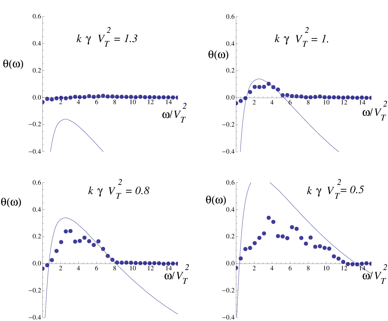
Indeed, to check the predictive power of formula (10), we have run a set of computations where 1000 particles are released slightly above the cell, with $\varepsilon=0.2$ and $\tau=0.02$. The trajectory of each particle $p$ is then calculated by introducing a random phase shift $a_{p}$ in the flow perturbation (simply replace $\omega t$ by $\omega t+a_{p}$ in equation (2)). The calculation is stopped when the particle reaches a fixed bottom, below the cell. We then calculate the centred averaged path length :

$$\theta(\omega)=\frac{L(\omega)-L(\infty)}{L(\infty)}$$

where $L(\omega)$ is the average particle path. The quantity $\theta(\omega)$ is plotted in figure 6 for four values of $V_{T}$. In addition, we have plotted the amplitude of the Melnikov function minus its constant part, that is $F(\omega/V_{T}^{2})-k\gamma V_{T}^{2}$, the positiveness of which implies chaotic particle motion. It appears that when $F(\omega/V_{T}^{2})-k\gamma V_{T}^{2}<0$ the average particle path length is closed to zero (i.e. all the particle paths have roughly the same length), as expected if the two manifolds do not intersect (like in figure 2(c)). In contrast, a soon as $F(\omega/V_{T}^{2})-k\gamma V_{T}^{2}>0$ the average particle path length increases, and this manifests the fact that some particles have penetrated into the cell, as a consequence of the homoclinic bifurcation.

The calculations presented in this note show that a fixed vortex is sufficient to induce chaotic particle motion, under the sole effect of gravity and of the unsteadiness of the vortex. We have chosen to consider a fixed vortex with time-dependent intensity. One could argue that this choice is not realistic, since the intensity (circulation) of vortices is known to remain constant unless viscosity affects it (Kelvin’s theorem). This is why we assumed that some appropriate boundary conditions, or an appropriate volumic force, was present to sustain the whole picture. Our goal being to show that gravity and unsteady differential rotation are sufficient ingredients to induce chaotic particle settling. Note also that the detailed shape of the vortex (here a rotation rate decaying like $1/r^{2}$, where $r$ is the distance to the vortex centre) might not be of major importance, and that other decaying rotation rates could also lead to chaotic particle motion.

In the present analysis, gravity plays a significant role since it is responsible for the appearance of a homoclinic trajectory in the leading-order dynamics. Like for particle settling in the vicinity of upward streamlines[1], particle inertia is opposed to the appearance of chaos, because of centrifugal effects, and tends to maintain the two invariant manifolds $W^{s}$ and $W^{u}$ away from each other. The flow unsteadiness, in contrast, tends to make these manifolds intersect.

To check the predictive power of the Melnikov analysis we have computed the average length of particle paths, as proposed by Ziemniak & Jung [20] in the framework of fluid points trajectories in the wake of a cylindrical obstacle. These authors observed that the probability to find a trajectory whose path length increase is larger than some value $s$, is an exponential function of $s$. It would be therefore of interest to check whether such exponential distributions are visible also in the present case. Clearly, these statistics are linked to the area of the lobes (i.e. subsets of the phase space located between $W^{u}$ and $W^{s}$, as shown in grey on figure 2(b)), which can be calculated from the Melnikov function. In addition, lobe dynamics can be used to calculate other global quantities like particle flux accross the separatrices (see for example Rom-Kedar, Leonard & Wiggins [15], Balasuriya [5]). A detailed analysis of such integral quantities would therefore be of interest to characterize more precisely inertial particle transport in the chaotic regime. Further studies on this topic should be of interest.

In the absence of particle inertia ($\tau_{p}=0$) the particle dynamics is always chaotic (just set $k=0$ in the Melnikov function (9)) : this is a pure hamiltonian chaos, in the sense that the complete system is hamiltonian here, and very close to chaotic advection of perfect tracers. The Poincaré sections in this case are very classical, and are shown in figure 7 in the case $V_{T}=1$. As expected, KAM curves are visible outside the stochastic layer close to the homoclinic trajectory, indicating that some particles could be trapped for a while, and these curves are destroyed as the unsteadiness of the flow increases.

The present mechanism could be applied to mixing devices in chemical engineering processes, where one could leave sedimentation act between every two stiring periods. To our knowledge, detailed mathematical analyses devoted to such devices have not been published so far. In another context, the stretch, sediment and fold mechanism could play a non-negligible role in the mixing of plankton (or the mixing of any other "particle") in the upper ocean. Indeed, under the combined effect of settling and of unsteady wind-induced (or temperature gradient induced) rotating flows, patches of sedimenting particles could perhaps be mixed efficiently. This point needs further discussions.

The main conclusion of the present work is that an unsteady differential rotation is sufficient to induce chaotic heavy particle settling provided the still-fluid terminal velocity of the inclusion is close enough to the flow velocity, and particle inertia is small enough. (In contrast, fluid point trajectories are very regular here, as fluid points go to and fro along portions of circle.) The mechanism, which can be called "stretch, sediment & fold", is sketched in figure 8 (for the sake of clarity, large amplitude oscillations are assumed there) : a particle cloud is stretched by a vortex, then the vortex weakens and the cloud sediments, then the vortex starts again and the cloud is folded, and so on. This elementary mechanism is different from the one investigated by Vilela & Motter [18] with two blinking vortex-sources. Indeed, in the system investigated by these authors gravity is not a key ingredient for the appearance of chaos. The particle spirals out around the vortex-sources, until it reaches a limit cycle and remains suspended permanently. On this attractor the spiraling time of the inclusion is of the order of the period of the blinking. In our single-vortex case, it is the sedimentation time scale which has to match the blinking period. Moreover, these authors show that a cascade of period doublings occurs as the particle inertia decreases, leading to a strange attractor. In the present paper no attractor can be observed, since our system is reduced to a perturbed hamiltonian system. It could therefore be of interest to check whether, once this simplification is removed, a permanent suspension could appear in the vicinity of a single fixed singularity with time-periodic strength, and gravity. Further analyses should clarify this point.

References

- [1] J.R. ANGILELLA. Asymptotic analysis of chaotic particle sedimentation and trapping in the vicinity of a vertical upward streamline. Phys. Fluids, 19(7):073302, 2007.
- [2] H. AREF. Stirring by chaotic advection. J. Fluid Mech., 143:1–21, 1984.
- [3] H. AREF. The development of chaotic advection. Phys. Fluids, 14(4):1315–1325, 2002.
- [4] V. ARNOLD. Sur la topologie des écoulements stationnaires des fluides parfaits. C. R. Acad. Sci. Paris A, 261:17–20, 1965.
- [5] S. BALASURIYA. Optimal perturbation for enhanced chaotic transport. Physica D, 202:155–176, 2005.
- [6] J. DAVILA and J. HUNT. Settling of small particles near vortices and in turbulence. J. Fluid Mech., 440:117–145, 2001.
- [7] J.C.H. FUNG. Gravitational settling of small spherical particles in unsteady cellular flow fields. J. Aerosol Sci., 5:753–787, 1997.
- [8] J. GUCKENHEIMER and P. HOLMES. Non-linear oscillations, dynamical systems and bifurcation of vector fields. 1983. Springer.
- [9] M. HENON. Sur la topologie des lignes courant dans un cas particulier. C. R. Acad. Sci. Paris A, 262:312–314, 1966.
- [10] J.B. MACLAUGHLIN. Particle size effects on lagrangian turbulence. Phys. Fluids, 31(9):2544–2553, 1988.
- [11] M. R. MAXEY. The gravitational settling of aerosol particles in homogeneous turbulence and random flow fields. J. Fluid Mech., 174:441–465, 1987.
- [12] M. R. MAXEY and S. CORRSIN. Gravitational settling of aerosol particles in randomly oriented cellular flow fields. J. Atmos. Sci., 43(11):1112–1134, 1986.
- [13] J. M. OTTINO. The Kinematics of Mixing : Stretching, Chaos and Transport. Cambridge University Press, Cambridge, 1989.
- [14] J. M. OTTINO. Mixing, chaotic advection and turbulence. Annu. Rev. Fluid Mech., 22:207–53, 1990.
- [15] V. ROM-KEDAR, A. LEONARD, and S. WIGGINS. An analytical study of transport, mixing and chaos in an unsteady vortical flow. J. Fluid Mech., 214:347–394, 1990.
- [16] J. RUBIN, C.K.R.T. JONES, and M. MAXEY. Settling and asymptotic motion of aerosol particles in a cellular flow field. J. Nonlinear Sci., 5:337–358, 1995.
- [17] Y. TSEGA, E. MICHAELIDES, and E.V. ESCHENAZI. Particle dynamics and mixing in the frequency driven kelvin cat eyes flow. Chaos, 11(2):351–358, 2001.
- [18] R.D. VILELA and A. E. MOTTER. Can aerosols be trapped in open flows ? Phys. Rev. Let., 99(264101), 2007.
- [19] L.P. WANG, M.R. MAXEY, T.D. BURTON, and STOCK D.E. Chaotic dynamics of particle dispersion in fluids. Phys. Fluids A, 4(8):1789–1804, 1992.
- [20] E.M. ZIEMNIAK and C. JUNG. Pathlength statistics in passive transport in a flow. Physics Letters A, 1995.