Structural relaxation of polydisperse hard spheres: comparison of the mode-coupling theory to a Langevin dynamics simulation
Abstract
We analyze the slow, glassy structural relaxation as measured through collective and tagged-particle density correlation functions obtained from Brownian dynamics simulations for a polydisperse system of quasi-hard spheres in the framework of the mode-coupling theory of the glass transition (MCT). Asymptotic analyses show good agreement for the collective dynamics when polydispersity effects are taken into account in a multi-component calculation, but qualitative disagreement at small when the system is treated as effectively monodisperse. The origin of the different small- behaviour is attributed to the interplay between interdiffusion processes and structural relaxation. Numerical solutions of the MCT equations are obtained taking properly binned partial static structure factors from the simulations as input. Accounting for a shift in the critical density, the collective density correlation functions are well described by the theory at all densities investigated in the simulations, with quantitative agreement best around the maxima of the static structure factor, and worst around its minima. A parameter-free comparison of the tagged-particle dynamics however reveals large quantiative errors for small wave numbers that are connected to the well-known decoupling of self-diffusion from structural relaxation and to dynamical heterogeneities. While deviations from MCT behaviour are clearly seen in the tagged-particle quantities for densities close to and on the liquid side of the MCT glass transition, no such deviations are seen in the collective dynamics.
pacs
64.70.Pf,82.70.Dd,61.20.LcI Introduction
Understanding the slow dynamical processes occurring in supercooled glass-forming liquids is still one of the challenges in condensed matter physics. The mode-coupling theory of the glass transition (MCT), introduced in 1984 by Bengtzelius, Götze, and Sjölander and Leutheusser [1, 2], provides a quantitative description of the initial slowing down of structural relaxation, when approaching the glassy state from the liquid region. The theory predicts an ideal glass transition whose signature is a two-step relaxation of dynamical density correlation functions. It arises from a divergence of two time scales connected with the intermediate relaxation ascribed to relaxation of particles inside their neighbor-cages (the relaxation), and with the final escape of particles from their initial positions that restores liquid-like motion (the relaxation process). Two hallmarks of glassy dynamics, viz. nonexponential, “stretched-exponential” relaxation and its scaling (also known as “time-temperature superposition principle”), are predicted as asymptotic results of MCT. The theory stimulated many experiments specifically to address the dynamical window for which the theory was designed; among them dynamic light scattering performed on colloidal systems, Brillouin and neutron scattering, dielectric spectroscopy, and computer simulation studies (see Ref. [3, 4, 5, 6] for reviews).
However, MCT is based on the ad-hoc assumption that the fluctuating forces (the longitudinal projections of the microscopic stresses for a particular wave vector ) are governed entirely by the dynamics of density pair fluctuations. To close the equations, one then further approximates a dynamical four-point average through a product of density correlation functions. Even though the theory has had many successes in describing some key features of the slow dynamics, often validated through comparison of its asymptotic formulæ with experimental and simulation data, the accuracy of the MCT approximation is still largely unknown. In molecular glass formers, the fact that relaxation times do not diverge at the MCT transition, but continue to grow smoothly in a regime where motion is thought to be no longer liquid-like but governed by activated, so-called “hopping”, processes, is the most widely criticized manifestation of the approximate nature of MCT. Another commonly quoted feature that is not contained in the theory are the non-Gaussian distributions of particle displacement discussed in terms of dynamical heterogeneity [7, 8]. This effect is often linked to the appearance of a decoupling of viscous and diffusive time scales – the breakdown of the Stokes-Einstein relation, although it could be argued that not its breakdown at low temperatures, but rather its validity at higher temperatures in complex glass formers is the surprising feature.
If hopping processes are indeed what is missing in MCT, checking the feasibility of creating an atomistic model system where such effects are absent, is an obvious thing to do. Following the pioneering dynamic light-scattering experiments on colloidal hard-sphere-like suspensions by Pusey, van Megen and coworkers [9, 10, 11, 12, 13], hard spheres with Brownian short-time motion have sometimes been quoted in this regard. Yet, this exceptional nature of the hard-sphere glass transition has been challenged based on computer simulation of tagged-particle density correlation functions [14]. In this contribution, we wish to analyze the situation further by shifting focus from the incoherent quantities to the collective density correlation functions that are closer to the framework of MCT. We find that, a number of commonly discussed shortcomings of the theory appears only in the tagged-particle but not in the collective dynamics.
One strength of MCT is that it allows, in principle, to predict detailed information on the slow dynamics when given only the particles’ interaction potentials, in the form of the static structure factor, as input. For real-world glass formers, generally mixtures or moderately complicated organic molecules, resolving all the partial static structure information required is a formidable task. Even more so if one is interested not only in the static structure, but also the corresponding dynamical relaxation functions. Thus, in many experimental studies, MCT results were taken either from asymptotic expansions (that cannot address the molecular details and preasymptotic corrections, which may be strong), or from schematic simplifications of the theory’s equations (resulting in a set of fit parameters whose physical meaning is rather unclear). Only recently has it become possible to perform MCT calculations based on actual experimentally measured partial structure factors, due to advances in neutron scattering techniques on liquid metallic melts [15].
Thus, testing the “full MCT”, that is, putting to test the dynamics as calculated within the theory from the static structure factor (without invoking asymptotic or schematic limits of the theory’s equations) against the measured one, is a task for molecular dynamics simulations, and has been performed on the standard glass-forming binary Lennard-Jones mixture [16, 17, 14, 18], on hard-sphere mixtures [19, 20], soft spheres with short-ranged attraction [21, 22], and in more complicated systems such as network-forming strong liquids [23, 24], metallic glasses [25], polymer melts [26], or computer models of organic glass formers such as ortho-terphenyl [27, 28]. As it turns out, these systems are already quite demanding for MCT, although the theory fares well in a qualitative description of the dynamical phenomena, sometimes even quantiatively (most notably, Ref. [23], where also static triplet correlation functions have been extracted from simulation and fed into MCT, addressing a term in the MCT equations whose existence is often silently ignored).
The most simple model for a classical dense liquid is arguably the hard sphere system. In a previous study, we addressed a test of MCT for this system partially, by comparing MCT and molecular dynamics simulations for a polydisperse quasi-hard sphere system [29]. There, however, computational limitations in acquiring the desired statistics restricted the discussion to the single-particle dynamics (in form of the incoherent density correlation functions and quantities derived from it, such as the mean-squared displacements or diffusion coefficients). It should be stressed that MCT is, in its very essence, a theory for the collective slowing down caused by a feedback mechanism for the collective, or coherent density correlation functions. Calculating tagged-particle dynamics from this viewpoint involves an additional level of (MCT-approximate) equations, and can thus be viewed as a more indirect way of testing the theory. In this paper, we complete the task of Ref. [29] by detailing a comprehensive, quantitative comparison of MCT with molecular dynamics computer simulations for the same quasi hard-sphere system on the level of the collective density correlation functions. Additionally, while in Ref. [29] an approximate liquid-state theory for the static structure factor input to MCT was used (the Percus-Yevick approximation), we avoid this additional non-MCT level of approximations by using directly the simulated static structure factors.
Comparing the dynamics to MCT, it should be recognized that the theory focuses on the slow structural relaxation, mistreating the short-time dynamics as governed by uncorrelated binary collisions (whose inclusing into the theory is not straightforward [16, 17]). It is thus desirable to minimize the influence of this short-time dynamics, in particular since its details do not change those of the long-time relaxation [30, 31]; it turns out that this is achieved by including stochastic noise in the simulated equations of motion, leading to a Langevin-dynamics simulation. Standard molecular-dynamics integration is then most easily implemented using a regular soft-sphere potential, . For such steep power-law potentials, it is known that the influence of slight ‘softness’ on the dynamics can be mapped to an effective density in a mapping that takes into account the according shift of the freezing point [32]. In addition, the stochastic dynamics provides a link to experimental data on colloidal hard-sphere-like systems, whose Brownian short-time dynamics we mimick in our simulations.
Monodisperse hard- or soft-sphere systems beyond the freezing point readily crystallize in simulation. To avoid this, we take the spheres’ radii to be polydisperse, evenly sampled from a narrow distribution just wide enough to suppress crystallization on the time scales considered in our simulations. It is well known that already small polydispersities are very efficient in slowing down nucleation events dramatically [33, 34]; polydispersity is also inherent to most colloidal suspensions, making it a natural feature to consider. Binary mixtures are another common way of circumventing unwanted crystallization, but polydisperse systems have the advantage that one can meaningfully construct species-averaged total correlation functions that are not too different from the individual partial correlations. In principle, this allows to greatly simplify the discussion, by applying the original one-component formulation of MCT. However, polydispersity may play an interesting role when comparing theory and simulations in particular at small wave numbers . We will discuss these points in detail below, including three- and five-component moment approximations to the polydisperse radius distribution in multi-component MCT [35, 36]. Comparing with the one-component MCT, this addresses the question of static versus dynamic averaging: while the true dynamics of the system can be mapped onto an effective one-component system only by averaging at the level of the dynamical correlation functions (a procedure to which we will refer as post-averaging), it is tempting to perform such averaging over a narrow polydispersity distribution already on the level of the static structure factor (pre-averaging). However, as we will discuss, the nonlinear feedback effects of the dynamics pose a limit to the validity of such an approach.
The paper is organized as follows: In Section II the features needed in the further analysis of both MCT and simulation are reported for reference. Section III demonstrates purely asymptotic analyses of the simulation data, while Sec. IV turns to the full MCT description of the simulated dynamical correlation functions. Finally, in Sec. V we summarize.
II Simulation and MCT
II.1 Molecular-dynamics simulation
We perform strongly damped molecular-dynamics (Langevin-dynamics) simulations mimicking colloidal Brownian dynamics (BD). The core-core respulsion between particles and is given by
| (1) |
where is the center-to-center distance, , with the diameters of the particles, sampled from a uniform distribution centered on the mean diameter with half-width . Such a soft-sphere system has only one control parameter given by a specific combination of number density and temperature , [37]. We vary by keeping the temperature fixed and changing the system’s density. It has been shown [32] that the exponent of the inverse power-law potential is large enough to effectively approximate hard-sphere behavior.
The equation of motion for particle is given by the Langevin equation,
| (2) |
which contains the direct forces between particles , and stochastic and friction forces, with friction coefficient , modeling interaction with a solvent. Assuming Stokes friction, its value would be connected to the solvent viscosity , , where is the hydrodynamic diameter of the particle (approximated as equal for all particles, since the spread in the is small). The random forces fulfill the fluctuation-dissipation theorem, . Let us note that with the value of chosen in our simulations, the short-time dynamics visible in the correlators and in the mean-squared displacement is not yet completely overdamped, i.e., it is not strictly diffusive, but rather strongly damped ballistic. Since it is not our aim to investigate the very short-time dynamical features of the simulations, this will not be discussed in the following.
Equilibration runs were performed with undamped Newtonian dynamics in all cases, since the damping introduces a slowing down in the overall time scale. particles are simulated in a cubic box with standard periodic boundary conditions. Lengths are measured in units of the mean diameter , the particle mass , and the unit of time is fixed setting the thermal velocity to . The damping was chosen as in these dimensionless units, and the equations of motion were integrated following Heun’s algorithm [38] with a time step of . Due to the polydispersity, crystallization did not occur in the runs that have been analyzed for the following discussions. Crystallization was monitored through the orientational order parameter [39, 40]. It was found that out of runs for , and out of runs for in fact did crystallize and had to be excluded. Density is reported as volume fraction, , where the polydispersity has been taken into account. Volume fractions investigated in the following are , , , , , and . In all states or different systems were prepared from scratch, and or independent correlation functions were measured adding to a total statistics of evaluations of the dynamical quantities per state.
In order to study the specific effects of polydispersity, a varying number of bins has been used to group particles according to their size: besides the usual effective one-component analysis, , we also discuss a three-component, , and a five-component, , interpretation of the data. In these cases, bins of uniform width have been chosen. We mainly discuss the collective density correlation functions (intermediate scattering functions),
| (3) |
whose equal-time values are the partial static structure factors . Here, indices label the component bins containing particles, and are the collective partial-number-density fluctuations at wave vector , where is the position of the k-th particle of species . Note that these correlation functions are real-valued and depend on only through its scalar invariant , as the system is isotropic and translational invariant. The brackets indicate time-origin or canonical averaging in the simulation or theoretical approach, respectively. To improve the statistics of this function, a small dispersion in -modulus was allowed for, for and for . The change in can be noted as a kink in some wave-vector dependent quantities derived from it at .
Additionally, we measure the tagged-particle (incoherent) density correlation functions, i.e., the self-intermediate scattering function
| (4) |
where denotes the Fourier transformed one-particle density. In this case, averaging over all particles of the same species allows to further improve statistics in the simulation. is connected in the low- limit to the mean squared displacement of species ,
| (5) |
The “polydispersity-averaged” total correlation functions are recovered by summing over the bins,
| (6) |
which in the tagged-particle correlation function reduces to
| (7) |
and the analog expression for the mean-squared displacement,
| (8) |
II.2 Mode-coupling theory
The mode-coupling theory for -component mixtures builds upon an exact equation of motion derived for the matrix of the partial dynamical density correlation functions defined in Eq. (3). Applying Zwanzig-Mori projection operators to the Liouville equation governing the microscopic dynamics, one arrives at [35]
| (9) |
with and the memory kernel matrix which embodies the fluctuating quantities and plays the role of a generalized friction coefficient. Note that in our case, is the same for all pseudo-species. Initial conditions for the equations of motion are and . We split the memory kernel into a contribution describing the regular part of the friction, modeled as a Markov process with a damping coefficient that is chosen in agreement with the one taken in the simulations, and a collective part describing the slow dynamics,
| (10) |
where with . MCT now approximates as a nonlinear functional of the density correlation functions,
| (11) |
with components
| (12) |
The vertices couple the density fluctuations of different modes, with ,
| (13) |
Here we have additionally approximated static three-point correlation functions in terms of two-point ones. Their inclusion is computationally too demanding and does not change the results strongly in dense, non-network forming systems such as ours [23]. is the matrix of direct correlation functions defined through the Ornstein-Zernike equation
| (14) |
Thus, taking from simulation, the collective dynamical density correlators are fully determined in the theory.
The tagged-particle correlator for a singled-out particle of species obeys an equation similar to Eq. (9),
| (15) |
with and the initial conditions , . We set to obtain damped-Newtonian short-time dynamics. The corresponding memory kernel is evaluated from Eqs. (12) and (13) by considering a (M+1)-component mixture in the limit of one concentration going to zero:
| (16) |
with the tagged-particle vertex
| (17) |
As the memory kernel in Eq. (16) contains the coherent correlator, solving Eq. (15) requires the full coherent dynamics to be known.
By virtue of the expansion , the mean-squared displacement of species is connected to the tagged-particle correlator via
| (18) |
Its equation of motion follows from Eq. (15):
| (19) |
with and
| (20) |
Equation (20) states that the mean-squared displacement is completely determined from the collective and tagged-particle density correlation functions; there is no back-coupling of the MSD to itself since the phase space at has vanishing contribution inside the integral.
Many features of the solutions of the above MCT equations are known, especially concerning points asymptotically close to MCT glass transitions. We only summarize the basic results for completeness, referring to the literature [41, 4, 42, 43] for details. The starting point of the asymptotic analysis is to realize that the MCT equations allow for bifurcation points for the long-time limit of their solutions. Denoting them by
| (21) |
one finds that these long-time limits (synonymously called glass form factors or nonergodicity factors) are determined by a set of coupled, implicit nonlinear equations,
| (22) | |||
| (23) |
In the usual case, it is Eq. (22) that displays bifurcations: Out of the possibly many solutions to this equation, the long-time limit corresponds to the non-negative real solution that is largest according to a straightforward ordering defined for each separately and through the positive-definiteness relation [44, 45]. The glass transitions of MCT are then the bifurcation points affecting this largest solution that arise from smooth changes in the control parameters, and the most common case is that of a bifurcation where the long-time limit jumps discontinuously from the trivial zero solution indicating a liquid to a finite value indicating a solid. The solution determined as the largest solution of Eq. (23) will then, in the generic case, inherit the bifurcations of , and we will not discuss the possibility of extra singularities arising in Eq. (23) itself. The generic case is in particular obeyed by the problem at hand, quasi-hard-sphere tracer particles inside a quasi-hard-sphere system composed of particles of roughly equal size. Generally, the transition points are then defined as the points where the stability matrix of the nonlinear Eq. (22), given by
| (24) |
has a unique critical eigenvector with eigenvalue unity. is also called the critical amplitude (up to trivial normalization factors that are sometimes split off from it). We will denote quantities corresponding to such a transition point with superscript, e.g., and .
On the liquid side of the transition, correlation functions follow a two step relaxation scenario: for times large compared to the characteristic time of the short-time motion, , they decay with a time fractal to the plateau, which extends until the -relaxation time scale . For , the decay from the plateau sets in with the von Schweidler law, , initiating the final relaxation that is characterized by a second time scale . The asymptotic analysis proceeds by analysing the equation of structural relaxation, where time-derivatives that affect only the short-time motion have been dropped,
| (25) | |||||
Identifying the distance of the correlator to its plateau value as a small parameter , one extracts the two time scales that diverge upon letting ,
| (26) |
where , and and are nontrivial and nonuniversal exponents determined by the details of the interaction potential (see below). The separation parameter is, in leading order, linearly connected to the change in control parameters, viz. in our case with . By convention, indicates a liquid state, the glass. Note that also diverges as , so that asymptotically close to the MCT transition, an ever larger window for structural relaxation around the plateau open. In practice, this window is cut short for large by preasymptotic corrections, and for small when the theory fails to describe residual ergodicity-restoring processes in the glass.
For times where the correlator is close to one makes the following Ansatz
| (27) |
and the uniqueness of the critical eigenvector at the bifurcation point implies the factorization theorem, . The function is determined by the so-called -scaling equation
| (28) |
The nonuniversal details of the vertices enter in this equation only thorugh the exponent parameter,
| (29) | |||||
where , and the double-dot operator includes contraction over . Here, is the left-eigenvector corresponding to .
For times the decay to the plateau at the critical point is then governed by the -relaxation; in leading order,
| (30) |
where is determined as solution of
| (31) |
For times and for the decay of the correlator is described by the von Schweidler law
| (32) |
Here , the von Schweidler exponent is determined from the negative solution of Eq. (31).
In the glass () the nonergodicity parameters behave like
| (33) |
Again we define the “polydispersity-averaged” total nonergodicity parameters and the total critical amplitudes by summing over the bins,
| (34) |
For timescales and the -master equation can be derived
| (35) | |||||
This equation states that all correlators should collapse on the same function when rescaled by an appropriate scaling time . This is due to the invariance of Eq. (35) when rescaled in time and is the mathematical manifestation of the time-temperature superposition principle.
II.3 Numerical details of the MCT solution
MCT calculations were performed with static structure factor matrices taken from the simulations; to access packing fractions for which no simulations have been run, linear interpolation in was used for . As in the simulation, calculations with a one-component (), and two different multi-component binnings, and , have been performed (see Sec. II.1). To choose effective diameters for the different bins, we have followed the moment approximation [35, 36]: for , the three values and equal concentrations allow to match the actual polydispersity distribution up to the second moment (with the requirement that the skewness of the distribution vanishes), and for , additionally the fourth central moment can be matched using equal concentrations. This leads to the choice in the system, and for the system.
The problem of solving Eq. (9) in full has to be tackled numerically, choosing a suitable discretization. The wave number grid selected here is in steps of . The discretization is a compromise between calculation time and being as close as possible to the simulation structure factors. The initial time step was chosen as . After every steps the stepsize was doubled in order to cover logarithmically large intervals in .
III Data Analysis
III.1 Structure factors

We first address the static structure factor that serves as an input to MCT, and obtained from the simulations. In Fig. 1, the averaged structure factor is shown for different packing fractions. It exhibits the standard features known for dense liquids where excluded volume is the main interaction effect: a pronounced first peak is visible that shifts to higher -values and increases in intensity with increasing packing fraction, reflecting a decreasing average next-neighbor distance and increased local ordering in the denser system. The figure also includes as calculated from the Percus-Yevick (PY) approximation for monodisperse hard spheres [46]. It is known that this approximation performs quite well, but somewhat over-estimates the amount of ordering present in the system; this is expressed by a shift in density values. Still, comparing densities where the first main peak is reasonably well described within PY, the amplitude of the second peak in is notably overestimated by the approximation in comparison to our simulation results. Note that in MCT, the main contribution to the memory kernel causing slowing down and arrest comes from these amplitudes in . As larger wave numbers contribute more strongly to the three-dimensional integral, not just the main peak of , but also the shape of its large- envelope determine the MCT dynamics; one can thus anticipate from Fig. 1 that MCT calculations based on the PY structure factor will clearly underestimate the critical packing fraction.

In Fig. 2, we show the partial structure factors resulting from a binning of the simulation data into a three-component system. All diagonal terms as well as the off-diagonal terms (except for a trivial shift by the constant ) are very similar as expected for a mixture of almost equal constituents. The slightly different average next-neighbor distances for the different particle sizes cause corresponding shifts in the oscillation frequencies and hence the positions of the peaks in . This effect is most pronounced in the diagonal terms, as these only contain information from one distinct particle-size bin. Adding these partial structure factors recovers the shown in Fig. 1, and elucidates that the comparatively weak high- peaks visible there are the result of a destructive interference of the slightly shifted oscillations in the multi-component . However, the main peak is strong enough to be less affected. Thus, for systems whose interactions are close to hard-core repulsion, such as our system, averaging mainly results in an underestimation of the coupling strength, i.e., too fast dynamics in the one-component calculation as compared to a multi-component calculation. Indeed, our MCT calculations discussed below essentially confirm this expectation, that in the range of around the first peak in and above, the changes between pre- and post-averaging are minor once the shift of the critical packing fraction is acocunted for. Yet, for small , the situation is more intricate. Let us also note that for systems whose glass transition features are dominated by the large- behavior of the static structure factor, the destructive interference induced by pre-averaging the MCT input can lead to severe changes in the qualitative dynamics [21]. This particularly concerns polydisperse colloid-polymer systems with short-ranged (depletion-induced) interaction among the colloids.
III.2 Critical point density
| model | ||||
|---|---|---|---|---|
| 0.566 | 0.717 | 0.613 | 0.320 | |
| 0.537 | 0.735 | 0.583 | 0.315 | |
| 0.535 | 0.739 | 0.576 | 0.310 |
The critical packing fraction of the MCT glass transition was calculated with a bisection algorithm which returns the point where the eigenvalue of the stability matrix , Eq. (24), is unity. Table 1 summarizes the values of along with the corresponding exponent parameters and the MCT exponents corresponding to these values, for the , , and calculations we performed.
As expected from the discussion of the static structure factor above, the glass transition point in the calculations shifts to lower densities with increasing . Remarkably, the most pronounced change already occurs between and , whereas the further increase to does not alter or substantially. We thus consider to be already close to the limit of many components that should in fact be taken to describe a truly polydisperse system. At this point we would like to stress that the downshift of the glass transition point for is only related to the different MCT-models used here, as the polydispersity in the simulation is not changed. It should be noted that still, even the value is significantly above the value calculated within the PY approximation, [42]. However, the MCT glass transition from an asymptotic analysis of the simulation data yields a value [29], much higher than the values calculated within the theory even with the correct static structure information, but in reasonable agreement with the commonly quoted value for polydisperse hard-sphere like colloidal suspensions, [47]. This is a well known shortcoming of MCT, and we consider the better agreement we obtain for the one-component calculation, as fortuitous. Note also that one usually expects polydispersity to shift the glass transition to higher densities, as the overall packing efficiency incresases [48]. However, the role played by the different shapes of the polydispersity distributions is not well studied. Within MCT, this commonly observed trend of increasing in mixtures is, at least for binary hard-sphere mixtures, only predicted for size ratios , while for closer to unity, the inverse trend is found [36]. Relating to the extreme in our calculations, even our system only corresponds to .
III.3 -process analysis
Next, we test the validity of scaling for our simulation data. According to Eq. (35), plotting correlators as functions of should collapse the data for long times, with a master curve extending as from below.

To determine a relaxation time from the data alone, we have shifted the correlation functions at a single fixed value of to coincide with the corresponding curve at the highest packing fraction in the liquid, , at long times. After this procedure, the validity of the scaling can be checked by requiring that be independent on . Note that corresponds to the position of the main peak in the averaged static structure factor. We have chosen this value since here the strength of the process is maximal, and the best separation from the regime is achieved. Fig. 3 shows the result of this scaling for four different wave numbers. An -master curve clearly is approached, with the scaling regime for the highest two densities extending over about two orders of magnitude in time. The strong coupling of the -relaxation on local length scales predicted by MCT is observed, as the same scaling factor rescales the correlators for different wavevectors.
In the lower panel of Fig. 3, the scaling is exhibited for small ; here, deviations are visible at , where the simulation data does not exhibit a common shape for the -relaxation part of the correlators. The highest shown indicate a decay that is either more stretched or exhibits a further inflection point in the -versus- plot below the plateau. We will return to such features below in the discussion of hydrodynamic interdiffusion modes that exist in multi-component systems and interplay with the structural relaxation at low .
A common description of the shape of the relaxation is in terms of stretched-exponential (Kohlrausch) laws,
| (36) |
Here, is the stretching index, required to be for structural relaxation in equilibrium systems. While the -master function from MCT is different from the Kohlrausch form, the theory predicts that for large wave numbers, the two functional forms become identical, and [49]. is commonly referred to as the -relaxation time, and it is connected by a -dependent but density-independent prefactor to the scaling time appearing in MCT. The Kohlrausch amplitude can be taken as an estimate of the MCT plateau value , and since the process by definition starts below this plateau, is expected. In practice, however, the separation of the process from the relaxation is often not clear enough to warrant this restriction.

In general, Kohlrausch fits are hindered by some subtle problems that are often overlooked. Lacking a clear separation of the process, the fit parameters exhibit a dependence on the fit range. It is not clear a priori how to choose the optimal fit range, as for very long times, one expects the relaxation to become (non-stretched) exponential again (and to be covered within the noise of any experiment), and for short times, deviations are seen that can be understood within MCT to be due to the difference between and for finite .
We have tried to fix the fit range of our stretched-exponential fits such that the fit parameters exhibit only a weak dependence on the fit boundaries. Examining the correlators for , this leads to . In Fig. 4, examples of such fits are shown. Although the agreement is generally convincing, let us stress that these fits are a pure data analysis, not taking into account the full numeric MCT calculations we will discuss below. The curves in Fig. 4 show what one can extract parameters like the plateau value or the von Schweidler exponent without having performed full MCT calculations. In Fig. 4, we additionally show the results of von Schweidler fits to the simulation data: adapting Eq. (32) and extending it by the next-to-leading order [42], we fitted
| (37) |
determining , , and by fitting and fixing to be consistent with the analysis of -relaxation stretching presented below (Fig. 8). Note that a free fit of von Schweidler’s law without fixing is usually ambiguous as the determination of the MCT exponents directly from data bears uncertainties [50]. Eq. (37) has been used in the range . The von Schweidler results then represent about two decades in time of the correlation functions.

Figure 5 shows the results for the amplitude , together with the nonergodicity parameters calculated from MCT, and the estimates of obtained from von Schweidler fits. The values obtained from all three methods in general show good agreement, although some details warrant discussion. Let us first turn to the large- regime, . Here, the von Schweidler fits, Eq. (37), yield that are in good agreement with the Kohlrausch amplitudes , and the relation is reasonably well fulfilled. The MCT calculations somewhat underestimate , although the agreement is soupcon improved for the multi-component systems with and , in particular for values of where the averaged static structure factor (and hence also the -versus- curve) shows minima. The underestimation of by MCT can be attributed to the underestimation of : MCT describes arrest at lower densities, but increases with density as the denser glass is stiffer with respect to density fluctuations. For comparison, we also show in Fig. 5 the obtained by employing the PY approximation within MCT; this result agrees well with the and calculations, indicating in particular that for the arrest of small-wavelength fluctuations, polydispersity and particle softness do not play a major role. One in fact recognizes that the truly monodisperse calculation (with PY input) is in better agreement with the polydisperse data than the one-component calculation using the polydispersity-averaged . This can be intuitively interpreted: pre-averaging in artifically reduces large- static correlations, but is in essence a dynamical quantity, and the effect of the dynamics on these large- correlations needs to be included to describe the degree of dynamical arrest. Still, in Fig. 5 this is a merely quantitative effect.
For the large-wavelength regime, , the situation is more differentiated: here, both one-component calculations differ more notably from the results obtained by pure data fitting, and the results calculated with the or theory. In particular, the PY-based one-component result shows a rather weak -dependence of the plateau value for small , and yields in this regime. In contrast, the multi-component results show an upturn of as is decreased, with plateau values rising to almost at the lowest accessible in the simulation. The one-component MCT calculation based on the simulated (pre-averaged) structure factor also shows this upturn, but less pronounced.
This behavior can be rationalized by the effect of polydispersity: first, going over from the strictly one-component PY approximation to the simulated already contains static, pre-averaged information about the size distribution, and this is sufficient to explain qualitatively that polydispersity tends to increase the stiffness of the frozen structure towards long-range density fluctuations. The post-averaged calculation is needed to capture this trend quantitatively. It shows that additionally the freezing out of the interdiffusion process increases the average at small [51].

The tagged-particle analog of the quantities shown in Fig. 5, , is exhibited in Fig. 6. Here, the differences in the different methods of determining the plateau height are much smaller, as intuitively expected; the incoherent -versus- shapes do not show the oscillations typical for the collective quantities. Only at the largest wave numbers investigated here, , some differences between the MCT calculation and the fit results become apparent. Here, the theory again underestimates the amount of arrested density fluctuations, and this can agian be rationalized by its lower critical density. For small , all have to approach unity, so that any differences are trivially wiped out.

Let us now turn to a discussion of the -dependence of the relaxation time and the stretching resulting from Kohlrausch fits. To obtain equivalent values also for the MCT curves, we have fitted the theory’s -master curves with stretched exponential functions. Numerically, the master curves have been approximated by correlators close to the transition point: choosing in Eq. (9) proves sufficient to effectively solve Eq. (25) for the timescales of interest. For the simulation, we again restrict the discussion to the highest density available, , which however corresponds to a different . Thus, to enable a meaningful comparison, relaxation times are scaled to coincide at .
Figure 7 shows the resulting -relaxation times for both the coherent (upper panel) and incoherent (lower panel) dynamics. A similar distinction into two regimes as above arises: for , the -dependence of the relaxation time is excellently predicted by the theory. For , this holds for the collective correlation functions only when comparing with the multi-component calculation. Even the pre-averaged one-component calculation is in qualitative difference, since there, approaches a constant, resulting in a weak -dependence for all . Instead, in the multi-component theory, as for every single matrix element of the partial-density correlation-function matrix. This has a clear physical interpretation: reflects the fact that the overall momentum of the system is conserved. However, this is not the case if one considers a single species inside a mixture of components only, since momentum can be exchanged between the species. Only the sum of the partial momenta is thus conserved, which is reflected in the existence of an appropriate zero eigenvector in the MCT memory kernel; however, this does not transcede to the averaged correlator defined by Eq. (6) itself. Strikingly, the resulting rise in as that is apparent in the MCT calculations is in very good agreement with the simulation results, with only the lowest values of the simulation deviating slightly (which may be due to minute finite size effects).
For the same reason (momentum conservation or rather the lack thereof for a single species), is expected in any system. Indeed, this is seen in all curves in the lower panel of Fig. 7. However, the divergence predicted by MCT is stronger than the one seen in the simulation, an effect visible even at finite . Only in the large- regime defined above is the MCT description of the quantitatively accuracte. At the largest extracted from the simulation, the theory in turn somewhat underestimates the relaxation times.

Turning to the stretching exponents , Fig. 8, the agreement between MCT and simulation is less favorable. The values obtained from fitting the theory curves are systematically too high, an effect that will become evident also below when discussing the full correlators. Only the qualitative behavior of with is qualitatively in agreement, although the difficulty of determining in the simulation for large , where the amplitudes are already rather low, does not allow a detailed discussion.
Since the master curve strictly is a Kohlrausch function only in the limit [49], emphasis should mainly be placed on the behavior of at large , and at small , as we will discuss below. For large , the fits to the MCT curves nicely exhibit the asymptotic behavior, , with a value of , consistent with the values given in Table 1. Also the simulation-fitted stretching exponents are compatible with the approach to a finite constant at large , albeit with a somewhat lower value, ; we can take this difference as an indication for the error inherent in the value of as calculated within MCT, in particular since the value of is in good agreement with the that results from an independent -relaxation analysis of the simulation data (see below). For the simulated incoherent correlation functions, however, no such large- limit can be identified for ; the reason for this behavior is unclear.
At low , the appearance of a diffusion mode in the incoherent correlator demands for (since hydrodynamic relaxation functions are just exponentials). The fits to both the different theory calculations and to the simulation data confirm this. For the coherent , no such statement holds in the true monodisperse system; there is no collective single-component diffusion mode. Hence, is found for the MCT calculation based on the pre-averaged structure factor. For the same reason discussed in connection with the behavior above, however, the from fits to the simulation data do exhibit an increase as decreases towards zero. In principle, a similar trend should be found in the multi-component MCT calculations. However, a peculiarity arises here, that prevents us from determining meaningful values of in this case for . Here, the appearance of a number of distinct interdiffusion processes typical for a multicomponent system leads to -relaxation curves that are superpositions of a small number of exponentials, leading to master curves that exhibit multiple “shoulders”; for the corresponding relaxation spectra, this corresponds to multiple peaks [52, 51]. Such interdiffusion processes in principle also exist in the simulation; however in this truly polydisperse system, a large number of them is combined to a relaxation curve that is again reminiscent of a single process (akin to a heterogeneous superposition of single relaxators).
III.4 -process analysis

We complete the asymptotic analysis of our simulation data by investigating the -scaling regime. On approaching , MCT states that the correlation functions be described in leading order by Eq. (27). However, testing this relation involves a number of fit parameters whose determination is difficult. An approach to testing the first main prediction of MCT for the -relaxation window, viz. the factorization theorem, is to consider the function [30]
| (38) |
with times and fixed to be inside the scaling regime. Equation (27) then predicts to be independent on wave number; hence, superimposing the functions for different , one should be able to fix the two times and uniquely such that a time window appears where all collapse. The procedure has the advantage that the critical amplitude drops out and thus does not need to be determined by fitting. It was shown to work very reliably in a binary Lennard-Jones mixture by Gleim and Kob [30].
As shown in Fig. 9, such a collapse is indeed possible for the simulation data at , where we have chosen and . Both the collective and the tagged-particle density correlators collapse for all the wavenumbers investigated for a region spanning and slightly extending to both smaller and larger times. Estimating that (, ) for the (, ) analysis, one cannot expect the first-order asymptotic result for the -relaxation function to hold over more than one decade in time [42]; indeed this is roughly what we observe.
A stronger test of the MCT asymptotics implicit in Fig. 9 is the so-called ordering rule: since in the next-to-leading order corrections to the factorization theorem the same -dependent correction amplitudes appear both for the early-time deviations and for the long-time corrections [42], correlators that lie, say, above the correlator for short times must also deviate in that direction for long times. Thus, numbering the correlators in the order in which they deviate from the asymptote for short times, the same numbering should be found on the long-time side. Figure 9 confirms this. As was also found in Ref. [42] for the MCT calculations based on the PY structure factor for hard spheres, this ordering rule is even preserved among the correlators at long times, when the correlator already violates it. This effect can be seen in Fig. 9 by noting that the leading-order asymptote (drawn as a dashed line) emerges between the and correlators, but already crosses the curves for smaller at around , while the correlators obey the ordering rule up to the time window plotted, .
In order to extract the critical amplitude from the simulation, one can define a function in analogy to Eq. (38) by
| (39) |
with , chosen in the -scaling regime. The last equality follows again from Eq. (27) and thus allows us to extract the critical amplitudes up to a factor . Since Eq. (39) becomes independent on the times chosen as long as they are in the -relaxation window, we can further improve the statistics of by averaging over two time windows [53]
| (40) |
and use all the data points within the -scaling regime, which leads in our case for to .

As a cross-check, we have also determined the critical amplitudes by directly fitting the von Schweidler expression including its leading-order correction to the late regime, as described in conjunction with Eq. (37). Figure 10 shows the results for the critical amplitude of the coherent density correlators, . Reassuringly, both determinations of give results that are fully consistent with each other. Also shown in the figure are the MCT-calculated amplitudes. For all three values of the number of components chosen, , the data are in very good agreement, with strongest deviations setting in for . In particular, the strong dip in around is well reproduced. In general, the shape of the -versus- curve is in this regime quantitatively captured already by the Percus-Yevick approximation discussed in Ref. [42]. At small wave numbers, , deviations set in that are the analog of those discussed above in connection with and : polydispersity affects the long-wavelength fluctuations in the system, and using the pre-averaged static structure factor within MCT cannot describe these mixture-specific features. It is intuitively clear that, since the actual is larger than its one-component estimate at small , the opposite has to hold for , as the normalization of the correlation function implies .

In Fig. 11, the tagged-particle critical amplitudes are displayed. Again, the two procedures to determine this quantity from the simulation data alone agree. The result shows a peak around , while for , follows from hydrodynamic laws. In contrast to the coherent amplitude , for the MCT results show more pronounced deviations from the simulation values. The theoretical quantities exhibit only a weak dependence on the number of component bins in this case, and peak around , i.e., at slightly larger wave numbers than what is observed in the simulation. Generally, a shift of the -versus- curve arises, indicating that MCT gives a wrong estimate of the relevant length scale for the tagged-particle motion in the regime. It is unclear whether this mismatch can be attributed to the mismatch in critical packing fractions between theory and simulation, as was done for . It is also notable that the disagreement is pronounced only in the tagged-particle critical amplitude; absorbing it into an effective wave number, as done in Ref. [29], would in fact worsen the agreement for the collective amplitude as can be seen in Fig. 10.
IV Full MCT-Analysis
Having established the generic MCT scenario for the simulation, we now present the numerical solutions of the full (non-asymptotic) MCT equations. In principle, the dynamical correlation functions thus obtained can be directly compared to the corresponding quantities extracted from the simulation. However, the mismatch in the values neccessitates a comparison not at equal densities, but at, in principle, equal separation from the respective transition points. In the spirit of the MCT asymptotics, a comparison should involve matching the separation parameter ; however, this is not easily determined for the simulation, since the true functional dependence between and the control parameters is not known. Only asymptotically close to the transition do we have , with a pre-factor that also can only be calculated within MCT (and thus might be in error). It is therefore practical to perform a fitting of the packing fractions used in MCT, to the nominal ones used in the simulation, , for each of the MCT systems with a different number of components . We have performed this fitting based only on the coherent correlators at ; the comparison for all other wave numbers, and for all tagged-particle quantities then is parameter-free.
It should be noted that a similar fitting procedure was already performed in Ref. [29] for the tagged-particle data alone. There, however, it was found that an error in the relevant length scale (as discussed in connection with Fig. 11) could be absorbed by adjusting also the values of in the comparison. Such a procedure effectively allows to improve the agreement for the plateau values in the incoherent correlators, since the are monotonically decreasing with increasing . In the present case, no such shifting of wave numbers is allowed for, since for the collective , no such argument holds.
IV.1 Collective Dynamics
MCT ascribes the dramatic slowing down in the collective dynamics approaching a glass transition to a bifurcation scenario, where upon smooth variations of all control parameters, a qualitative change in the solutions occurs at long times. In fitting the control parameter , it is therefore essential to check that the relation does not show signs of singular variation itself. In the ideal case, this relation should be linear, as long as one considers density intervals where is still large compared to the shift . Then, such a relation indicates that the values calculated from the theory agree with the ‘real’ ones describing the simulation. Generally, is some function of the control parameters, , and we are looking at the approximate inverse, . Ideally, this would mean that , with . The approximate nature of MCT and the approximate matching of the particle interactions will induce deviations from this ideal behavior.

Figure 12 shows the resulting for the one-, three- and five-component analyses we performed. We determined this relation by requiring the best possible description of the species-averaged collective density correlators at (which essentially involves matching the -relaxation time scale of the curves). Linear regression fits are also shown, and they yield indeed , so that the fits we shall discuss below are highly reasonable. Let us point out that we do not see significant deviations from linearity, not even at the that marks the high-density end of our simulations. It is usually expected that such deviations set in close to due to the appearance of hopping processes missed in MCT; the commonly reported trends would appear in Fig. 12 as a sublinear growth of the -versus- curve at high densities, owing to the effects of hopping transport (slower increase in experimental values than predicted by MCT), which would need to be mimicked in MCT by a saturation in the variation. These trends are typically reported once the -relaxation time exceeds the characteristic time of microscopic short-time motion by (the most recent claims are for colloidal hard-sphere like systems [54]). Our simulations are clearly inside that regime, however we do not find such deviations. Note however that many previous studies based their conclusions on relaxation times obtained for tagged-particle quantities, while we center the discussion on collective density correlators. Differences may thus partly be attributed to the fact that not all coherent incoherent relaxation times diverge in the same manner as predicted by MCT. Indeed, fitting the mean-squared displacement alone, a different relation is obtained [29], leading to a different estimate for the critical point, and different deviations from linearity. In Fig. 12, crosses mark this relation for the system. More data points are required to address this issue further [55].
From the curves shown in Fig. 12, one can read off the estimated critical packing fractions for the simulation data, as determined from the full MCT analysis once is known (the latter are shown as horizontal dotted lines). We obtain (, ) for the (, ) analysis, i.e. all values agree within less than and are in good agreement with the asymptotic analysis of the simulation data alone [29], as expected.

Figure 13 shows the simulated coherent correlators for together with the MCT curves for the one-component system, as well as the and systems, for different densities, from which the relation discussed above in conjunction with Fig. 12 has been fixed.
Although little difference can be seen at this wave-vector magnitude between the different , the multi-component models give slightly better agreement with the simulation, mainly because they show a more stretched final decay. As discussed above, the MCT results yield values which are too high, but the trend with increasing slightly changes in the right direction. It is nevertheless remarkable, that the shape of the relaxation is much better reproduced in the MCT calculation than one would expect from the difference in visible in Fig. 8 (still about even at ). This clearly indicates that the Kohlrausch function is at best an approximate characterization of the -relaxation function at these wave numbers.
Let us remark that the simulation correlators exhibit an unexpected behavior in the very last phase of their decay at high densities e. g. for and at values for below . Here they show a strongly decreasing slope (a ‘foot’). The effects on the Kohlrausch-fits has been determined to be , by applying the same fit routine and omitting the last part of the curves. Thus this behavior cannot be an explanation for the mismatch in the stretching exponents.

Having now fixed all parameters, we compare in Fig. 14 simulation and MCT correlators for , corresponding to the second peak in . The overall fit quality is found to be the same as for , with changes in stretching, relaxation time and plateau height that are well captured in the theory. Again, curves for different agree, with deviations becoming visible at the highest density investigated. It can also be noted that MCT overestimates the correlators in the crossover-region from the microscopic to the structural relaxation part. Such effects will become more apparent; see below.

The next point of interest is the first dip of the structure factor, . In the region where holds, the differences of the one- and multi-component MCT calculations are strongest concerning the plateau values (see Section III.3). As a consequence of this, the time-dependent MCT correlators show stronger discrepancies for one- and multi-component results. Figure 15 shows the comparison of these curves with the simulation data for . Indeed, the result clearly deviates from the and ones. However, none of them gives a satisfying description of the simulation data in the intermediate time window ; only at the longest times, the MCT curves describe the data well. This reflects the fact that the -dependence of is well reproduced, see Fig. 7, so that fitting for also gives good agreement for the final relaxation time at other .
There is an interesting feature observed in Fig. 15: while judging from Fig. 5 the plateau values are in good agreement between simulation and MCT for , this agreement is not obvious in the correlators. The reason is that in the MCT curves, a pronounced stretched decay of the correlators from about down to is visible. The simulation curves in contrast show a clear shoulder at , following a relatively steep decay from the short-time regime. The latter is also well known from MD simulations [56]. It is one of the main problems MCT has in describing the early -relaxation window.

In general the behavior seen in Figures 15 and 14 is exemplary: MCT solutions for the -values belonging to regions where give worse agreement than the ones belonging to -values where holds. The root of this problem might be buried in the short-time relaxation part which lasts for longer times at these -values and thus could still influence the -process. In one-component systems, the short-time relaxation is given by for a colloidal system. Hence it is conceivable that for lower , the short-time relaxation is slowed down and hence plays a more important role in the dynamics. Since MCT in general only rather crudely includes the short-time relaxation, this might be the cause of the worse agreement.
As expected from Fig. 5 the multi-component approach matches the simulation correlators much better for low values. This is exemplified in Fig. 16, where data for are shown. The one-component MCT solution underestimates the structural relaxation times by one to two decades (cf. the inset of Fig. 16), while already gives an overall fit to the data that is much better. This is of course another manifestation of the qualitative change in for small discussed in conjunction with Fig. 7, and hence a signature of the interdiffusion process that is absent in the calculation.
Especially at the highest densities, one notices in the MCT solutions for and the emergence of a double -relaxation phenomenon, visible as a shoulder around . Remarkably, both the and results are in close agreement. The simulation data does not show such a double-relaxation pattern, which we attribute to the fact that the simulation is truly polydisperse (containing as many species as there are particles), and that thus the different relaxations stemming from the superposition of a structural relaxation with different interdiffusion processes are smeared out.
At lower densities, the signature of the interdiffusion process remains in the MCT curves as a kink in the relaxation curve for , followed by a ‘foot’ that extends almost over one decade in time at the lowest shown in Fig. 16. Interestingly, the simulation data for this density also show such a feature, and are in fact, apart from a shift in time scale for the short-time motion, well described by the MCT curve for . It will be worthwhile checking for the generality of such a ‘foot’ in the relaxation functions of glass forming systems (as most of them are mixtures).
IV.2 Tagged-Particle Dynamics

We now address the quality of the MCT description for the tagged-particle correlation functions, after all adjustable parameters have been fixed through an analysis of the collective density fluctuations at . Figure 17 shows the results for at , i.e., it is to be compared to Fig. 13. Two trends are visible in Fig. 17 that mark the main shortcomings of MCT in describing the tagged-particle dynamics: first, the relaxation to the plateau values is too slow, like in Fig. 15. Secondly, a shift in the -relaxation time is noted, in agreement with the expectation from Fig. 7: the MCT curves decay too slowly, although the collective relaxation times match those of the simulation at the same wave number. Another general finding for the tagged-particle dynamics is that the number of component bins to model the polydisperse distribution has little influence on the quality of the description.

The agreement in improves somewhat with higher ; in agreement with this, also the tagged-particle correlators are somewhat better described by MCT for larger , as shown for the exemplary case in Fig. 18. However, the mismatch in the plateau region remains roughly the same as in Fig. 17.

The worsening of the quality of the MCT fits with decreasing for the tagged-particle quantities was already noted in Ref. [29], and seems to point to an inherent error in the theory, that is, however, too poorly understood to be improved upon. The error furthermore increases with increasing packing fraction, and cannot be eliminated by alluding to polydispersity effects. It is, of course, directly connected to the well known decoupling between diffusivity and finite- local relaxation times, upon which we will embark again below. It is therefore not surprising that the most drastic deviations between simulation and MCT are visible in the mean-squared displacements, shown in Fig. 19, since this corresponds to the limit of tagged-particle density correlations. The long-time relaxation leading to the final diffusive part in the MSD is much slower in MCT than it is in the simulations; while at , for the long time diffusion both curves agree within , at , the discrepancy is about a factor . The agreement is again not remedied by including a better description of polydispersity effects; in fact the agreement is somewhat worsened in the and calculations at as compared to the one-component analysis. Only the shape of the MSD is well described by MCT, again with the caveat that the relevant length scale, in this case the height of the plateau (indicating the squared cage size up to a trivial prefactor), is in error in MCT; the theory underestimates the localization length by about . This quantitative error agrees with the one found for the tagged-particle critical amplitude in Fig. 11 (and cannot be accounted for by recalling that the MCT-calculated critical density is too small). Fitting only the MSD by adjusting based on this data alone, the simulation data can be described quantitatively (see Ref. [29] and the discussion of Fig. 12). Similar conclusions have been drawn from an analysis of dynamic-light-scattering experiments on colloidal suspensions [57, 58].
Following an approach suggested in Refs. [59, 60, 61, 14, 18] we investigated the probability distributions of the logarithm of single-particle displacements at a time . The appearance of different peaks in is a result of populations of particles with different mobilities, and was suggested as origin of the failure of MCT to capture the dynamics of the MSD [14, 18]. The probability distribution is directly related to the van Hove function via , and its shape is independent of time for a Gaussian van Hove function [18].

Figure 20 shows for the lowest packing fraction, , and its MCT fits by the model, (). Both simulation and MCT show van Hove functions that deviate little from the Gaussian expected for ordinary diffusion. As already clear from the mean-squared displacements, Fig. 19, the peak position in MCT is at lower values than in the simulation. The MCT calculation is also shown separated into the three different particle sizes; quite intuitively, the smaller particles are predicted to move faster on average, hence the peak visible in Fig. 20 shifts to the right when considering only the small particles. One can imagine that the mean-squared displacement is a quantity that is dominated by motion of fast particles, so that an improvement on the theoretical result may be to give stronger weight to their displacements. The resulting shift is however seen from Fig. 20 to be insufficient to quantitatively explain the difference to the simulation data.

At higher packing fractions, the MCT description worsens still, and one starts to see in the simulation strong deviations from Gaussian behavior. This is shown in Fig. 21 for the case (). A second shoulder in the distribution at intermediate times can be interpreted as “hopping-like” motion for a certain fraction of particles [14]. Such emergent two-peak structures are also known from colloidal gels [60], and binary Lennard Jones mixtures [14, 18, 62].

The appearance of dynamical heterogeneities as signalled by Fig. 21 is usually connected with the decoupling of diffusive and collective (viscous) time scales, i.e., the breakdown of the Stokes-Einstein (SE) relation mentioned in the introduction. MCT predicts the SE relation to hold close to , as both the inverse of the long-time self-diffusion coefficient, , and the typical -relaxation time scale should diverge with the same asymptotic power law, so that approaches a constant as from below. Figure 22 displays a typical collective relaxation time, , i.e., the one extracted from the determination of the -master curves, Fig. 3, and the inverse diffusion coefficient as functions of for the simulation results. Over the window accessible in our simulations, both quantities do show power-law-like divergence, and in particular can be reasonably well fitted with the expected MCT asymptote, , assuming that and can be taken from the calculation. The von Schweidler fits in Fig. 4 correspond to , so that the MCT exponent relations are (alomost) fulfilled. The diffusivities, however, are better described by a similar power law with exponent .
The decoupling of viscous and diffusive time scales is best exhibited by taking the product , which is shown in the inset of Fig. 22. One clearly notes in the simulation data a change of about a factor , and no tendency to approach a constant at the highest we can investigate.
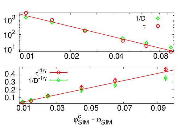
Rectification plots as shown in Fig. 23 corroborate that the asymtotic powerlaw holds for the collective relaxation time over at least two decades, and that a differing exponent or a different critical density would be required to render the diffusivity as a compatible MCT power law.

It is instructive to compare the wave-vector dependence of the relaxation times for the tagged-particle correlation function with the limiting behavior expected on hydrodynamic grounds, . To this end, we plot in Fig. 24 extracted from both the simulation and our MCT fits, at representative low and high packing fractions. Such plots have been suggested in discussing the non-Fickian transport evidenced by the van Hove functions shown above [63, 18]. There, has been defined as the point where the -dependent tagged-particle correlation function has decayed to . This quantity (open symbols and dashed lines in Fig. 24) approaches at low . At large it is expected to drop sharply: as the amplitude of the structural relaxation process, , drops below , the procedure no longer reliably probes slow relaxation, but rather is dominated by the microscopic short-time relaxation (essentially in a Brownian system, where ). A similar remark holds for the collective relaxation time ; the time-scale determined by the -criterion can only be compared to MCT as long as is sufficiently larger than .
Our findings for are in agreement with the Brownian dynamics simulations of Flenner and Szamel [18]: while MCT simply predicts a monotonic crossover between the two regimes, in the simulation data, an intermediate maximum at corresponding to the nearest-neighbor distance emerges as one approaches .
Since our MCT fits are matched to the collective correlation functions, a notable consequence in Fig. 24 is that for , MCT and simulation data for approach different constants, the MCT one being too high. This corroborates our interpretation that for the tagged-particle dynamics MCT is a reasonable theory for the intermediate and large wave numbers, and that deviations are increasingly seen as approaches zero. It differs from the interpretation of Ref. [18], where also simulation and MCT data for were compared, but normalized to their respective values. As a result, deviations were attributed mostly to the intermediate-, not the small- regime. In light of our results, it might be more suggestive to turn around the discussion: it is not the nearest-neighbor-scale modes that are unexpectedly slow, but it is the diffusion that is faster than expected from the MCT-embedded cage picture.

If one investigates the distinct part of the collective dynamics, i.e., density correlations that arise from distinct particles, MCT’s mis-description of tagged-particle dynamics has an interesting consequence. Recall that the distinct van Hove correlation function is given by the difference of collective and tagged-particle contributions, ; this means that within MCT, it is obtained from the inverse Fourier transform of . On physical grounds, must be a positive real function, since it measures the probability of finding a particle at time and distance from a distinct particle that was at the origin at . This property is not obvious from the difference formula.
Symbols in Fig. 25 show evaluated at various times covering the structural-relaxation regime for the simulations at the lowest and highest packing fraction we studied; we have normalized such that it approaches unity at long distances. We recover the expected shell structure that is inherited from the -th neighbor shells in the radial distribution function . These shells are increasingly washed out as time progresses, until the long-time limit is reached. Comparing with the MCT-calculated quantities (obtained from the fits in -space presented above), we note that at distances including and exceeding the nearest-neighbor distance, the MCT description is fairly good although not perfect. At small , however, there is a most obvious error as turns negative in the MCT approximation. Note that for small and for sufficiently large , this phenomenon does not occur, for trivial reasons; for small , the positiveness of within MCT hinges on that of , while for large , approaches the uniform density. Note that the positivity of may fail for approximate at some densities, but we have checked that this is not the case here.
The reason for the failure in the small- description is easily understood: both and are dominated by a strong peak centered on , since their values incorporate a -peak that is smeared out with time. Evaluating , we have to subtract these two large contributions from each other. In fact, for the plots shown, typical values of and are at the intermediate time, while . Numerically, this is a moderate error, which by looking at the distinct van Hove function is turned into a qualitative one. The error was in fact to be expected based on our discussion so far: the theory, by way of underestimating the single-particle diffusion coefficient, overestimates the localization of a tagged particle. This translates into a peak in that is to narrow and thus too high. Even if the description of the collective dynamics through were totally correct, this overestimation of single-particle localization is sufficient to render unphysically negative.
In the simulation data, one notices a subtle feature around that is, due to the reasons just outlined, outside the scope of MCT. At , raises from zero at short times to unity at long times. At the low density shown in Fig. 25, this filling in of the excluded-volume gap happens as naïvely expected from the broadening of the nearest-neighbor peak, resulting in functions that are always monotonically increasing with in the regime . At higher density, however, this monotonicity is lost, and an additional dip in evolves around . This qualitatively agrees with earlier findings from simulations of glass-forming binary mixtures [64, 65]. It is intuitively interpreted as the persistence of preferred interparticle distances: as a given particle moves away from its original position, there is an enhanced probability that another particle fills this position, rather than any nearby one.

It is worth noting that the issue of negative does not appear to be related to the dynamics. As shown in Fig. 26, the real-space representation of the nonergodicity parameters, calculated from the inverse Fourier transform of , shows the same features as discussed above. To ensure that no cutoff problems arise, we have based this quantity on the Percus-Yevick static structure factor with a wave-vector grid spacing and discretization points, and at packing fraction for one-component MCT. Note that we are still sufficiently far from the packing fraction where the PY- starts to be unphysical.
V Conclusion
We performed molecular-dynamics computer simulations of a polydisperse quasi-hard sphere system and analysed both the collective and the incoherent density-density correlation functions in the framework of both asymptotic predictions and full numerical solutions of the mode-coupling theory of the glass transition. For the latter, the required input in the form of static equilibrium structure factors has been also calculated from the MD simulation. To capture some essential effects of particle-size polydispersity in the MCT calculation, numerical solutions of one-, three-, and five-component systems with particle sizes chosen to match the first few moments of the true polydispersity distribution have been compared.
For the particular size distribution chosen in the simulation, the five-component analysis turned out to be mostly sufficient to capture the effects induced by a variation of particle size. These effects concern in particular the small-wave-number limit, , where mixtures of particles of unequal interactions (here: unequal sizes) show, even in the species-averaged correlation functions, signatures of interdiffusion processes that are well understood in principle in the framework of multicomponent hydrodynamics. MCT has this hydrodynamic limit built in, and consequently predicts a subtle interplay of the various interdiffusion modes with structural relaxation, leading at low to the appearance of double- peaks. These are less pronounced in the simulation, presumably due to them being smeared out in a truly polydisperse system, where the binning into a few number of components is not strictly meaningful.
Apart from the low- behavior, which however may be of significant interest as it determines the most commonly discussed transport coefficients, there is little difference between the different mixtures we considered. A general trend is that, taking the species average already on the level of static structure correlations, before entering MCT, is worse than performing this average only on the dynamic level. This is intuitively understood from the fact that such pre-averaging tends to smear out the correlations visible in the static structure factor as oscillations at large . For systems where the slow dynamics is driven by excluded-volume interactions, such as our quasi-hard-sphere system, this is a relatively minor quantitative effect. For systems where short-range interactions are crucial for the slow dynamics (affecting the large- tail of the structure functions), it will be even more crucial to treat polydisperse systems as mixtures rather than as effective-one-component systems.
Based on the simulation data and the known asymptotic results from MCT alone, we have first performed a traditional scaling analysis, revealing the coefficients involved in desribing the slow relaxation, and the -relaxation window at intermediate times. The coefficients, such as the plateau heights and critical amplitudes show good quantitative agreement with the corresponding quantities calculated within full MCT. A stretched-exponential relaxation analysis for the process reveals some mismatch in the stretching indices.
In fitting the full numerical MCT solutions to the data, only the relation between , the packing fraction entering the MCT vertex, and , the nominal packing fraction in the simulation, was adjusted, to absorb the well-known error in the numerical value of when calculated within full MCT. Indeed, the resulting relation can be very well described as linear with slope unity, so that effectively no fit parameter remains (or just one, if one accounts for the slope being slightly different from unity).
Basing this adjustment on the collective correlation functions for a single wave vector magnitude, , we obtain good agreement between MCT and the simulation data for the collective density correlators at essentially all sufficiently large . Deviations are most prominent where . At small , the one-component analysis shows severe deviations, in particular an order-of-magnitude mismatch in the relaxation time, attributed to the missing interdiffusion process discussed above. The three- and five-component MCT calculations do not suffer from this shortcoming and describe also the collective small- behavior reasonably well.
We have discussed the MCT description of the tagged-particle dynamics after all parameters have been fixed in the analysis of collective correlation functions. Here, the situation is more subtle: for exceeding roughly half the position of the structure-factor main peak, the MCT description is again reasonable. However, for , errors increase continuously, to become most prominent in an analysis of the mean-squared displacement (as has been noted in an earlier publication). Here, the MCT curves show a much stronger slowing down with increasing packing fraction, while the simulations exhibit averaged particle mobilities that are higher than those expected from either MCT or a Stokes-Einstein argument. This diffusion-relaxation decoupling is of course well known in the glass literature. The single-particle motion has been thoroughly investigated before in terms of van Hove functions, identifying subsets of fast and slow particles even in one-component systems [66]. Also in our system, such a splitting is observed. However, we wish to stress that it seems to affect mostly the MCT description of tagged-particle dynamics. At the same time, the MCT description of the collective density fluctuations remains remarkably accurate, and in particular the structural relaxation time extracted from the simulation does not show any significant deviation from the values predicted by the theory. For future work an analysis of the collective van Hove functions might provide additional information about the origin of these deviations.
We can of course not exclude the possibility that at even higher densities than those we could simulate, such deviations eventually set in. However, if this is the case, they need not coincide with the features typically discussed in terms of heterogeneous dynamics, viz. the decoupling of diffusivity from structural relaxation. It may be that our choice of a system driven by stochastic dynamics and without a significant energy scale in the particle interactions is fortuitous. However, this remains to be clarified. Within MCT, the independence of structural-relaxation properties of the time-evolution operator is a major result, confirmed before [30]. There are arguments that this correspondence does indeed extend also to the way simulation results deviate from MCT, but not to higher-order correlation functions such as four-point susceptibilities [67, 68].
It appears then that fitting incoherent correlation functions with MCT is a rather roundabout way of testing the theory, and that in particular it represents an unfortunate test (for the theory, at least) in that these quantities show strongest deviations from the predicted behavior. Unfortunately, the MSD is perhaps the quantity most often analyzed in simulation and in assessing MCT’s validity (since it is easy to compute with good statistics). Our analysis shows that it is the least valuable quantity to compare MCT with.
Our discussion suggests that other collective correlation functions provide a fruitful basis for further investigations of MCT and its approximations: in particular stress-stress auto-correlation functions should be analyzed, as they are cloesly linked to the memory kernel of the theory. However, these require even more computational effort to determine from simulation than the collective density correlators we have examined here: for the latter, we have averaged independent evaluations, while for the former, up to had to be used in previous work on a similar system with Newtonian dynamics [69].
Acknowledgements.
A.M.P. acknowledges financial support from the Spanish M.E.C. – project MAT2009-14234-CO3-02. Th.V. holds a Helmholtz-University Young Researcher Group fellowship (HGF VH-NG406), and is fellow of the Zukunftskolleg of the Universität Konstanz.References
- [1] U. Bengtzelius, W. Götze, and A. Sjölander, J. Phys. C 17, 5915 (1984).
- [2] E. Leutheusser, Phys. Rev. A 29, 2765 (1984).
- [3] W. Götze, J. Phys.: Condens. Matter 11, A1 (1999).
- [4] W. Götze, Complex Dynamics of Glass-Forming Liquids (Oxford University Press, Oxford, 2009).
- [5] W. Kob, J. Phys.: Condens. Matter 11, R89 (1999).
- [6] K. Binder and W. Kob, Glassy materials and disordered solids (World Scientific, Singapore, 2005).
- [7] W. Kob, C. Donati, S. J. Plimpton, P. H. Poole, and S. C. Glotzer, Phys. Rev. Lett. 79, 2827 (1997).
- [8] S. C. Glotzer, Y. Gebremichael, N. Lacevic, T. B. Schroder, and F. W. Starr, ACS Symposium Series 820, 214 (2002).
- [9] P. Pusey and W. van Megen, Nature 320, 340 (1986).
- [10] P. Pusey and W. van Megen, Physical Review Letters 59, 2083 (1987).
- [11] P. Pusey and W. V. Megen, Physica A: Statistical Mechanics and its Applications 157, 705 (1989), ISSN 0378-4371.
- [12] W. van Megen and S. M. Underwood, Phys. Rev. E 49, 4206 (1994).
- [13] W. van Megen, T. C. Mortensen, S. R. Williams, and J. Müller, Phys. Rev. E 58, 6073 (1998).
- [14] E. Flenner and G. Szamel, Phys. Rev. E 72, 011205 (2005a).
- [15] Th. Voigtmann, A. Meyer, D. Holland-Moritz, S. Süber, T. Hansen, and T. Unruh, EPL 82, 66001 (2008).
- [16] M. Nauroth and W. Kob, Phys. Rev. E 55, 657 (1997).
- [17] W. Kob, M. Nauroth, and F. Sciortino, J. Non-Cryst. Solids 307–310, 181 (2002).
- [18] E. Flenner and G. Szamel, Phys. Rev. E 72, 031508 (2005b).
- [19] G. Foffi, W. Götze, F. Sciortino, P. Tartaglia, and Th. Voigtmann, Phys. Rev. Lett. 91, 085701 (2003).
- [20] G. Foffi, W. Götze, F. Sciortino, P. Tartaglia, and Th. Voigtmann, Phys. Rev. E 69, 011505 (2004).
- [21] O. Henrich, A. M. Puertas, M. Sperl, J. Baschnagel, and M. Fuchs, Phys. Rev. E 76, 031404 (2007).
- [22] E. Zaccarelli, I. Saika-Voivod, A. J. Moreno, E. L. Nave, S. V. Buldyrev, F. Sciortino, and P. Tartaglia, Journal of Physics: Condensed Matter 18, S2373 (2006).
- [23] F. Sciortino and W. Kob, Phys. Rev. Lett. 86, 648 (2001).
- [24] Th. Voigtmann and J. Horbach, Europhys. Lett. 74, 459 (2006).
- [25] A. B. Mutiara and H. Teichler, Phys. Rev. E 64, 046133 (2001).
- [26] S.-H. Chong, M. Aichele, H. Meyer, M. Fuchs, and J. Baschnagel, Phys. Rev. E 76, 051806 (2007).
- [27] A. Rinaldi, F. Sciortino, and P. Tartaglia, Phys. Rev. E 63, 061210 (2001).
- [28] S.-H. Chong and F. Sciortino, Phys. Rev. E 69, 051202 (2004).
- [29] Th. Voigtmann, A. M. Puertas, and M. Fuchs, Phys. Rev. E 70, 061506 (2004).
- [30] T. Gleim and W. Kob, Eur. Phys. J. B 13, 83 (2000).
- [31] G. Szamel and E. Flenner, EPL (Europhysics Letters) 67, 779 (2004).
- [32] E. Lange, J. B. Caballero, A. M. Puertas, and M. Fuchs, J. Chem. Phys. 130, 174903 (2009).
- [33] S. R. Williams, C. P. Royall, and G. Bryant, Phys. Rev. Lett. 100, 225502 (2008).
- [34] E. Zaccarelli, C. Valeriani, E. Sanz, W. C. K. Poon, M. E. Cates, and P. N. Pusey, Phys. Rev. Lett. 103, 134704 (2009).
- [35] W. Götze, in Amorphous and Liquid Materials, edited by E. Lüscher, G. Fritsch, and G. Jacucci (Nijhoff Publishers, Dordrecht, 1987), NATO Advanced Study Institute Series E, pp. 34–81.
- [36] W. Götze and Th. Voigtmann, Phys. Rev. E 67, 021502 (2003).
- [37] J.-P. Hansen and I. R. McDonald, Theory of Simple Liquids (Academic Press, London, 1986), 2nd ed.
- [38] W. Paul and D. Y. Yoon, Phys. Rev. E 52, 2076 (1995).
- [39] P. J. Steinhardt, D. R. Nelson, and M. Ronchetti, Phys. Rev. B 28, 784 (1983).
- [40] P. R. ten Wolde, M. J. Ruiz-Montero, and D. Frenkel, J. Chem. Phys. 104, 9932 (1996).
- [41] W. Götze, in Liquids, Freezing and Glass Transition, edited by J.-P. Hansen, D. Levesque, and J. Zinn-Justin (North-Holland, Amsterdam, 1991), Les Houches Summer Schools of Theoretical Physics, pp. 287–503.
- [42] T. Franosch, M. Fuchs, W. Götze, M. R. Mayr, and A. P. Singh, Phys. Rev. E 55, 7153 (1997).
- [43] M. Fuchs, W. Götze, and M. R. Mayr, Phys. Rev. E 58, 3384 (1998).
- [44] W. Götze and L. Sjögren, J. Math. Analysis Appl. 195, 230 (1995).
- [45] T. Franosch and Th. Voigtmann, J. Stat. Phys. 109, 237 (2002).
- [46] M. S. Wertheim, Phys. Rev. Lett. 10, 321 (1963).
- [47] W. van Megen and S. M. Underwood, Phys. Rev. Lett. 70, 2766 (1993).
- [48] F. N. Braun and J. Bergenholtz, J. Chem. Phys. B 111, 11626 (2007).
- [49] M. Fuchs, J. Non-Cryst. Solids 172–174, 241 (1994).
- [50] F. Sciortino and P. Tartaglia, J. Chem. Phys. 11, A261 (1999), ISSN 0953-8984.
- [51] M. Fuchs and A. Latz, Physica A 201, 1 (1993).
- [52] F. Weysser (2007), Diplomarbeit, Universität Konstanz.
- [53] O. Gräser (2006), Diplomarbeit, Universität Konstanz.
- [54] G. Brambilla, D. El Masri, M. Pierno, L. Berthier, L. Cipelletti, G. Petekidis, and A. B. Schofield, Phys. Rev. Lett. 102, 085703 (2009).
- [55] C. G. Small, Int. Stat. Rev. 56, 243 (1988).
- [56] W. Kob, in Slow Relaxations and Nonequilibrium Dynamics in Condensed Matter, edited by J.-L. Barrat, M. Feigelman, J. Kurchan, and J. Dalibard (Springer, Berlin, 2003), vol. Session LXXVII (2002) of Les Houches Summer Schools of Theoretical Physics, pp. 199–269.
- [57] M. Sperl, Phys. Rev. E 71, 060401 (2005).
- [58] W. van Megen, Phys. Rev. E 76, 061401 (2007).
- [59] M. E. Cates, M. Fuchs, K. Kroy, W. C. K. Poon, and A. M. Puertas, J. Phys.: Condens. Matter 16, S4861 (2004).
- [60] A. M. Puertas, M. Fuchs, and M. E. Cates, J. Chem. Phys. 121, 2813 (2004).
- [61] D. R. Reichmann, E. Rabani, and P. L. Geissler, J. Chem. Phys. 109, 14654 (2005).
- [62] G. Szamel and E. Flenner, Phys. Rev. E 73, 011504 (2006a).
- [63] L. Berthier, Phys. Rev. E 69, 020201(R) (2004).
- [64] W. Kob and H. C. Andersen, Phys. Rev. E 51, 4626 (1995).
- [65] S. Sanyal and A. K. Sood, Phys. Rev. E 57, 908 (1998).
- [66] S. K. Kumar, G. Szamel, and J. F. Douglas, J. Chem. Phys. 124, 214501 (2006).
- [67] G. Szamel and E. Flenner, Phys. Rev. E 74, 021507 (2006b).
- [68] L. Berthier and W. Kob, J. Phys.: Condens. Matter 19, 205130 (2007).
- [69] A. M. Puertas, C. De Michele, F. Sciortino, P. Tartaglia, and E. Zaccarelli, J. Chem. Phys. 127, 144906 (2007).