跳到论文正文
W Papers独立论文阅读器 arXiv:1003.3722 论文正文 计算阅读时间 · 0%
引用这篇论文根据当前论文元数据生成,正式投稿前建议核对。


License: arXiv.org perpetual non-exclusive license
arXiv:1003.3722v1 [math.PR] 19 Mar 2010

Stochastic domination for the Ising and fuzzy Potts modelsThanks: Research partially supported by the Göran Gustafsson Foundation for Research in Natural Sciences and Medicine.

Marcus Warfheimer Address: Department of Mathematical Sciences, Chalmers University of Technology and University of Gothenburg, SE–41296 Gothenburg, Sweden Email address: marcus.warfheimer@gmail.com URL: http://www.math.chalmers.se/˜warfheim
Date: August 24, 2026
Abstract.

We discuss various aspects concerning stochastic domination for the Ising model and the fuzzy Potts model. We begin by considering the Ising model on the homogeneous tree of degree dd, 𝕋d{\mathbb{T}}^{d}. For given interaction parameters J1J_{1}, J2>0J_{2}>0 and external field h1∈ℝh_{1}\in{\mathbb{R}}, we compute the smallest external field h~\tilde{h} such that the plus measure with parameters J2J_{2} and hh dominates the plus measure with parameters J1J_{1} and h1h_{1} for all h≥h~h\geq\tilde{h}. Moreover, we discuss continuity of h~\tilde{h} with respect to the three parameters J1J_{1}, J2J_{2}, hh and also how the plus measures are stochastically ordered in the interaction parameter for a fixed external field. Next, we consider the fuzzy Potts model and prove that on ℤd{\mathbb{Z}}^{d} the fuzzy Potts measures dominate the same set of product measures while on 𝕋d{\mathbb{T}}^{d}, for certain parameter values, the free and minus fuzzy Potts measures dominate different product measures. For the Ising model, Liggett and Steif proved that on ℤd{\mathbb{Z}}^{d} the plus measures dominate the same set of product measures while on 𝕋2{\mathbb{T}}^{2} that statement fails completely except when there is a unique phase.

Key words and phrases: 
Stochastic domination, Ising model, fuzzy Potts model, domination of product measures
2000 Mathematics Subject Classification
60K35

1. Introduction and main results

The concept of stochastic domination has played an important role in probability theory over the last couple of decades, for example in interacting particle systems and statistical mechanics. In [13], various results were proved concerning stochastic domination for the Ising model with no external field on ℤd{\mathbb{Z}}^{d} and on the homogeneous binary tree 𝕋2{\mathbb{T}}^{2} (i.e. the unique infinite tree where each site has 33 neighbors). As an example, the following distinction between ℤd{\mathbb{Z}}^{d} and 𝕋2{\mathbb{T}}^{2} was shown: On ℤd{\mathbb{Z}}^{d}, the plus and minus states dominate the same set of product measures, while on 𝕋2{\mathbb{T}}^{2} that statement fails completely except in the case when we have a unique phase. In this paper we study stochastic domination for the Ising model in the case of nonzero external field and also for the so called fuzzy Potts model.

Let VV be a finite or countable set and equip the space {−1,1}V\{-1,1\}^{V} with the following natural partial order: For η\eta, η′∈{−1,1}V\eta^{\prime}\in\{-1,1\}^{V}, we write η≤η′\eta\leq\eta^{\prime} if η⁡(x)≤η′​(x)\eta(x)\leq\eta^{\prime}(x) for all x∈Vx\in V. Moreover, whenever we need a topology on {−1,1}V\{-1,1\}^{V} we will use the product topology. We say that a function f:{−1,1}V→ℝf:\{-1,1\}^{V}\to{\mathbb{R}} is increasing if f⁡(η)≤f⁡(η′)f(\eta)\leq f(\eta^{\prime}) whenever η≤η′\eta\leq\eta^{\prime}. We will use the following usual definition of stochastic domination.

Definition 1.1 (Stochastic domination).

Given a finite or countable set VV and probability measures μ1\mu_{1}, μ2\mu_{2} on {−1,1}V\{-1,1\}^{V}, we say that μ2\mu_{2} dominates μ1\mu_{1} (written μ1≤μ2\mu_{1}\leq\mu_{2} or μ2≥μ1\mu_{2}\geq\mu_{1}) if

∫f​d​μ1≤∫f​d​μ2\int f\,d\mu_{1}\leq\int f\,d\mu_{2}

for all real-valued, continuous and increasing functions ff on {−1,1}V\{-1,1\}^{V}.

It is well known that a necessary and sufficient condition for two probability measures μ1\mu_{1}, μ2\mu_{2} to satisfy μ1≤μ2\mu_{1}\leq\mu_{2} is that there exists a coupling measure ν\nu on {−1,1}V×{−1,1}V\{-1,1\}^{V}\times\{-1,1\}^{V} with first and second marginals equal to μ1\mu_{1} and μ2\mu_{2} respectively and

ν((η,ξ):η≤ξ)=1.\nu(\,(\eta,\xi):\eta\leq\xi\,)=1.

(For a proof, see for example [12, p. 72-74].) Given any set S⊆ℝS\subseteq{\mathbb{R}} and a family of probability measures {μs}s∈S\{\mu_{s}\}_{s\in S} indexed by SS, we will say that the map S∋s↦μsS\ni s\mapsto\mu_{s} is increasing if μs1≤μs2\mu_{s_{1}}\leq\mu_{s_{2}} whenever s1<s2s_{1}<s_{2}.

1.1. The Ising model

The ferromagnetic Ising model is a well studied object in both physics and probability theory. For a given infinite, locally finite (i.e. each vertex has a finite number of neighbors), connected graph G=(V,E)G=(V,E), it is defined from the nearest-neighbor potential

ΦAJ,h​(η)={−J​η​(x)​η​(y)if A={x,y}, with ⟨x,y⟩∈E,−h​η​(x)if A={x},0otherwise\Phi_{A}^{J,h}(\eta)=\begin{cases}-J\eta(x)\eta(y)&\text{if $A=\{x,y\}$, with $\langle x,y\rangle\in E$},\\ -h\eta(x)&\text{if $A=\{x\}$},\\ 0&\text{otherwise}\end{cases}

where A⊆VA\subseteq V, η∈{−1,1}V\eta\in\{-1,1\}^{V}, J>0J>0, h∈ℝh\in{\mathbb{R}} are two parameters called the coupling strength and the external field respectively and ⟨x,y⟩\langle x,y\rangle denotes the edge connecting xx and yy. A probability measure μ\mu on {−1,1}V\{-1,1\}^{V} is said to be a Gibbs measure (or sometimes Gibbs state) for the ferromagnetic Ising model with parameters h∈ℝh\in{\mathbb{R}} and J>0J>0 if it admits conditional probabilities such that for all finite U⊆VU\subseteq V, all σ∈{−1,1}U\sigma\in\{-1,1\}^{U} and all η∈{−1,1}V∖U\eta\in\{-1,1\}^{V\setminus U}

μ⁡(X⁡(U)=σ|X⁡(V∖U)=η)\displaystyle\mu(X(U)=\sigma\,|\,X(V\setminus U)=\eta)
=1ZJ,hU,ηexp[J(∑⟨x,y⟩∈E,x,y∈Uσ(x)σ(y)+∑⟨x,y⟩∈E,x∈U,y∈∂Uσ(x)η(y))\displaystyle\quad=\frac{1}{Z_{J,h}^{U,\eta}}\exp\Bigg[J\Bigg(\displaystyle\sum_{\langle x,y\rangle\in E,x,y\in U}\sigma(x)\sigma(y)+\sum_{\langle x,y\rangle\in E,x\in U,y\in\partial U}\sigma(x)\eta(y)\Bigg)
+h∑x∈Uσ(x)]\displaystyle\qquad+h\sum_{x\in U}\sigma(x)\Bigg]

where ZJ,hU,ηZ_{J,h}^{U,\eta} is a normalizing constant and

∂U={x∈V∖U:∃y∈U​ such that ​⟨x,y⟩∈E}.\partial U=\{\,x\in V\setminus U:\exists y\in U\text{ such that }\langle x,y\rangle\in E\,\}.

For given J>0J>0 and h∈ℝh\in{\mathbb{R}}, we will denote the set of Gibbs measures with parameters JJ and hh by 𝒢⁡(J,h)\mathcal{G}(J,h) and we say that a phase transition occurs if |𝒢⁡(J,h)|>1|\mathcal{G}(J,h)|>1, i.e. if there exist more than one Gibbs state. (From the general theory described in [2] or [12], 𝒢⁡(J,h)\mathcal{G}(J,h) is always nonempty.) At this stage one can ask, for fixed h∈ℝh\in{\mathbb{R}}, is it the case that the existence of multiple Gibbs states is increasing in JJ? When h=0h=0 it is possible from the so called random-cluster representation of the Ising model to show a positive answer to the last question (see [5] for the case when G=ℤdG={\mathbb{Z}}^{d} and [7] for more general GG). However, when h≠0h\neq 0 there are graphs where the above monontonicity property no longer holds, see [15] for an example of a relatively simple such graph.

Furthermore, still for fixed J>0J>0, h∈ℝh\in{\mathbb{R}}, standard monotonicity arguments can be used to show that there exists two particular Gibbs states μhJ,+\mu_{h}^{J,+}, μhJ,−\mu_{h}^{J,-}, called the plus and the minus state, which are extreme with respect to the stochastic ordering in the sense that

(1.1) μhJ,−≤μ≤μhJ,+for any other μ∈𝒢⁡(J,h).\mu_{h}^{J,-}\leq\mu\leq\mu_{h}^{J,+}\quad\text{for any other $\mu\in\mathcal{G}(J,h)$}.

To simplify the notation, we will write μJ,+\mu^{J,+} for μ0J,+\mu_{0}^{J,+} and μJ,−\mu^{J,-} for μ0J,−\mu_{0}^{J,-}. (Of course, most of the things we have defined so far are also highly dependent on the graph GG, but we suppress that in the notation.)

In [13] the authors studied, among other things, stochastic domination between the plus measures {μJ,+}J>0\{\mu^{J,+}\}_{J>0} in the case when G=𝕋2G={\mathbb{T}}^{2}. For example they showed that the map (0,∞)∋J↦μJ,+(0,\infty)\ni J\mapsto\mu^{J,+} is increasing when J>JcJ>J_{c} and proved the existence of and computed the smallest J>JcJ>J_{c} such that μJ,+\mu^{J,+} dominates μJ′,+\mu^{J^{\prime},+} for all 0<J′≤Jc0<J^{\prime}\leq J_{c}. (On ℤd{\mathbb{Z}}^{d}, the fact that μJ1,+\mu^{J_{1},+} and μJ2,+\mu^{J_{2},+} are not stochastically ordered when J1≠J2J_{1}\neq J_{2} gives that such a JJ does not even exist in that case.) Our first result deals with the following question: Given J1J_{1}, J2>0J_{2}>0, h1∈ℝh_{1}\in{\mathbb{R}}, can we find the smallest external field h~=h~​(J1,J2,h1)\tilde{h}=\tilde{h}(J_{1},J_{2},h_{1}) with the property that μhJ2,+\mu_{h}^{J_{2},+} dominates μh1J1,+\mu_{h_{1}}^{J_{1},+} for all h≥h~h\geq\tilde{h}? To clarify the question a bit more, note that an easy application of Holley’s theorem (see [3]) tells us that for fixed J>0J>0, the map ℝ∋h↦μhJ,+{\mathbb{R}}\ni h\mapsto\mu_{h}^{J,+} is increasing. Hence, for given J1J_{1}, J2J_{2} and h1h_{1} as above the set

{h∈ℝ:μhJ2,+≥μh1J1,±}\{\,h\in{\mathbb{R}}:\mu_{h}^{J_{2},+}\geq\mu_{h_{1}}^{J_{1},\pm}\,\}

is an infinite interval and we want to find the left endpoint of that interval (possibly −∞-\infty or +∞+\infty at this stage). For a general graph not much can be said, but we have the following easy bounds on h~\tilde{h} when GG is of bounded degree.

Proposition 1.1.

Consider the Ising model on a general graph G=(V,E)G=(V,E) of bounded degree. Define

h~=h~​(J1,J2,h1)=inf{h∈ℝ:μhJ2,+≥μh1J1,+}.\tilde{h}=\tilde{h}(J_{1},J_{2},h_{1})=\inf\{\,h\in{\mathbb{R}}:\,\mu_{h}^{J_{2},+}\geq\mu_{h_{1}}^{J_{1},+}\,\}.

Then

h1−N⁡(J1+J2)≤h~≤h1+N​|J1−J2|,h_{1}-N(J_{1}+J_{2})\leq\tilde{h}\leq h_{1}+N|J_{1}-J_{2}|,

where N=supx∈VNxN=\displaystyle\sup_{x\in V}N_{x} and NxN_{x} is the number of neighbors of the site x∈Vx\in V.

For the Ising model, we will now consider the case when G=𝕋dG={\mathbb{T}}^{d}, the homogeneous dd-ary tree, defined as the unique infinite tree where each site has exactly d+1≥3d+1\geq 3 neighbors. The parameter dd is fixed in all that we will do and so we suppress that in the notation. For this particular graph it is well known that for given h∈ℝh\in{\mathbb{R}}, the existence of multiple Gibbs states is increasing in JJ and so as a consequence there exists a critical value Jc​(h)∈[0,∞]J_{c}(h)\in[0,\infty] such that when J<Jc​(h)J<J_{c}(h) we have a unique Gibbs state whereas for J>Jc​(h)J>J_{c}(h) there are more than one Gibbs states. In fact, much more can be shown in this case. As an example it is possible to derive an explicit expression for the phase transition region

{(J,h)∈ℝ2:|𝒢⁡(J,h)|>1},\{\,(J,h)\in{\mathbb{R}}^{2}:\,|\mathcal{G}(J,h)|>1\,\},

in particular one can see that Jc​(h)∈(0,∞)J_{c}(h)\in(0,\infty) for all h∈ℝh\in{\mathbb{R}}. Moreover,

Jc:=Jc​(0)=arccoth ​d=12​log⁡d+1d−1,J_{c}:=J_{c}(0)=\text{arccoth }\,{}^{\!\!}d=\frac{1}{2}\log\frac{d+1}{d-1},

see [2] for more details. (Here and in the sequel, :⁣=:= will mean definition.)

To state our results for the Ising model on 𝕋d{\mathbb{T}}^{d}, we need to recall some more facts, all of which can be found in [2, p. 247-255]. To begin, we just state what we need very briefly and later on we will give some more details. Given J>0J>0 and h∈ℝh\in{\mathbb{R}}, there is a one-to-one correspondence t↦μt\mapsto\mu between the real solutions of a certain equation (see (2.3) and the function ϕJ\phi_{J} in (2.2) below) and the completely homogeneous Markov chains in 𝒢⁡(J,h)\mathcal{G}(J,h) (to be defined in Section 2). Let t±​(J,h)t_{\pm}(J,h) denote the real numbers which correspond to the plus and minus measure respectively. (It is easy to see that the plus and minus states are completely homogeneous Markov chains, see Section 2.) We will write t±​(J)t_{\pm}(J) instead of t±​(J,0)t_{\pm}(J,0). Furthermore, let

h∗​(J)=maxt≥0⁡(d​ϕJ​(t)−t)h^{*}(J)=\displaystyle\max_{t\geq 0}\big(d{}^{\,\,}\!\phi_{J}(t)-t\big)

and denote by t∗​(J)t^{*}(J) the t≥0t\geq 0 where the function t↦d​ϕJ​(t)−tt\mapsto d{}^{\,\,}\!\phi_{J}(t)-t attains its unique maximum. In [2], explicit expressions for both h∗h^{*} and t∗t^{*} are derived:

h∗​(J)={0if J≤Jcd​arctanh​(d​tanh⁡(J)−1d​coth⁡(J)−1)1/2−arctanh​(d−coth⁡(J)d−tanh⁡(J))1/2if J>Jc\displaystyle h^{*}(J)=\begin{cases}0\quad&\text{if $J\leq J_{c}$}\\ d{}^{\,\,}\!\text{arctanh}\left(\frac{d\tanh(J)-1}{d\coth(J)-1}\right)^{1/2}-\text{arctanh}\left(\frac{d-\coth(J)}{d-\tanh(J)}\right)^{1/2}\quad&\text{if $J>J_{c}$}\end{cases}
t∗​(J)={0if J≤Jcarctanh​(d−coth⁡(J)d−tanh⁡(J))1/2if J>Jc\displaystyle t^{*}(J)=\begin{cases}0\quad&\text{if $J\leq J_{c}$}\\ \text{arctanh}\left(\frac{d-\coth(J)}{d-\tanh(J)}\right)^{1/2}\quad&\text{if $J>J_{c}$}\end{cases}

In particular one can see that both h∗h^{*} and t∗t^{*} are continuous functions of JJ and by computing derivatives one can show that they are strictly increasing for J>JcJ>J_{c}.

Refer to caption
Figure 1.1. The functions h∗h^{*} and t∗t^{*} in the case when d=4d=4.
Theorem 1.2.

Consider the Ising model on 𝕋d{\mathbb{T}}^{d} and let J1J_{1}, J2>0J_{2}>0, h1∈ℝh_{1}\in{\mathbb{R}} be given. Define

f±​(J1,J2,h1)\displaystyle f_{\pm}(J_{1},J_{2},h_{1}) =inf{h∈ℝ:μhJ2,+≥μh1J1,±}\displaystyle=\inf\{\,h\in{\mathbb{R}}:\mu_{h}^{J_{2},+}\geq\mu_{h_{1}}^{J_{1},\pm}\,\}
g±​(J1,J2,h1)\displaystyle g_{\pm}(J_{1},J_{2},h_{1}) =inf{h∈ℝ:μhJ2,−≥μh1J1,±}\displaystyle=\inf\{\,h\in{\mathbb{R}}:\mu_{h}^{J_{2},-}\geq\mu_{h_{1}}^{J_{1},\pm}\,\}

and denote τ±=τ±​(J1,J2,h1)=t±​(J1,h1)+|J1−J2|\tau_{\pm}=\tau_{\pm}(J_{1},J_{2},h_{1})=t_{\pm}(J_{1},h_{1})+|J_{1}-J_{2}|. Then the following holds:

(1.2) f±​(J1,J2,h1)={−h∗​(J2)if ​t−​(J2,−h∗​(J2))≤τ±<t∗​(J2)τ±−d​ϕJ2​(τ±)if ​τ±≥t∗​(J2)​ or ​τ±<t−​(J2,−h∗​(J2))f_{\pm}(J_{1},J_{2},h_{1})=\begin{cases}-h^{*}(J_{2})&\text{if }t_{-}(J_{2},-h^{*}(J_{2}))\leq\tau_{\pm}<t^{*}(J_{2})\\ \tau_{\pm}-d{}^{\,\,}\!\phi_{J_{2}}(\tau_{\pm})&\text{if }\tau_{\pm}\geq t^{*}(J_{2})\text{ or }\tau_{\pm}<t_{-}(J_{2},-h^{*}(J_{2}))\end{cases}
(1.3) g±​(J1,J2,h1)={h∗​(J2)if −t∗​(J2)<τ±≤t+​(J2,h∗​(J2))τ±−d​ϕJ2​(τ±)if ​τ±≤−t∗​(J2)​ or ​τ±>t+​(J2,h∗​(J2))g_{\pm}(J_{1},J_{2},h_{1})=\begin{cases}h^{*}(J_{2})&\text{if }-t^{*}(J_{2})<\tau_{\pm}\leq t_{+}(J_{2},h^{*}(J_{2}))\\ \tau_{\pm}-d{}^{\,\,}\!\phi_{J_{2}}(\tau_{\pm})&\text{if }\tau_{\pm}\leq-t^{*}(J_{2})\text{ or }\tau_{\pm}>t_{+}(J_{2},h^{*}(J_{2}))\end{cases}

Remarks.

  • (i)

    Note that if 0<J2≤Jc0<J_{2}\leq J_{c}, then h∗​(J2)=0h^{*}(J_{2})=0 and

    t−​(J2,−h∗​(J2))=t∗​(J2)=t+​(J2,h∗​(J2))=0t_{-}(J_{2},-h^{*}(J_{2}))=t^{*}(J_{2})=t_{+}(J_{2},h^{*}(J_{2}))=0

    and hence the first interval disappears in the formulas and we simply get

    f±​(J1,J2,h1)=g±​(J1,J2,h1)=τ±​(J1,J2,h1)−d​ϕJ2​(τ±​(J1,J2,h1)).\begin{split}f_{\pm}(J_{1},J_{2},h_{1})&=g_{\pm}(J_{1},J_{2},h_{1})\\ &=\tau_{\pm}(J_{1},J_{2},h_{1})-d\phi_{J_{2}}(\tau_{\pm}(J_{1},J_{2},h_{1})).\end{split}
  • (ii)

    By looking at the formulas (1.2) and (1.3), we see that there are functions ψ\psi, θ:(0,∞)×ℝ↦ℝ\theta:(0,\infty)\times{\mathbb{R}}\mapsto{\mathbb{R}} such that

    f±​(J1,J2,h1)=ψ(J2,τ±(J1,J2,h1))andg±​(J1,J2,h1)=θ⁡(J2,τ±​(J1,J2,h1)).\begin{split}f_{\pm}(J_{1},J_{2},h_{1})&=\psi(J_{2},\tau_{\pm}(J_{1},J_{2},h_{1}))\quad\text{and}\\ g_{\pm}(J_{1},J_{2},h_{1})&=\theta(J_{2},\tau_{\pm}(J_{1},J_{2},h_{1})).\end{split}

    (Of course, ψ⁡(J2,t)\psi(J_{2},t) and θ⁡(J2,t)\theta(J_{2},t) are just (1.2) and (1.3) with tt instead of τ±\tau_{\pm}.) It is easy to check that for fixed J2>0J_{2}>0, the maps t↦ψ⁡(J2,t)t\mapsto\psi(J_{2},t) and t↦θ⁡(J2,t)t\mapsto\theta(J_{2},t) are continuous. A picture of these functions when J2=2J_{2}=2, d=4d=4 can be seen in Figure 1.2.

  • (iii)

    It is not hard to see by direct computations that f+f_{+} satisfies the bounds in Proposition 1.1. We will indicate how this can be done after the proof of Theorem 1.2.

  • (iv)

    We will see in the proof that if

    t−​(J2,−h∗​(J2))≤τ±​(J1,J2,h1)<t∗​(J2),t_{-}(J_{2},-h^{*}(J_{2}))\leq\tau_{\pm}(J_{1},J_{2},h_{1})<t^{*}(J_{2}),

    then

    {h∈ℝ:μhJ2,+≥μh1J1,±}=[−h∗(J2),∞),\{\,h\in{\mathbb{R}}:\mu_{h}^{J_{2},+}\geq\mu_{h_{1}}^{J_{1},\pm}\,\}=[-h^{*}(J_{2}),\infty),

    and if −t∗​(J2)<τ±​(J1,J2,h1)≤t+​(J2,h∗​(J2))-t^{*}(J_{2})<\tau_{\pm}(J_{1},J_{2},h_{1})\leq t_{+}(J_{2},h^{*}(J_{2})), then

    {h∈ℝ:μhJ2,−≥μh1J1,±}=(h∗​(J2),∞).\{\,h\in{\mathbb{R}}:\mu_{h}^{J_{2},-}\geq\mu_{h_{1}}^{J_{1},\pm}\,\}=(h^{*}(J_{2}),\infty).

    Hence in the first case the left endpoint belongs to the interval, while in the second case it does not.
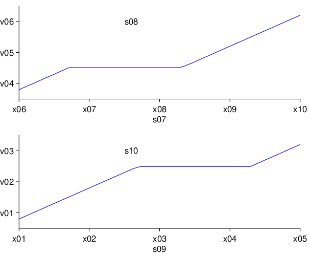
Refer to caption
Figure 1.2. The functions t↦ψ⁡(J2,t)t\mapsto\psi(J_{2},t) and t↦θ⁡(J2,t)t\mapsto\theta(J_{2},t) in the case when J2=2J_{2}=2 and d=4d=4.

Our next proposition deals with continuity properties of f±f_{\pm} and g±g_{\pm} with respect to the parameters J1J_{1}, J2J_{2} and h1h_{1}. We will only discuss the function f+f_{+}, the other ones can be treated in a similar fashion.

Proposition 1.3.

Consider the Ising model on 𝕋d{\mathbb{T}}^{d} and recall the notation from Theorem 1.2. Let

a=a⁡(J1,J2)\displaystyle a=a(J_{1},J_{2}) =t−​(J1,−h∗​(J1))+|J1−J2|\displaystyle=t_{-}(J_{1},-h^{*}(J_{1}))+|J_{1}-J_{2}|
b=b⁡(J1,J2)\displaystyle b=b(J_{1},J_{2}) =t+​(J1,−h∗​(J1))+|J1−J2|\displaystyle=t_{+}(J_{1},-h^{*}(J_{1}))+|J_{1}-J_{2}|
  • a)

    Given J1J_{1}, J2>0J_{2}>0, the map ℝ∋h1↦f+​(J1,J2,h1){\mathbb{R}}\ni h_{1}\mapsto f_{+}(J_{1},J_{2},h_{1}) is continuous except possibly at −h∗​(J1)-h^{*}(J_{1}) depending on J1J_{1} and J2J_{2} in the following way:

    • If J1≤JcJ_{1}\leq J_{c} or J1=J2J_{1}=J_{2} then it is continuous at −h∗​(J1)-h^{*}(J_{1}).

    • If J1>JcJ_{1}>J_{c} and 0<J2≤Jc0<J_{2}\leq J_{c} then it is discontinuous at −h∗​(J1)-h^{*}(J_{1}).

    • If J1J_{1}, J2>JcJ_{2}>J_{c}, J1≠J2J_{1}\neq J_{2} then it is discontinuous except when

      t−​(J2,−h∗​(J2))≤a<t∗​(J2)​and​t−​(J2,−h∗​(J2))≤b≤t∗​(J2).t_{-}(J_{2},-h^{*}(J_{2}))\leq a<t^{*}(J_{2})\;\,\text{and}\;\,t_{-}(J_{2},-h^{*}(J_{2}))\leq b\leq t^{*}(J_{2}).
  • b)

    Given J2>0J_{2}>0, h1∈ℝh_{1}\in{\mathbb{R}}, the map (0,∞)∋J1↦f+​(J1,J2,h1)(0,\infty)\ni J_{1}\mapsto f_{+}(J_{1},J_{2},h_{1}) is continuous at J1J_{1} if 0<J1≤Jc0<J_{1}\leq J_{c} or J1>JcJ_{1}>J_{c} and h1≠−h∗​(J1)h_{1}\neq-h^{*}(J_{1}). In the case when h1=−h∗​(J1)h_{1}=-h^{*}(J_{1}) it is discontinuous at J1J_{1} except when

    t−​(J2,−h∗​(J2))≤a<t∗​(J2)​and​t−​(J2,−h∗​(J2))≤b≤t∗​(J2).t_{-}(J_{2},-h^{*}(J_{2}))\leq a<t^{*}(J_{2})\;\,\text{and}\;\,t_{-}(J_{2},-h^{*}(J_{2}))\leq b\leq t^{*}(J_{2}).
  • c)

    Given J1>0J_{1}>0, h1∈ℝh_{1}\in{\mathbb{R}}, the map (0,∞)∋J2↦f+​(J1,J2,h1)(0,\infty)\ni J_{2}\mapsto f_{+}(J_{1},J_{2},h_{1}) is continuous for all J2>0J_{2}>0.

We conclude this section with a result about how the measures {μhJ,+}J>0\{\mu_{h}^{J,+}\}_{J>0} are ordered with respect to JJ for fixed h∈ℝh\in{\mathbb{R}}.

Proposition 1.4.

Consider the Ising model on 𝕋d{\mathbb{T}}^{d}. The map (0,∞)∋J↦μhJ,+(0,\infty)\ni J\mapsto\mu_{h}^{J,+} is increasing in the following cases: 𝑂𝑃𝐸𝑁a)a) h≥0h\geq 0 and J≥JcJ\geq J_{c}, 𝑂𝑃𝐸𝑁b)b) h<0h<0 and h∗​(J)>−hh^{*}(J)>-h.

1.2. The fuzzy Potts model

Next, we consider the so called fuzzy Potts model. To define the model, we first need to define the perhaps more familiar Potts model. Let G=(V,E)G=(V,E) be an infinite locally finite graph and suppose that q≥3q\geq 3 is an integer. Let UU be a finite subset of VV and consider the finite graph HH with vertex set UU and edge set consisting of those edges ⟨x,y⟩∈E\langle x,y\rangle\in E with x,y∈Ux,y\in U. In this way, we say that the graph HH is induced by UU. The finite volume Gibbs measure for the qq-state Potts model at inverse temperature J≥0J\geq 0 with free boundary condition is defined to be the probability measure πq,JH\pi_{q,J}^{H} on {1,2,…,q}U\{1,2,\dots,q\}^{U} which to each element σ\sigma assigns probability

πq,JH(σ)=1Zq,JHexp(2J∑⟨x,y⟩∈E,x,y∈UI{σ(x)=σ(y)}),\pi_{q,J}^{H}(\sigma)=\frac{1}{Z_{q,J}^{H}}\exp\bigg(2J\sum_{\langle x,y\rangle\in E,x,y\in U}I_{\{\sigma(x)=\sigma(y)\}}\bigg),

where Zq,JHZ_{q,J}^{H} is a normalizing constant.

Now, suppose r∈{1,…,q−1}r\in\{1,\dots,q-1\} and pick a πq,JH\pi_{q,J}^{H}\,- distributed object XX and for x∈Ux\in U let

(1.4) Y⁡(x)={−1 if ​X​(x)∈{1,…,r}1 if ​X​(x)∈{r+1,…,q}.Y(x)=\begin{cases}-1&\text{ if }X(x)\in\{1,\dots,r\}\\ \>\>{}^{\,\,}\!{}^{\,\,}\!{}^{\,\,}\!1&\text{ if }X(x)\in\{r+1,\dots,q\}.\end{cases}

We write νq,J,rH\nu_{q,J,r}^{H} for the resulting probability measure on {−1,1}U\{-1,1\}^{U} and call it the finite volume fuzzy Potts measure on HH with free boundary condition and parameters qq, JJ and rr.

We also need to consider the case when we have a boundary condition. For finite U⊆VU\subseteq V, consider the graph HH induced by the vertex set U∪∂UU\cup\partial U and let η∈{1,…,q}V∖U\eta\in\{1,\dots,q\}^{V\setminus U}. The finite volume Gibbs measure for the qq-state Potts model at inverse temperature J≥0J\geq 0 with boundary condition η\eta is defined to be the probability measure on {1,…,q}U\{1,\dots,q\}^{U} which to each element assigns probability

πq,JH,η​(σ)=1Zq,JH,ηexp(2J∑⟨x,y⟩∈E,x,y∈UI{σ(x)=σ(y)}+2J∑⟨x,y⟩∈E,x∈U,y∈∂UI{σ(x)=η(y)}),\begin{split}\pi_{q,J}^{H,\eta}(\sigma)&=\frac{1}{Z_{q,J}^{H,\eta}}\exp\Bigg(2J\displaystyle\sum_{\langle x,y\rangle\in E,x,y\in U}I_{\{\sigma(x)=\sigma(y)\}}\\ &\quad+2J\sum_{\langle x,y\rangle\in E,x\in U,y\in\partial U}I_{\{\sigma(x)=\eta(y)\}}\Bigg),\end{split}

where Zq,JH,ηZ_{q,J}^{H,\eta} is a normalizing constant. In the case when η≡i\eta\equiv i for some i∈{1,…,q}i\in\{1,\dots,q\}, we replace η\eta with ii in the notation.

Furthermore, we introduce the notion of infinite volume Gibbs measure for the Potts model. A probability measure μ\mu on {1,…,q}V\{1,\dots,q\}^{V} is said to be an infinite volume Gibbs measure for the qq-state Potts model on GG at inverse temperature J≥0J\geq 0, if it admits conditional probabilities such that for all finite U⊆VU\subseteq V, all σ∈{1,…,q}U\sigma\in\{1,\dots,q\}^{U} and all η∈{1,…,q}V∖U\eta\in\{1,\dots,q\}^{V\setminus U}

μ⁡(X⁡(U)=σ|X⁡(V∖U)=η)=πq,JH,η​(σ)\mu(X(U)=\sigma\,|\,X(V\setminus U)=\eta)=\pi_{q,J}^{H,\eta}(\sigma)

where HH is the graph induced by U∪∂UU\cup\partial U. Let {Vn}n≥1\{V_{n}\}_{n\geq 1} be a sequence of finite subsets of VV such that Vn⊆Vn+1V_{n}\subseteq V_{n+1} for all nn, V=⋃n≥1VnV=\bigcup_{n\geq 1}V_{n} and for each nn, denote by GnG_{n} the induced graph by Vn∪∂VnV_{n}\cup\partial V_{n}. Furthermore, for each i∈{1,…,q}i\in\{1,\dots,q\}, extend πq,JGn,i\pi_{q,J}^{G_{n},i} (and use the same notation for the extension) to a probability measure on {1,…,q}V\{1,\dots,q\}^{V} by assigning with probability one the spin value ii outside VnV_{n}. It is well known (and independent of the sequence {Vn}\{V_{n}\}) that there for each spin i∈{1,…,q}i\in\{1,\dots,q\} exists a infinite volume Gibbs measure πq,JG,i\pi^{G,i}_{q,J} which is the weak limit as n→∞n\to\infty of the corresponding measures πq,JGn,i\pi_{q,J}^{G_{n},i}. Moreover, there exists another infinite volume Gibbs measure denoted πq,JG,0\pi_{q,J}^{G,0} which is the limit of πq,JGn\pi_{q,J}^{G_{n}} in the sense that the probabilities on cylinder sets converge. The existence of the above limits as well as the independence of the choice of the sequence {Vn}\{V_{n}\} when constructing them follows from the work of Aizenman et al. [1].

Given the infinite volume Gibbs measures {πq,JG,i}i∈{0,…,q}\{\pi^{G,i}_{q,J}\}_{i\in\{0,\dots,q\}}, we define the corresponding infinite volume fuzzy Potts measures {νq,J,rG,i}i∈{0,…,q}\{\nu^{G,i}_{q,J,r}\}_{i\in\{0,\dots,q\}} using (1.4).

In words, the fuzzy Potts model can be thought of arising from the ordinary qq-state Potts model by looking at a pair of glasses that prevents from distinguishing some of the spin values. From this point of view, the fuzzy Potts model is one of the most basic examples of a so called hidden Markov field [11]. For earlier work on the fuzzy Potts model, see for example [8, 9, 10, 14, 6].

Given a finite or countable set VV and p∈[0,1]p\in[0,1], let γp\gamma_{p} denote the product measure on {−1,1}V\{-1,1\}^{V} with γp(η:η(x)=1)=p\gamma_{p}(\eta:\,\eta(x)=1)=p for all x∈Vx\in V. In [13] the authors proved the following results for the Ising model. (The second result was originally proved for d=2d=2 only but it trivially extends to all d≥2d\geq 2.)

Proposition 1.5 (Liggett, Steif).

Fix an integer d≥2d\geq 2 and consider the Ising model on ℤd{\mathbb{Z}}^{d} with parameters J>0J>0 and h=0h=0. Then for any p∈[0,1]p\in[0,1], μJ,+≥γp\mu^{J,+}\geq\gamma_{p} if and only if μJ,−≥γp\mu^{J,-}\geq\gamma_{p}.

Proposition 1.6 (Liggett, Steif).

Let d≥2d\geq 2 be a given integer and consider the Ising model on 𝕋d{\mathbb{T}}^{d} with paramteters J>0J>0 and h=0h=0. Moreover, let μJ,f\mu^{J,f} denote the Gibbs state obtained by using free boundary conditions. If μJ,+≠μJ,−\mu^{J,+}\neq\mu^{J,-}, then there exist 0<p′<p0<p^{\prime}<p such that μJ,+\mu^{J,+} dominates γp\gamma_{p} but μJ,f\mu^{J,f} does not dominate γp\gamma_{p} and μJ,f\mu^{J,f} dominates γp′\gamma_{p^{\prime}} but μJ,−\mu^{J,-} does not dominate γp′\gamma_{p^{\prime}}.

In words, on ℤd{\mathbb{Z}}^{d} the plus and minus state dominate the same set of product measures while on 𝕋d{\mathbb{T}}^{d} that is not the case except when the we have a unique phase.

To state our next results we will take a closer look at the construction of the infinite volume fuzzy Potts measures when G=ℤdG={\mathbb{Z}}^{d} or G=𝕋dG={\mathbb{T}}^{d}. In those cases it follows from symmetry that νq,J,rG,i=νq,J,rG,j\nu_{q,J,r}^{G,i}=\nu_{q,J,r}^{G,j} if i,j∈{1,…,r}i,j\in\{1,\dots,r\} or i,j∈{r+1,…,q}i,j\in\{r+1,\dots,q\}, i.e. when the Potts spins i,ji,j map to the same fuzzy spin. For that reason, we let νq,J,rG,−:=νq,J,rG,1\nu_{q,J,r}^{G,-}:=\nu_{q,J,r}^{G,1} and νq,J,rG,+:=νq,J,rG,q\nu_{q,J,r}^{G,+}:=\nu_{q,J,r}^{G,q} when G=ℤdG={\mathbb{Z}}^{d} or 𝕋d{\mathbb{T}}^{d}. (Of course, we stick to our earlier notation of νq,J,rG,0\nu_{q,J,r}^{G,0}.) Our first result is a generalization of Proposition 1.5 to the fuzzy Potts model.

Proposition 1.7.

Let d≥2d\geq 2 be a given integer and consider the fuzzy Potts model on ℤd{\mathbb{Z}}^{d} with parameters q≥3q\geq 3, J>0J>0 and r∈{1,…,q−1}r\in\{1,\dots,q-1\}. Then for any k,l∈{0,−,+}k,l\in\{0,-,+\} and p∈[0,1]p\in[0,1], νq,J,rℤd,k≥γp\nu^{{\mathbb{Z}}^{d},k}_{q,J,r}\geq\gamma_{p} if and only if νq,J,rℤd,l≥γp\nu^{{\mathbb{Z}}^{d},l}_{q,J,r}\geq\gamma_{p}.

In the same way as for the Ising model, we believe that Proposition 1.7 fails completely on 𝕋d{\mathbb{T}}^{d} except when we have a unique phase in the Potts model. Our last result is in that direction.

Proposition 1.8.

Let d≥2d\geq 2 be a given integer and consider the fuzzy Potts model on 𝕋d{\mathbb{T}}^{d} with parameters q≥3q\geq 3, J>0J>0 and r∈{1,…,q−1}r\in\{1,\dots,q-1\} where e2​J≥q−2e^{2J}\geq q-2. If the underlying Gibbs measures for the Potts model satisfy πq,J𝕋d,1≠πq,J𝕋d,0\pi^{{\mathbb{T}}^{d},1}_{q,J}\neq\pi^{{\mathbb{T}}^{d},0}_{q,J}, then there exists 0<p<10<p<1 such that νq,J,r𝕋d,0\nu^{{\mathbb{T}}^{d},0}_{q,J,r} dominates γp\gamma_{p} but νq,J,r𝕋d,−\nu^{{\mathbb{T}}^{d},-}_{q,J,r} does not dominate γp\gamma_{p}.

2. Proofs

We start to recall some facts from [2] concerning the notion of completely homogeneous Markov chains on 𝕋d{\mathbb{T}}^{d}. Denote the vertex set and the edge set of 𝕋d{\mathbb{T}}^{d} with V⁡(𝕋d)V({\mathbb{T}}^{d}) and E⁡(𝕋d)E({\mathbb{T}}^{d}) respectively. Given a directed edge ⟨x,y⟩∈E⁡(𝕋d)\langle x,y\rangle\in E({\mathbb{T}}^{d}) define the “past” sites by

]−∞,⟨x,y⟩[={z∈V(𝕋d):z is closer to x than to y}.]-\infty,\langle x,y\rangle[=\{\,z\in V({\mathbb{T}}^{d}):\text{$z$ is closer to $x$ than to $y$}\,\}.

For A⊆V⁡(𝕋d)A\subseteq V({\mathbb{T}}^{d}) denote by ℱA\mathcal{F}_{A} the σ\sigma-algebra generated by the spins in AA. A probability measure μ\mu on {−1,1}V⁡(𝕋d)\{-1,1\}^{V({\mathbb{T}}^{d})} is called a Markov chain if

μ(η(y)=1|ℱ]−∞,⟨x,y⟩[)=μ(η(y)=1|ℱ{x})μ-a.s.\mu(\,\eta(y)=1\,|\,\mathcal{F}_{]-\infty,\langle x,y\rangle[}\,)=\mu(\,\eta(y)=1\,|\,\mathcal{F}_{\{x\}}\,)\quad\mu\text{-a.s.}

for all ⟨x,y⟩∈E⁡(𝕋d)\langle x,y\rangle\in E({\mathbb{T}}^{d}). Furthermore, a Markov chain μ\mu is called completely homogeneous with transition matrix P={P(i,j):i,j∈{−1,1}}P=\{\,P(i,j):\,i,j\in\{\ -1,1\}\,\} if

(2.1) μ⁡(η⁡(y)=u|ℱ{x})=P⁡(η⁡(x),u)μ​-a.s.\mu(\,\eta(y)=u\,|\,\mathcal{F}_{\{x\}}\,)=P(\eta(x),u)\quad\mu\text{-a.s.}

for all ⟨x,y⟩∈E⁡(𝕋d)\langle x,y\rangle\in E({\mathbb{T}}^{d}) and u∈{−1,1}u\in\{-1,1\}. Observe that such a PP necessarily is a stochastic matrix and if it in addition is irreducible denote its stationary distribution by ν\nu. In that situation, we get for each finite connected set C⊆V⁡(𝕋d)C\subseteq V({\mathbb{T}}^{d}), z∈Cz\in C and ξ∈{−1,1}C\xi\in\{-1,1\}^{C} that

μ⁡(η=ξ)=ν⁡(ξ⁡(z))​∏⟨x,y⟩∈DP⁡(ξ⁡(x),ξ⁡(y))\mu(\eta=\xi)=\nu(\xi(z))\prod_{\langle x,y\rangle\in D}P(\xi(x),\xi(y))

where DD is the set of directed edges ⟨x,y⟩\langle x,y\rangle, where x,y∈Cx,y\in C and xx is closer to zz than yy is. In particular, it follows that every completely homogeneous Markov chain which arise from an irreducible stochastic matrix is invariant under all graph automorphisms.

Next, we give a short summary from [2] of the Ising model on 𝕋d{\mathbb{T}}^{d}. For J>0J>0, define

(2.2) ϕJ​(t)=12​log⁡cosh⁡(t+J)cosh⁡(t−J),t∈ℝ.\phi_{J}(t)=\frac{1}{2}\log\frac{\cosh(t+J)}{\cosh(t-J)},\quad t\in{\mathbb{R}}.

The function ϕJ\phi_{J} is trivially seen to be odd. Moreover, ϕJ\phi_{J} is concave on [0,∞)[0,\infty), increasing and bounded. (In fact, ϕJ​(t)→J\phi_{J}(t)\to J as t→∞t\to\infty.) Furthermore, there is a one-to-one correspondence t↦μtt\mapsto\mu_{t} between the completely homogeneous Markov chains in 𝒢⁡(J,h)\mathcal{G}(J,h) and the numbers t∈ℝt\in{\mathbb{R}} satisfying the equation

(2.3) t=h+d​ϕJ​(t).t=h+d\,\phi_{J}(t).

In addition, the transition matrix PtP_{t} of μt\mu_{t} is given by

(2.4) (Pt​(−1,−1)Pt​(−1,1)Pt​(1,−1)Pt​(1,1))=(eJ−t2​cosh⁡(J−t)et−J2​cosh⁡(J−t)e−J−t2​cosh⁡(J+t)eJ+t2​cosh⁡(J+t)).\begin{pmatrix}P_{t}(-1,-1)&P_{t}(-1,1)\\ P_{t}(1,-1)&P_{t}(1,1)\end{pmatrix}=\begin{pmatrix}\frac{e^{J-t}}{2\cosh(J-t)}&\frac{e^{t-J}}{2\cosh(J-t)}\\ \frac{e^{-J-t}}{2\cosh(J+t)}&\frac{e^{J+t}}{2\cosh(J+t)}\\ \end{pmatrix}.
Refer to caption
Figure 2.1. A picture of the fixed point equation (2.3) when d=5d=5, h=8h=8 and J=3/2J=3/2. In this particular case we have a unique solution.
Refer to caption
Figure 2.2. A picture of the fixed point equation (2.3) when d=5d=5, h=0h=0 and J=3/2J=3/2.

Given h∈ℝh\in{\mathbb{R}} and J>0J>0 the fixed point equation (2.3) has one, two or three solutions. In fact Lemma 2.1 below tells us exactly when the different situations occur. The largest solution, denoted t+​(J,h)t_{+}(J,h), corresponds to the plus measure μhJ,+\mu_{h}^{J,+} and the smallest, denoted t−​(J,h)t_{-}(J,h), to the minus measure μhJ,−\mu_{h}^{J,-}. To see why the last statement is true, let μ±=μt±​(J,h)\mu_{\pm}=\mu_{t_{\pm}(J,h)} and note that Lemma 2.2 from Section 2.2 implies that μ−≤μ≤μ+\mu_{-}\leq\mu\leq\mu_{+} for any μ∈𝒢⁡(J,h)\mu\in\mathcal{G}(J,h) which is also a completely homogeneous Markov chain on 𝕋d{\mathbb{T}}^{d}. Moreover, equation (1.1) implies that μhJ,−≤μ±≤μhJ,+\mu_{h}^{J,-}\leq\mu_{\pm}\leq\mu_{h}^{J,+} and so μ±=μhJ,±\mu_{\pm}=\mu_{h}^{J,\pm} will follow if μhJ,±\mu_{h}^{J,\pm} are completely homogeneous Markov chains. To see that, note that equation (1.1) also implies that μhJ,±\mu_{h}^{J,\pm} are extremal in 𝒢⁡(J,h)\mathcal{G}(J,h) which in turn (see Theorem 12.6 in [2]) gives us that they are Markov chains on 𝕋d{\mathbb{T}}^{d}. Finally, from the fact that μhJ,±\mu_{h}^{J,\pm} are invariant under all graph automorphisms on 𝕋d{\mathbb{T}}^{d}, we obtain the completely homogeneous property (2.1).

Lemma 2.1 (Georgii).

The fixed point equation (2.3) has

  • a)

    a unique solution when |h|>h∗​(J)|h|>h^{*}(J) or h=h∗​(J)=0h=h^{*}(J)=0,

  • b)

    two distinct solutions t−​(J,h)<t+​(J,h)t_{-}(J,h)<t_{+}(J,h) when |h|=h∗​(J)>0|h|=h^{*}(J)>0,

  • c)

    three distinct solutions t−​(J,h)<t0​(J,h)<t+​(J,h)t_{-}(J,h)<t_{0}(J,h)<t_{+}(J,h) when |h|<h∗​(J)|h|<h^{*}(J).

2.1. Proof of Proposition 1.1

For the upper bound, just invoke Proposition 4.164.16 in [3] which gives us that μhJ2,+≥μh1J1,+\mu_{h}^{J_{2},+}\geq\mu_{h_{1}}^{J_{1},+} if h≥h1+N​|J1−J2|h\geq h_{1}+N|J_{1}-J_{2}|.

For the lower bound, we argue by contradiction as follows. Assume

h~<h1−N⁡(J1+J2)\tilde{h}<h_{1}-N(J_{1}+J_{2})

and pick h0h_{0} such that

(2.5) h~<h0<h1−N⁡(J1+J2).\tilde{h}<h_{0}<h_{1}-N(J_{1}+J_{2}).

The right inequality of (2.5) is equivalent to

2​(h0+N​J2)<2​(h1−N​J1)2(h_{0}+NJ_{2})<2(h_{1}-NJ_{1})

and so we can pick 0<p1<p2<10<p_{1}<p_{2}<1 such that

2​(h0+N​J2)<log⁡(p11−p1)<log⁡(p21−p2)<2​(h1−N​J1).2(h_{0}+NJ_{2})<\log(\frac{p_{1}}{1-p_{1}})<\log(\frac{p_{2}}{1-p_{2}})<2(h_{1}-NJ_{1}).

By using the last inequalities together with Proposition 4.16 in [3], we can conclude that

μh0J2,+\displaystyle\mu_{h_{0}}^{J_{2},+} ≤γp1\displaystyle\leq\gamma_{p_{1}}
μh1J1,+\displaystyle\mu_{h_{1}}^{J_{1},+} ≥γp2.\displaystyle\geq\gamma_{p_{2}}.

Since p1<p2p_{1}<p_{2} this tells us that μh0J2,+≱μh1J1,+\mu_{h_{0}}^{J_{2},+}\ngeq\mu_{h_{1}}^{J_{1},+}. On the other hand we have h0>h~h_{0}>\tilde{h} which by definition of h~\tilde{h} implies that μh0J2,+≥μh1J1,+\mu_{h_{0}}^{J_{2},+}\geq\mu_{h_{1}}^{J_{1},+}. Hence, we get a contradiction and the proof is complete. □\Box

2.2. Proof of Theorem 1.2

We will make use of the following lemma from [13] concerning stochastic domination for completely homogeneous Markov chains on 𝕋d{\mathbb{T}}^{d}.

Lemma 2.2 (Liggett, Steif).

Given two 2-state transition matrices PP and QQ, let μP\mu_{P} and μQ\mu_{Q} denote the corresponding completely homogeneous Markov chains on 𝕋d{\mathbb{T}}^{d}. Then μP\mu_{P} dominates μQ\mu_{Q} if and only if P⁡(−1,1)≥Q⁡(−1,1)P(-1,1)\geq Q(-1,1) and P⁡(1,1)≥Q⁡(1,1)P(1,1)\geq Q(1,1).

Proof of Theorem 1.2. To prove (1.2), let J1J_{1}, J2>0J_{2}>0 and h1∈ℝh_{1}\in{\mathbb{R}} be given and note that we get from Lemma 2.2 and equation (2.4) that μhJ2,+≥μh1J1,±\mu_{h}^{J_{2},+}\geq\mu_{h_{1}}^{J_{1},\pm} if and only if

et+​(J2,h)−J22​cosh⁡(t+​(J2,h)−J2)≥et±​(J1,h1)−J12​cosh⁡(t±​(J1,h1)−J1)\frac{e^{t_{+}(J_{2},h)-J_{2}}}{2\cosh(t_{+}(J_{2},h)-J_{2})}\geq\frac{e^{t_{\pm}(J_{1},h_{1})-J_{1}}}{2\cosh(t_{\pm}(J_{1},h_{1})-J_{1})}

and

et+​(J2,h)+J22​cosh⁡(t+​(J2,h)+J2)≥et±​(J1,h1)+J12​cosh⁡(t±​(J1,h1)+J1).\frac{e^{t_{+}(J_{2},h)+J_{2}}}{2\cosh(t_{+}(J_{2},h)+J_{2})}\geq\frac{e^{t_{\pm}(J_{1},h_{1})+J_{1}}}{2\cosh(t_{\pm}(J_{1},h_{1})+J_{1})}.

Since the map ℝ∋x↦ex2​cosh⁡(x){\mathbb{R}}\ni x\mapsto\frac{e^{x}}{2\cosh(x)} is strictly increasing this is equivalent to

t+​(J2,h)≥t±​(J1,h1)+J2−J1t_{+}(J_{2},h)\geq t_{\pm}(J_{1},h_{1})+J_{2}-J_{1}

and

t+​(J2,h)≥t±​(J1,h1)+J1−J2t_{+}(J_{2},h)\geq t_{\pm}(J_{1},h_{1})+J_{1}-J_{2}

which in turn is equivalent to

(2.6) t+​(J2,h)≥t±​(J1,h1)+|J1−J2|=τ±​(J1,J2,h1),t_{+}(J_{2},h)\geq t_{\pm}(J_{1},h_{1})+|J_{1}-J_{2}|=\tau_{\pm}(J_{1},J_{2},h_{1}),

and so we want to compute the smallest h∈ℝh\in{\mathbb{R}} such that (2.6) holds. Note that since the map h↦t+​(J2,h)h\mapsto t_{+}(J_{2},h) is strictly increasing and t+​(J2,h)→±∞t_{+}(J_{2},h)\to\pm\infty as h→±∞h\to\pm\infty there always exists such an h∈ℝh\in{\mathbb{R}}. If τ±≥t∗​(J2)\tau_{\pm}\geq t^{*}(J_{2}) or τ±<t−​(J2,−h∗​(J2))\tau_{\pm}<t_{-}(J_{2},-h^{*}(J_{2})), then the equation

h+d​ϕJ2​(τ±)=τ±h+d\phi_{J_{2}}(\tau_{\pm})=\tau_{\pm}

is equivalent to

t+​(J2,h)=τ±t_{+}(J_{2},h)=\tau_{\pm}

and so in that case the smallest h∈ℝh\in{\mathbb{R}} such that (2.6) holds is equal to

τ±−d​ϕJ2​(τ±).\tau_{\pm}-d\phi_{J_{2}}(\tau_{\pm}).

If t−​(J2,−h∗​(J2))≤τ±<t∗​(J2)t_{-}(J_{2},-h^{*}(J_{2}))\leq\tau_{\pm}<t^{*}(J_{2}), then since t+​(J2,h)≥t∗​(J2)t_{+}(J_{2},h)\geq t^{*}(J_{2}) whenever h≥−h∗​(J2)h\geq-h^{*}(J_{2}) and t+​(J2,h)<t−​(J2,−h∗​(J2))t_{+}(J_{2},h)<t_{-}(J_{2},-h^{*}(J_{2})) whenever h<−h∗​(J2)h<-h^{*}(J_{2}), we have in this case that

{h∈ℝ:μhJ2,+≥μh1J1,±}=[−h∗(J2),∞),\{\,h\in{\mathbb{R}}:\mu_{h}^{J_{2},+}\geq\mu_{h_{1}}^{J_{1},\pm}\,\}=[-h^{*}(J_{2}),\infty),

and so the hh we are looking for is given by −h∗​(J2)-h^{*}(J_{2}).

For (1.3), we note as above that μhJ2,−≥μh1J1,±\mu_{h}^{J_{2},-}\geq\mu_{h_{1}}^{J_{1},\pm} if and only if

(2.7) t−​(J2,h)≥τ±​(J1,J2,h1).t_{-}(J_{2},h)\geq\tau_{\pm}(J_{1},J_{2},h_{1}).

If τ±≤−t∗​(J2)\tau_{\pm}\leq-t^{*}(J_{2}) or τ±>t+​(J2,h∗​(J2))\tau_{\pm}>t_{+}(J_{2},h^{*}(J_{2})) then we can proceed exactly as in the first case above. If −t∗​(J2)<τ±≤t+​(J2,h∗​(J2))-t^{*}(J_{2})<\tau_{\pm}\leq t_{+}(J_{2},h^{*}(J_{2})), then t−​(J2,h)<τ±t_{-}(J_{2},h)<\tau_{\pm} whenever h≤h∗​(J2)h\leq h^{*}(J_{2}) and t−​(J2,h)>τ±t_{-}(J_{2},h)>\tau_{\pm} whenever h>h∗​(J2)h>h^{*}(J_{2}) and so in that case we have

{h∈ℝ:μhJ2,−≥μh1J1,±}=(h∗​(J2),∞),\{\,h\in{\mathbb{R}}:\mu_{h}^{J_{2},-}\geq\mu_{h_{1}}^{J_{1},\pm}\,\}=(h^{*}(J_{2}),\infty),

which yields (1.3) and the proof is complete. □\Box

We will now indicate how to compute the bounds in Proposition 1.1 in the special case when G=𝕋dG={\mathbb{T}}^{d}. By looking at the formula for f+f_{+} and using the definition of h∗h^{*} we get that

f+​(J1,J2,h1)≤τ+​(J1,J2,h1)−d​ϕJ2​(τ+​(J1,J2,h1)).f_{+}(J_{1},J_{2},h_{1})\leq\tau_{+}(J_{1},J_{2},h_{1})-d\phi_{J_{2}}(\tau_{+}(J_{1},J_{2},h_{1})).

Substituting τ+\tau_{+} and using the bounds −J≤ϕJ​(t)≤J-J\leq\phi_{J}(t)\leq J for all t∈ℝt\in{\mathbb{R}} we get the upper bound in Proposition 1.1 with N=d+1N=d+1. For the lower bound, first note that

τ+−d​ϕJ2​(τ+)=h1+d⁡(ϕJ1​(t+​(J1,h1))CLOSEOPEN−ϕJ2​(t+​(J1,h1)))+|J1−J2|≥h1−(d+1)​(J1+J2).\begin{split}\tau_{+}-d\phi_{J_{2}}(\tau_{+})=h_{1}+d\big(\phi_{J_{1}}(t_{+}(J_{1},h_{1}))&-\phi_{J_{2}}(t_{+}(J_{1},h_{1}))\big)+|J_{1}-J_{2}|\\ \geq h_{1}-(d+1)(J_{1}+J_{2}).\end{split}

Moreover it is easy to check that

−h∗​(J2)≥h1−(d+1)​(J1+J2)-h^{*}(J_{2})\geq h_{1}-(d+1)(J_{1}+J_{2})

when

t−​(J2,−h∗​(J2))≤τ+≤t∗​(J2)=t+​(J2,−h∗​(J2))t_{-}(J_{2},-h^{*}(J_{2}))\leq\tau_{+}\leq t^{*}(J_{2})=t_{+}(J_{2},-h^{*}(J_{2}))

and so the lower bound follows at once.

2.3. Proof of Proposition 1.3

Before we prove anything we would like to recall the fact that we can write (see Remark (ii) after Theorem 1.2)

f+​(J1,J2,h1)=ψ⁡(J2,τ+​(J1,J2,h1))J1,J2>0,h1∈ℝ,f_{+}(J_{1},J_{2},h_{1})=\psi(J_{2},\tau_{+}(J_{1},J_{2},h_{1}))\quad J_{1},J_{2}>0,h_{1}\in{\mathbb{R}},

where

τ+​(J1,J2,h1)=t+​(J1,h1)+|J1−J2|\tau_{+}(J_{1},J_{2},h_{1})=t_{+}(J_{1},h_{1})+|J_{1}-J_{2}|

and the map t↦ψ⁡(J2,t)t\mapsto\psi(J_{2},t) is continuous (see Figure 1.2 for a picture). In the rest of the proof, we will use this fact without further notification. For example, the above immediately gives that h1↦f+​(J1,J2,h1)h_{1}\mapsto f_{+}(J_{1},J_{2},h_{1}) is continuous at a point h1∈ℝh_{1}\in{\mathbb{R}} if h1↦t+​(J1,h1)h_{1}\mapsto t_{+}(J_{1},h_{1}) is so.

Proof of Proposition 1.3. We will only prove part OPENa)a) and OPENc)c). The proof of part OPENb)b) follows the same type of argument as the proof of part OPENa)a).

To prove part OPENa)a), we start to argue that for given J1>0J_{1}>0 the map h1↦t+​(J1,h1)h_{1}\mapsto t_{+}(J_{1},h_{1}) is right-continuous at every point h1∈ℝh_{1}\in{\mathbb{R}}. To see that, take a sequence of reals {hn}\{h_{n}\} such that hn↓h1h_{n}\downarrow h_{1} as n→∞n\to\infty and note that since the map h1↦t+​(J1,h1)h_{1}\mapsto t_{+}(J_{1},h_{1}) is increasing, the sequence {t+​(J1,hn)}\{t_{+}(J_{1},h_{n})\} converges to a limit t~\tilde{t} with t~≥t+​(J1,h1)\tilde{t}\geq t_{+}(J_{1},h_{1}). Moreover, by taking the limit in the fixed point equation we see that

(2.8) t~=h1+d​ϕJ1​(t~)\tilde{t}=h_{1}+d\phi_{J_{1}}(\tilde{t})

and since t+​(J1,h1)t_{+}(J_{1},h_{1}) is the largest number satisfying (2.8) we get t~=t+​(J1,h1)\tilde{t}=t_{+}(J_{1},h_{1}).

Next, assume h1≠−h∗​(J1)h_{1}\neq-h^{*}(J_{1}) and hn↑h1h_{n}\uparrow h_{1} as n→∞n\to\infty. As before, the limit of {t+​(J1,hn)}\{t_{+}(J_{1},h_{n})\} exists, denote it by TT. The number TT will again satisfy (2.8). By considering different cases described in Figure 2.3, we easily conclude that T=t+​(J1,h1)T=t_{+}(J_{1},h_{1}). Hence, the function h1↦t+​(J1,h1)h_{1}\mapsto t_{+}(J_{1},h_{1}) is continuous for all h1≠−h∗​(J)h_{1}\neq-h^{*}(J) and so we get that h1↦f+​(J1,J2,h1)h_{1}\mapsto f_{+}(J_{1},J_{2},h_{1}) is also continuous for all h1≠−h∗​(J1)h_{1}\neq-h^{*}(J_{1}).

Refer to caption
Figure 2.3. A picture of the different cases in the fixed point equation that can occur when h1≠−h∗​(J1)h_{1}\neq-h^{*}(J_{1}). Here, d=4d=4 and J1=3J_{1}=3.

Now assume h1=−h∗​(J1)h_{1}=-h^{*}(J_{1}). By considering sequences hn↓−h∗​(J1)h_{n}\downarrow-h^{*}(J_{1}) and hn↑−h∗​(J1)h_{n}\uparrow-h^{*}(J_{1}) we can similarly as above see that

τ+​(J1,J2,−h∗​(J1)+):\displaystyle\tau_{+}(J_{1},J_{2},-h^{*}(J_{1})+): =limh↓−h∗​(J1)τ+​(J1,J2,h)=t+​(J1,−h∗​(J1))+|J1−J2|\displaystyle=\lim_{h\downarrow-h^{*}(J_{1})}\tau_{+}(J_{1},J_{2},h)=t_{+}(J_{1},-h^{*}(J_{1}))+|J_{1}-J_{2}|
τ+​(J1,J2,−h∗​(J1)−):\displaystyle\tau_{+}(J_{1},J_{2},-h^{*}(J_{1})-): =limh↑−h∗​(J1)τ+​(J1,J2,h)=t−​(J1,−h∗​(J1))+|J1−J2|\displaystyle=\lim_{h\uparrow-h^{*}(J_{1})}\tau_{+}(J_{1},J_{2},h)=t_{-}(J_{1},-h^{*}(J_{1}))+|J_{1}-J_{2}|

and so

τ+(J1,J2,−h∗(J1)+)=τ+(J1,J2,−h∗(J1)−)⇔h∗(J1)=0.\tau_{+}(J_{1},J_{2},-h^{*}(J_{1})+)=\tau_{+}(J_{1},J_{2},-h^{*}(J_{1})-)\quad\iff\quad h^{*}(J_{1})=0.

Since h∗​(J1)=0h^{*}(J_{1})=0 if and only if 0<J1≤Jc0<J_{1}\leq J_{c} the continuity of h1↦f+​(J1,J2,h1)h_{1}\mapsto f_{+}(J_{1},J_{2},h_{1}) at −h∗​(J1)-h^{*}(J_{1}) follows at once in that case. If J1=J2J_{1}=J_{2}, then

τ+​(J1,J2,−h∗​(J1)+)\displaystyle\tau_{+}(J_{1},J_{2},-h^{*}(J_{1})+) =t+​(J2,−h∗​(J2))\displaystyle=t_{+}(J_{2},-h^{*}(J_{2}))
τ+​(J1,J2,−h∗​(J1)−)\displaystyle\tau_{+}(J_{1},J_{2},-h^{*}(J_{1})-) =t−​(J2,−h∗​(J2))\displaystyle=t_{-}(J_{2},-h^{*}(J_{2}))

and since

ψ⁡(J2,t+​(J2,−h∗​(J2)))=ψ⁡(J2,t−​(J2,−h∗​(J2))),\psi(J_{2},t_{+}(J_{2},-h^{*}(J_{2})))=\psi(J_{2},t_{-}(J_{2},-h^{*}(J_{2}))),

the continuity is clear also in that case. If J1>JcJ_{1}>J_{c} and 0<J2≤Jc0<J_{2}\leq J_{c}, then

τ+​(J1,J2,−h∗​(J1)+)≠τ+​(J1,J2,−h∗​(J1)−)\tau_{+}(J_{1},J_{2},-h^{*}(J_{1})+)\neq\tau_{+}(J_{1},J_{2},-h^{*}(J_{1})-)

and the map t↦ψ⁡(J2,t)t\mapsto\psi(J_{2},t) becomes strictly increasing, hence h1↦f+​(J1,J2,h1)h_{1}\mapsto f_{+}(J_{1},J_{2},h_{1}) is discontinuous at −h∗​(J1)-h^{*}(J_{1}). For the case when J1>JcJ_{1}>J_{c}, J2>JcJ_{2}>J_{c}, J1≠J2J_{1}\neq J_{2} just note that h1↦f+​(J1,J2,h1)h_{1}\mapsto f_{+}(J_{1},J_{2},h_{1}) is continuous at −h∗​(J1)-h^{*}(J_{1}) if and only if aa and bb (defined in the statement of the proposition) are in the flat region in the upper graph of Figure 1.2.

To prove part OPENc)c) we take a closer look at the map (J2,t)↦ψ⁡(J2,t)(J_{2},t)\mapsto\psi(J_{2},t). By definition, this map is

ψ⁡(J2,t)={−h∗​(J2)ift−​(J2,−h∗​(J2))≤t<t∗​(J2)t−d​ϕJ2​(t)ift≥t∗​(J2)​ or ​t<t−​(J2,−h∗​(J2)).\psi(J_{2},t)=\begin{cases}-h^{*}(J_{2})&\text{if}\quad t_{-}(J_{2},-h^{*}(J_{2}))\leq t<t^{*}(J_{2})\\ t-d{}^{\,\,}\!\phi_{J_{2}}(t)&\text{if}\quad t\geq t^{*}(J_{2})\text{ or }t<t_{-}(J_{2},-h^{*}(J_{2})).\end{cases}

From the continuity of t↦ψ⁡(J2,t)t\mapsto\psi(J_{2},t) for fixed J2J_{2} and the facts that J2↦t∗​(J2)J_{2}\mapsto t^{*}(J_{2}), J2↦t−​(J2,−h∗​(J2))J_{2}\mapsto t_{-}(J_{2},-h^{*}(J_{2})), J2↦−h∗​(J2)J_{2}\mapsto-h^{*}(J_{2}) and (J2,t)↦t−d​ϕJ2​(t)(J_{2},t)\mapsto t-d\phi_{J_{2}}(t) are all continuous, we get that ψ\psi is (jointly) continuous and so the result follows. □\Box

2.4. Proof of Proposition 1.4

To prove the statement, we will show that the inequality

(2.9) ∂∂J​t+​(J,h)≥1\frac{\partial}{\partial J}t_{+}(J,h)\geq 1

holds if OPENa)a) h≥0h\geq 0 and J≥JcJ\geq J_{c} or OPENb)b) h<0h<0 and h∗​(J)>−hh^{*}(J)>-h. By integrating equation (2.9) the statement follows. The proof of equation (2.9) will be an easy modification of the proof of Lemma 5.2 in [13]. The proof is quite short and so we give a full proof here, even though it is more or less the same as the proof in [13].

Write ϕ⁡(J,t)\phi(J,t) for ϕJ​(t)\phi_{J}(t) and use subscripts to denote partial derivatives. By differentiating the relation

h+d​ϕ​(J,t+​(J,h))=t+​(J,h)h+d\,\phi(J,t_{+}(J,h))=t_{+}(J,h)

with respect to JJ and solving, we get

∂∂J​t+​(J,h)=d​ϕ1​(J,t+​(J,h))1−d​ϕ2​(J,t+​(J,h)).\frac{\partial}{\partial J}t_{+}(J,h)=\frac{d\,\phi_{1}(J,t_{+}(J,h))}{1-d\,\phi_{2}(J,t_{+}(J,h))}.

To get the left hand side bigger or equal to one, we need

(2.10) d​ϕ2​(J,t+​(J,h))<1d\,\phi_{2}(J,t_{+}(J,h))<1

and

(2.11) ϕ1​(J,t+​(J,h))+ϕ2​(J,t+​(J,h))≥1d.\phi_{1}(J,t_{+}(J,h))+\phi_{2}(J,t_{+}(J,h))\geq\frac{1}{d}.

The first inequality is immediate since in the cases OPENa)a) and OPENb)b) above, the function t↦h+d​ϕ​(J,t)t\mapsto h+d\,\phi(J,t) crosses the line t↦tt\mapsto t from above to below. For (2.11), note that

ϕ1​(J,t)\displaystyle\phi_{1}(J,t) =12​(tanh⁡(J+t)−tanh⁡(J−t))\displaystyle=\frac{1}{2}\big(\tanh(J+t)-\tanh(J-t)\big)
ϕ2​(J,t)\displaystyle\phi_{2}(J,t) =12​(tanh⁡(J+t)+tanh⁡(J−t))\displaystyle=\frac{1}{2}\big(\tanh(J+t)+\tanh(J-t)\big)

and so

ϕ1​(J,t)+ϕ2​(J,t)=tanh⁡(J+t),\phi_{1}(J,t)+\phi_{2}(J,t)=\tanh(J+t),

which yields that ϕ1+ϕ2\phi_{1}+\phi_{2} is increasing in both variables. Moreover, since tanh⁡(Jc)=1d\tanh(J_{c})=\frac{1}{d} (see [2]), we get

ϕ1​(Jc,0)+ϕ2​(Jc,0)=1d\phi_{1}(J_{c},0)+\phi_{2}(J_{c},0)=\frac{1}{d}

and so

(2.12) ϕ1​(J,t)+ϕ2​(J,t)≥1dif J≥Jc, t≥0.\phi_{1}(J,t)+\phi_{2}(J,t)\geq\frac{1}{d}\quad\text{if $J\geq J_{c}$, $t\geq 0$.}

To complete the proof, observe that in the cases OPENa)a) and OPENb)b), we have J≥JcJ\geq J_{c} and t+​(J,h)≥0t_{+}(J,h)\geq 0. □\Box

2.5. Proof of Proposition 1.7

In the proof we will use the following results from [13] concerning domination of product measures.

Definition 2.1 (Downward FKG, Liggett, Steif).

Given a finite or countable set VV, a measure μ\mu on {−1,1}V\{-1,1\}^{V} is called downward FKG if for any finite A⊆VA\subseteq V, the conditional measure μ(⋅|η≡0 on A)\mu(\,\cdot\,|\,\eta\equiv 0\text{ on }A\,) has positive correlations.

Here, as usual, positive correlations is defined as follows:

Definition 2.2 (Positive correlations).

A probability measure μ\mu on {−1,1}V\{-1,1\}^{V} where VV is a finite or countable set is said to have positive correlations if

∫f​g​𝑑μ≥∫f​𝑑μ​∫g​𝑑μ\int fg\,d\mu\geq\int f\,d\mu\int g\,d\mu

for all real-valued, continuous and increasing functions f,gf,g on {−1,1}V\{-1,1\}^{V}.

Theorem 2.3 (Liggett, Steif).

Let μ\mu be a translation invariant measure on
{−1,1}ℤd\{-1,1\}^{{\mathbb{Z}}^{d}} which also is downward FKG and let p∈[0,1]p\in[0,1]. Then the following are equivalent:

  • a)

    μ≥γp\mu\geq\gamma_{p}.

  • b)

    lim supn→∞μ​(η≡−1​ on ​[1,n]d)1/nd≤1−p\displaystyle\limsup_{n\to\infty}{}^{\,\,}\!\mu(\,\eta\equiv-1\textrm{ on }[1,n]^{d}\,)^{1/n^{d}}\leq 1-p.

Remarks.

  • (i)

    In particular, Theorem 2.3 gives us that if two translation invariant, downward FKG measures have the same above limsup, then they dominate the same set of product measures.

  • (ii)

    In [13] they had a third condition in Theorem 2.3 which we will not use and so we simply omit it.

Before we state the next lemma we need to recall the following definition.

Definition 2.3 (FKG lattice condition).

Suppose VV is a finite set and let μ\mu be a probability measure on {−1,1}V\{-1,1\}^{V} which assigns positive probabilty to each element. For η\eta, ξ∈{−1,1}V\xi\in\{-1,1\}^{V} define η∨ξ\eta\vee\xi and η∧ξ\eta\wedge\xi by

(η∨ξ)​(x)=max⁡(η⁡(x),ξ⁡(x)),(η∧ξ)​(x)=min⁡(η⁡(x),ξ⁡(x)),x∈V.(\eta\vee\xi)(x)=\max(\eta(x),\xi(x)),\,(\eta\wedge\xi)(x)=\min(\eta(x),\xi(x)),\,x\in V.

We say that μ\mu satisfies the FKG lattice condition if

μ⁡(η∧ξ)​μ​(η∨ξ)≥μ⁡(η)​μ​(ξ)\mu(\eta\wedge\xi)\mu(\eta\vee\xi)\geq\mu(\eta)\mu(\xi)

for all η\eta, ξ∈{−1,1}V\xi\in\{-1,1\}^{V}

Given a measure μ\mu on {−1,1}ℤd\{-1,1\}^{{\mathbb{Z}}^{d}} we will denote its projection on {−1,1}T\{-1,1\}^{T} for finite T⊆ℤdT\subseteq{\mathbb{Z}}^{d} by μT\mu_{T}.

Lemma 2.4.

The measures νq,J,rℤd,±\nu_{q,J,r}^{{\mathbb{Z}}^{d},\pm} are FKG in the sense that νT,q,J,rℤd,±\nu_{T,q,J,r}^{{\mathbb{Z}}^{d},\pm} satisfies the FKG lattice condtion for each finite T⊆ℤdT\subseteq{\mathbb{Z}}^{d}.

Proof.

For n≥2n\geq 2, let Λn={−n,…,n}d\Lambda_{n}=\{-n,\dots,n\}^{d} and denote the finite volume Potts measures on {−1,1}Λn\{-1,1\}^{\Lambda_{n}} with boundary condition η≡1\eta\equiv 1 and η≡q\eta\equiv q by πq,Jn,1\pi_{q,J}^{n,1} and πq,Jn,q\pi_{q,J}^{n,q}. Furthermore, let νq,J,rn,−\nu_{q,J,r}^{n,-} and νq,J,rn,+\nu_{q,J,r}^{n,+} denote the corresponding fuzzy Potts measures. Given the convergence in the Potts model, it is clear that νT,q,J,rn,±\nu_{T,q,J,r}^{n,\pm} converges weakly to νT,q,J,rℤd,±\nu_{T,q,J,r}^{{\mathbb{Z}}^{d},\pm} as n→∞n\to\infty for each finite T⊆ℤdT\subseteq{\mathbb{Z}}^{d}. Since the FKG lattice condition is closed under taking projections (see [4, p. 28]) and weak limits we are done if we can show that νq,J,rn,±\nu_{q,J,r}^{n,\pm} satisfies the FKG lattice condition for each n≥2n\geq 2. In [6] it is proved that for an arbitrary finite graph G=(V,E)G=(V,E) the finite volume fuzzy Potts measure with free boundary condition and parameters qq, JJ, rr is monotone in the sense that

(2.13) νq,J,rG​(Y⁡(x)=1|Y⁡(V∖{x})=η)≤νq,J,rG​(Y⁡(x)=1|Y⁡(V∖{x})=η′)\nu_{q,J,r}^{G}(Y(x)=1\,|\,Y(V\setminus\{x\})=\eta)\leq\nu_{q,J,r}^{G}(Y(x)=1\,|\,Y(V\setminus\{x\})=\eta^{\prime})

for all x∈Vx\in V and η\eta, η′∈{−1,1}V∖{x}\eta^{\prime}\in\{-1,1\}^{V\setminus\{x\}} with η≤η′\eta\leq\eta^{\prime}. We claim that it is possible to modify the argument given there to prove that νq,J,rn,±\nu_{q,J,r}^{n,\pm} are monotone for each n≥2n\geq 2. (Recall from [4] the fact that if VV is finite and μ\mu is a probabilty measure on {−1,1}V\{-1,1\}^{V} that assigns positive probabilty to each element, then monotone is equivalent to the FKG lattice condition.) The proof of (2.13) is quite involved. However, the changes needed to prove our claim are quite straightforward and so we will only give an outline for how that can be done. Furthermore, we will only consider the minus case, the plus case is similar.

By considering a sequence η=η1≤η2≤⋯≤ηm=η′\eta=\eta_{1}\leq\eta_{2}\leq\dots\leq\eta_{m}=\eta^{\prime} where ηi\eta_{i} and ηi+1\eta_{i+1} differ only at a single vertex, it is easy to see that it is enough to prove that for all xx, y∈Λny\in\Lambda_{n} and η∈{−1,1}Λn∖{x,y}\eta\in\{-1,1\}^{\Lambda_{n}\setminus\{x,y\}} we have

(2.14) νq,J,rn,−​(Y⁡(x)=1,Y⁡(y)=1|Y⁡(Λn∖{x,y})=η)≥νq,J,rn,−​(Y⁡(x)=1|Y⁡(Λn∖{x,y})=η)⋅νq,J,rn,−​(Y⁡(y)=1|Y⁡(Λn∖{x,y})=η).\begin{split}&\nu_{q,J,r}^{n,-}(Y(x)=1,Y(y)=1\,|\,Y(\Lambda_{n}\setminus\{x,y\})=\eta)\\ &\quad\geq\nu_{q,J,r}^{n,-}(Y(x)=1\,|\,Y(\Lambda_{n}\setminus\{x,y\})=\eta)\\ &\qquad\cdot\nu_{q,J,r}^{n,-}(Y(y)=1\,|\,Y(\Lambda_{n}\setminus\{x,y\})=\eta).\end{split}

Fix n≥2n\geq 2, xx, yy and η\eta as above. We will first consider the case when xx and yy are not neighbors. At the end we will see how to modify the argument to work when xx, yy are neighbors as well. Define V−={z∈Λn∖{x,y}:η⁡(z)=−1}V_{-}=\{z\in\Lambda_{n}\setminus\{x,y\}:\eta(z)=-1\} and V+={z∈Λn∖{x,y}:η⁡(z)=1}V_{+}=\{z\in\Lambda_{n}\setminus\{x,y\}:\eta(z)=1\}. Furthermore, denote by EnE_{n} the set of edges ⟨u,v⟩\langle u,v\rangle with either uu, v∈Λnv\in\Lambda_{n} or u∈Λnu\in\Lambda_{n}, v∈∂Λnv\in\partial\Lambda_{n} and let 𝐏{\mathbf{P}} denote the probability measure on W={1,…,q}Λn∪∂Λn×{0,1}EnW=\{1,\dots,q\}^{\Lambda_{n}\cup\partial\Lambda_{n}}\times\{0,1\}^{E_{n}} which to each site u∈Λn∪∂Λnu\in\Lambda_{n}\cup\partial\Lambda_{n} chooses a spin value uniformly from {1,…,q}\{1,\dots,q\}, to each edge ⟨u,v⟩\langle u,v\rangle assigns value 11 or 00 with probabilities pp and 1−p1-p respectively and which does those things independently for all sites and edges. Define the following events on WW

A\displaystyle A ={(σ,ξ):(σ(u)−σ(v))ξ(e)=0,∀e=⟨u,v⟩∈En},\displaystyle=\{(\sigma,\xi):\,(\sigma(u)-\sigma(v))\xi(e)=0,\,\forall e=\langle u,v\rangle\in E_{n}\,\},
B\displaystyle B ={(σ,ξ):σ(z)∈{1,…,r}∀z∈V−,σ(z)∈{r+1,…,q}∀z∈V+},\displaystyle=\{(\sigma,\xi):\,\sigma(z)\in\{1,\dots,r\}\,\forall z\in V_{-},\,\sigma(z)\in\{r+1,\dots,q\}\,\forall z\in V_{+}\},
C\displaystyle C ={(σ,ξ):σ(z)=1,∀z∈∂Λn},\displaystyle=\{(\sigma,\xi):\sigma(z)=1,\,\forall z\in\partial\Lambda_{n}\,\},

and let 𝐏′{\mathbf{P}}^{\prime} and 𝐏′′{\mathbf{P}}^{\prime\prime} be the probability measures on {1,…,q}Λn×{0,1}En\{1,\dots,q\}^{\Lambda_{n}}\times\{0,1\}^{E_{n}} obtained from 𝐏{\mathbf{P}} by conditioning on A∩CA\cap C and A∩B∩CA\cap B\cap C respectively. (𝐏′{\mathbf{P}}^{\prime} is usually referred to as the Edward-Sokal coupling, see [3].) It is well known (and easy to check) that the spin marginal of 𝐏′{\mathbf{P}}^{\prime} is πq,Jn,1\pi_{q,J}^{n,1} and that the edge marginal is the so called random-cluster measure defined as the probability measure on {0,1}En\{0,1\}^{E_{n}} which to each ξ∈{0,1}En\xi\in\{0,1\}^{E_{n}} assigns probability proportional to

qk⁡(ξ)​∏e∈Enpξ⁡(e)​(1−p)1−ξ⁡(e),q^{k(\xi)}\prod_{e\in E_{n}}p^{\xi(e)}(1-p)^{1-\xi(e)},

where k⁡(ξ)k(\xi) is the number of connected components in ξ\xi not reaching ∂Λn\partial\Lambda_{n}. In a similar way it is possible (by counting) to compute the spin and edge marginal of 𝐏′′{\mathbf{P}}^{\prime\prime}: The spin marginal π′′\pi^{\prime\prime} is simply πq,Jn,1\pi_{q,J}^{n,1} conditioned on BB and the edge marginal ϕ′′\phi^{\prime\prime} assigns probability to a configuration ξ∈{0,1}En\xi\in\{0,1\}^{E_{n}} proportional to

1D​rk0​(ξ)​(q−r)k1​(ξ)​qkx​(ξ)+ky​(ξ)​∏e∈Enpξ⁡(e)​(1−p)1−ξ⁡(e),1_{D}r^{k_{0}(\xi)}(q-r)^{k_{1}(\xi)}q^{k_{x}(\xi)+k_{y}(\xi)}\prod_{e\in E_{n}}p^{\xi(e)}(1-p)^{1-\xi(e)},

where k0​(ξ)k_{0}(\xi) is the number of clusters intersecting V−V_{-} but not reaching ∂Λn\partial\Lambda_{n}, k1​(ξ)k_{1}(\xi) is the number of clusters intersecting V+V_{+}, kx​(ξ)k_{x}(\xi) (resp ky​(ξ)k_{y}(\xi)) is 11 if xx (resp yy) is in a singleton connected component and 00 otherwise and DD is the event that no connected component in ξ\xi intersects both V−V_{-} and V+V_{+}. Observe that (2.14) is the same as

(2.15) π′′​(X⁡(x)∈{r+1,…,q},X⁡(y)∈{r+1,…,q})≥π′′​(X⁡(x)∈{r+1,…,q})​π′′​(X⁡(y)∈{r+1,…,q}).\begin{split}&\pi^{\prime\prime}(X(x)\in\{r+1,\dots,q\},X(y)\in\{r+1,\dots,q\})\\ &\quad\geq\pi^{\prime\prime}(X(x)\in\{r+1,\dots,q\})\,\pi^{\prime\prime}(X(y)\in\{r+1,\dots,q\}).\end{split}

An important feature of the coupling 𝐏′′{\mathbf{P}}^{\prime\prime} is that it gives a way to obtain a spin configuration X∈{1,…,q}ΛnX\in\{1,\dots,q\}^{\Lambda_{n}} distributed as π′′\pi^{\prime\prime}:

  1. (1)

    Pick an edge configuration ξ\xi according to ϕ′′\phi^{\prime\prime}.

  2. (2)

    Assign X=1X=1 to the connected components of ξ\xi that intersect ∂Λn\partial\Lambda_{n} and denote the union of those components by C~\tilde{C}.

  3. (3)

    Assign independently spins to a connected component C≠C~C\neq\tilde{C} of ξ\xi where the spin is taken according to the uniform distribution on

    {1,…,r}\{1,\dots,r\} if CC intersects V−V_{-},
    {r+1,…,q}\{r+1,\dots,q\} if CC intersects V+V_{+},
    {1,…,q}\{1,\dots,q\} if CC is a singleton vertex xx or yy.

By defining the functions fxf_{x}, fy:{0,1}En→ℝf_{y}:\{0,1\}^{E_{n}}\to{\mathbb{R}} as

fx​(ξ)={0, if Cx=C~ or Cx intersects V−,q−rq, if Cx is a singleton,1, otherwise,f_{x}(\xi)=\begin{cases}0,\text{ if $C_{x}=\tilde{C}$ or $C_{x}$ intersects $V_{-}$,}\\ \frac{q-r}{q},\text{ if $C_{x}$ is a singleton,}\\ 1,\text{ otherwise,}\end{cases}

where CxC_{x} is the connected component of ξ\xi containing xx (fyf_{y} defined analogously), we see as in [6] that (2.15) follows if

(2.16) ∫fx​fy​d​ϕ′′≥∫fx​d​ϕ′′​∫fy​d​ϕ′′.\int f_{x}f_{y}\,d\phi^{\prime\prime}\geq\int f_{x}\,d\phi^{\prime\prime}\int f_{y}\,d\phi^{\prime\prime}.

The significance of fxf_{x} and fyf_{y} is that fx​(ξ)f_{x}(\xi) is the conditional probability that X⁡(x)∈{r+1,…,q}X(x)\in\{r+1,\dots,q\} given ξ\xi and similarly for fyf_{y}, and that the events X⁡(x)∈{r+1,…,q}X(x)\in\{r+1,\dots,q\} and X⁡(y)∈{r+1,…,q}X(y)\in\{r+1,\dots,q\} are conditionally independent given ξ\xi. With all this setup done it is a simple task to see that to prove (2.16) we can proceed exactly as in [6, p. 1154-1155].

To take care of the case when xx and yy are neighbors, observe that everything we have done so far also works for the graph with one edge deleted, i.e. the graph with vertex set Λn\Lambda_{n} and edge set En∖{⟨x,y⟩}E_{n}\setminus\{\langle x,y\rangle\}. Hence we can get (2.15) for that graph. However the observation in [6, 1156] gives us (2.15) even in the case when we reinsert the edge ⟨x,y⟩\langle x,y\rangle. ∎

Proof of Proposition 1.7. Let kk, l∈{0,−,+}l\in\{0,-,+\} be given and let An=[1,n]dA_{n}=[1,n]^{d}, n≥2n\geq 2. We are done if there exists 0<c<10<c<1 (independent of kk, ll and nn) such that

νq,J,rℤd,k​(η≡−1​ on ​An)≥c|∂An|​νq,J,rℤd,l​(η≡−1​ on ​An)​ for all n.\nu_{q,J,r}^{{\mathbb{Z}}^{d},k}(\,\eta\equiv-1\text{ on }A_{n}\,)\geq c^{|\partial A_{n}|}\nu_{q,J,r}^{{\mathbb{Z}}^{d},l}(\,\eta\equiv-1\text{ on }A_{n}\,)\text{ for all $n$.}

As for the Ising model, it is well known that the infinite volume Potts measures satisfy the so called uniform nonnull property (sometimes called uniform finite energy property), which means that for some c>0c>0, the conditional probability of having a certain spin at a given site given everything else is at least cc. (See for example [8] for a more precise definition.) We get for arbitrary σ∈{1,…,q}∂An\sigma\in\{1,\dots,q\}^{\partial A_{n}}

(2.17) νq,J,rℤd,k​(η≡−1​ on ​[1,n]d)≥c|∂An|​πq,JAn,σ​(Y≡−1​ on An).\nu_{q,J,r}^{{\mathbb{Z}}^{d},k}(\,\eta\equiv-1\text{ on }[1,n]^{d}\,)\geq c^{|\partial A_{n}|}\pi_{q,J}^{A_{n},\sigma}(\,Y\equiv-1\text{ on $A_{n}$}\,).

Since νq,J,rℤd,l​(η≡−1​ on ​[1,n]d)\nu_{q,J,r}^{{\mathbb{Z}}^{d},l}(\,\eta\equiv-1\text{ on }[1,n]^{d}\,) can be written as a convex combination of the terms in the far right side of (2.17) the result follows at once. □\Box

2.6. Proof of Proposition 1.8

Let ρ\rho denote the root of 𝕋d{\mathbb{T}}^{d} and let VnV_{n} be the set of all sites in 𝕋d{\mathbb{T}}^{d} with distance at most nn from ρ\rho. If xx is on the unique self-avoiding path from ρ\rho to yy, we say that yy is a descendant of xx. Given x∈𝕋dx\in{\mathbb{T}}^{d}, let SxS_{x} denote the set of vertices of all descendants of xx (including xx). Moreover, let TxT_{x} denote the subtree of 𝕋d{\mathbb{T}}^{d} whose vertex set is SxS_{x} and edge set consisting of all edges ⟨u,v⟩∈E⁡(𝕋d)\langle u,v\rangle\in E({\mathbb{T}}^{d}) with uu, v∈Sxv\in S_{x}. In the proof of Proposition 1.8, we will use the following Lemma from [13]:

Proposition 2.5 (Liggett, Steif).

Let p∈[0,1]p\in[0,1], {P(i,j):i,j∈{−1,1}}\{\,P(i,j):\,i,j\in\{\ -1,1\}\,\} be a transition matrix for an irreducible 2-state Markov chain with P⁡(−1,1)≤P⁡(1,1)P(-1,1)\leq P(1,1) and let μ\mu be the distribution of the corresponding completely homogeneous Markov chain on 𝕋d{\mathbb{T}}^{d}. Then the following are equivalent:

  • a)

    μ≥γp\mu\geq\gamma_{p}.

  • b)

    lim supn→∞μ​(η≡−1​ on Vn)1/|Vn|≤1−p\displaystyle\limsup_{n\to\infty}\mu(\,\eta\equiv-1\text{ on $V_{n}$}\,)^{1/|V_{n}|}\leq 1-p.

  • c)

    P⁡(−1,1)≥pP(-1,1)\geq p.

Proof of Proposition 1.8. Fix J>0J>0, q≥3q\geq 3 and r∈{1,…,q−1}r\in\{1,\dots,q-1\} with e2​J≥q−2e^{2J}\geq q-2. In [9], it is proved that νq,J,r𝕋d,0\nu_{q,J,r}^{{\mathbb{T}}^{d},0} is a completely homogeneous Markov chain on 𝕋d{\mathbb{T}}^{d} for all values of the parameters with transition matrix

(e2​J+r−1e2​J+q−1q−re2​J+q−1re2​J+q−1e2​J+q−r−1e2​J+q−1).\begin{pmatrix}\frac{e^{2J}+r-1}{e^{2J}+q-1}&\frac{q-r}{e^{2J}+q-1}\\ \frac{r}{e^{2J}+q-1}&\frac{e^{2J}+q-r-1}{e^{2J}+q-1}\\ \end{pmatrix}.

Hence, from Proposition 2.5 we get that νq,J,r𝕋d,0≥γp\nu_{q,J,r}^{{\mathbb{T}}^{d},0}\geq\gamma_{p} if and only if

(2.18) p≤q−re2​J+q−1.p\leq\frac{q-r}{e^{2J}+q-1}.

Furthermore, in [9, p. 10] the authors also derive the transition matrix for πq,J𝕋d,1\pi_{q,J}^{{\mathbb{T}}^{d},1} from which we can compute the following:

νq,J,r𝕋d,−​(η≡−1​ on Vn)≥∑i=1rπq,J𝕋d,1​(X≡i​ on Vn)=bb+q−1​(c​e2​Jc​e2​J+q−1)|Vn|−1+r−1b+q−1​(e2​Jc+e2​J+q−2)|Vn|−1\begin{split}\nu_{q,J,r}^{{\mathbb{T}}^{d},-}(\,\eta\equiv-1\text{ on $V_{n}$}\,)&\geq\displaystyle\sum_{i=1}^{r}\pi_{q,J}^{{\mathbb{T}}^{d},1}(\,X\equiv i\text{ on $V_{n}$}\,)\\ &=\frac{b}{b+q-1}\left(\frac{ce^{2J}}{ce^{2J}+q-1}\right)^{|V_{n}|-1}\\ &\quad+\frac{r-1}{b+q-1}\left(\frac{e^{2J}}{c+e^{2J}+q-2}\right)^{|V_{n}|-1}\end{split}

where

b\displaystyle b =πq,J𝕋d,1​(X⁡(ρ)=1)πq,J𝕋d,1​(X⁡(ρ)=2)\displaystyle=\frac{\pi_{q,J}^{{\mathbb{T}}^{d},1}(\,X(\rho)=1\,)}{\pi_{q,J}^{{\mathbb{T}}^{d},1}(\,X(\rho)=2\,)}
c\displaystyle c =πq,JTx,1​(X⁡(x)=1)πq,JTx,1​(X⁡(x)=2),x≠ρ.\displaystyle=\frac{\pi_{q,J}^{T_{x},1}(\,X(x)=1\,)}{\pi_{q,J}^{T_{x},1}(\,X(x)=2\,)},\quad x\neq\rho.

(Of course, homogeneity gives that the last quotient is independent of xx.) We get that

(2.19) lim supn→∞νq,J,r𝕋d,−​(η≡−1​ on Vn)1/|Vn|≥c​e2​Jc​e2​J+q−1+e2​Jc+e2​J+q−2.\begin{split}&\limsup_{n\to\infty}\nu_{q,J,r}^{{\mathbb{T}}^{d},-}(\,\eta\equiv-1\text{ on $V_{n}$}\,)^{1/|V_{n}|}\\ &\quad\geq\frac{ce^{2J}}{ce^{2J}+q-1}+\frac{e^{2J}}{c+e^{2J}+q-2}.\end{split}

Now, assume that the underlying Gibbs measures for the Potts model satisfy πq,J𝕋d,1≠πq,J𝕋d,0\pi^{{\mathbb{T}}^{d},1}_{q,J}\neq\pi^{{\mathbb{T}}^{d},0}_{q,J}. It is known [1] that this is equivalent to having

πq,J𝕋d,1​(X⁡(x)=1)>1q,∀x∈𝕋d.\pi^{{\mathbb{T}}^{d},1}_{q,J}(\,X(x)=1\,)>\frac{1}{q},\quad\forall\,x\in{\mathbb{T}}^{d}.

In [9], the authors observed that if a=πq,J𝕋d,1​(X⁡(ρ)=1)a=\pi_{q,J}^{{\mathbb{T}}^{d},1}(\,X(\rho)=1\,), then from symmetry reasons

b=(q−1)​a1−a.b=\frac{(q-1)a}{1-a}.

Hence, if a>1qa>\frac{1}{q} we get b>1b>1. Moreover, from the recursion formula in [9, p. 9] we obtain

(2.20) b=(c​e2​J+q−1)d+1(c+e2​J+q−2)d+1.b=\frac{(ce^{2J}+q-1)^{d+1}}{(c+e^{2J}+q-2)^{d+1}}.

It is easy to see from (2.20) that if b>1b>1 then c>1c>1. Hence, we can choose p∈(0,1)p\in(0,1) such that

(2.21) q−rc​e2​J+q−1<p≤q−re2​J+q−1.\frac{q-r}{ce^{2J}+q-1}<p\leq\frac{q-r}{e^{2J}+q-1}.

Moreover, an easy calculation gives us that

c​e2​Jc​e2​J+q−1+e2​Jc+e2​J+q−2≥c​e2​J+q−2c​e2​J+q−1\frac{ce^{2J}}{ce^{2J}+q-1}+\frac{e^{2J}}{c+e^{2J}+q-2}\geq\frac{ce^{2J}+q-2}{ce^{2J}+q-1}

and since

1−p<c​e2​J+r−1c​e2​J+q−1≤c​e2​J+q−2c​e2​J+q−11-p<\frac{ce^{2J}+r-1}{ce^{2J}+q-1}\leq\frac{ce^{2J}+q-2}{ce^{2J}+q-1}

we get from (2.19)

lim supn→∞νq,J,r𝕋d,−​(η≡−1​ on Vn)1/|Vn|>1−p.\limsup_{n\to\infty}\nu_{q,J,r}^{{\mathbb{T}}^{d},-}(\,\eta\equiv-1\text{ on $V_{n}$}\,)^{1/|V_{n}|}>1-p.

It is now clear that for pp as in (2.21) we have that νq,J,r𝕋d,0\nu_{q,J,r}^{{\mathbb{T}}^{d},0} dominates γp\gamma_{p} but νq,J,r𝕋d,−\nu_{q,J,r}^{{\mathbb{T}}^{d},-} does not dominate γp\gamma_{p}. □\Box

Remark. By deriving the transition matrix for πq,J𝕋d,q\pi_{q,J}^{{\mathbb{T}}^{d},q} it is probably possible to prove that there exists p∈(0,1)p\in(0,1) such that νq,J,r𝕋d,0\nu_{q,J,r}^{{\mathbb{T}}^{d},0} dominates γp\gamma_{p} but νq,J,r𝕋d,+\nu_{q,J,r}^{{\mathbb{T}}^{d},+} does not dominate γp\gamma_{p}.

3. Conjectures

We end with the following conjectures concerning the fuzzy Potts model. The corresponding statements for the Ising model are proved in [13].

Conjecture 3.1.

Let q≥3q\geq 3, r∈{1,…,q−1}r\in\{1,\dots,q-1\} and consider the fuzzy Potts model on ℤd{\mathbb{Z}}^{d}. If J1J_{1}, J2>0J_{2}>0 with J1≠J2J_{1}\neq J_{2}, then νq,J1,rℤd,+\nu_{q,J_{1},r}^{{\mathbb{Z}}^{d},+} and νq,J2,rℤd,+\nu_{q,J_{2},r}^{{\mathbb{Z}}^{d},+} are not stochastically ordered.

Conjecture 3.2.

Let q≥3q\geq 3, r∈{1,…,q−1}r\in\{1,\dots,q-1\} and consider the fuzzy Potts model on ℤd{\mathbb{Z}}^{d}. If 0<J1<J20<J_{1}<J_{2}, then

sup{p∈[0,1]:νq,J1,rℤd,+≥γp}>sup{p∈[0,1]:νq,J2,rℤd,+≥γp}.\sup\{\,p\in[0,1]:\,\nu_{q,J_{1},r}^{{\mathbb{Z}}^{d},+}\geq\gamma_{p}\,\}>\sup\{\,p\in[0,1]:\,\nu_{q,J_{2},r}^{{\mathbb{Z}}^{d},+}\geq\gamma_{p}\,\}.
Conjecture 3.3.

Let J>0J>0, q≥3q\geq 3, r∈{1,…,q−1}r\in\{1,\dots,q-1\} and consider the fuzzy Potts model on 𝕋d{\mathbb{T}}^{d}. Define the sets:

(3.1) D+={p∈[0,1]:νq,J,rℤd,+≥γp},D−={p∈[0,1]:νq,J,rℤd,−≥γp},D0={p∈[0,1]:νq,J,rℤd,0≥γp},\begin{split}D_{+}&=\{\,p\in[0,1]:\,\nu_{q,J,r}^{{\mathbb{Z}}^{d},+}\geq\gamma_{p}\,\},\\ D_{-}&=\{\,p\in[0,1]:\,\nu_{q,J,r}^{{\mathbb{Z}}^{d},-}\geq\gamma_{p}\,\},\\ D_{0}&=\{\,p\in[0,1]:\,\nu_{q,J,r}^{{\mathbb{Z}}^{d},0}\geq\gamma_{p}\,\},\end{split}

If the underlying Gibbs measures for the Potts model satisfy πq,J𝕋d,1≠πq,J𝕋d,0\pi_{q,J}^{{\mathbb{T}}^{d},1}\neq\pi_{q,J}^{{\mathbb{T}}^{d},0}, then the sets in (3.1) are all different from each other.

Conjecture 3.4.

Let q≥3q\geq 3, r∈{1,…,q−1}r\in\{1,\dots,q-1\} and consider the fuzzy Potts model on 𝕋d{\mathbb{T}}^{d}. Denote the critical value corresponding to non-uniqueness of Gibbs states for the Potts model by JcJ_{c}. If Jc<J1<J2J_{c}<J_{1}<J_{2} then νq,J1,r𝕋d,+≤νq,J2,r𝕋d,+\nu_{q,J_{1},r}^{{\mathbb{T}}^{d},+}\leq\nu_{q,J_{2},r}^{{\mathbb{T}}^{d},+}.

Remark. If J1<J2<JcJ_{1}<J_{2}<J_{c}, then

νq,J1,r𝕋d,+​(η⁡(x)=1)=νq,J2,r𝕋d,+​(η⁡(x)=1)=q−rq\nu_{q,J_{1},r}^{{\mathbb{T}}^{d},+}(\,\eta(x)=1\,)=\nu_{q,J_{2},r}^{{\mathbb{T}}^{d},+}(\,\eta(x)=1\,)=\frac{q-r}{q}

and so in that case, νq,J1,r𝕋d,+\nu_{q,J_{1},r}^{{\mathbb{T}}^{d},+} and νq,J2,r𝕋d,+\nu_{q,J_{2},r}^{{\mathbb{T}}^{d},+} can not be stochastically ordered.

Acknowledgement

The author wants to thank Jeffrey Steif for presenting the problems, a careful reading of the manuscript and for valuable comments and discussions.

References

  • [1] M. Aizenman, J. T. Chayes, L. Chayes, and C. M. Newman, Discontinuity of the magnetization in one-dimensional 1/|x−y|21/|x-y|^{2} Ising and Potts models, J. Statist. Phys. 50 (1988), 1–40.
  • [2] H. O. Georgii, Gibbs Measures and Phase Transitions, Walter de Gruyter, (1988).
  • [3] H. O. Georgii, O. Häggström, and C. Maes, The random geometry of equilibrium phases, Phase Transitions and Critical Phenomena 18 (2001), 1–142.
  • [4] G. Grimmett, The random-cluster model, Springer, (2006).
  • [5] O. Häggström, Random-cluster representations in the study of phase transitions, Markov Processes and Related Fields 4 (1998), 275–321.
  • [6] by same author, Positive correlations in the fuzzy Potts model, Ann. Appl. Probab. 9 (1999), 1149–1159.
  • [7] by same author, Markov random fields and percolation on general graphs, Adv. Appl. Prob. 32 (2000), 39–66.
  • [8] by same author, Is the fuzzy Potts model gibbsian?, Ann. Inst. H. Poincaré, Probab. Statist 39 (2003), 891–917.
  • [9] O. Häggström and C. Külske, Gibbs properties of the fuzzy Potts model on trees and in mean field, Markov Processes and Related Fields 10 (2004), 477–506.
  • [10] J. Kahn and N. Weininger, Positive association in the fractional fuzzy Potts model, Ann. Probab. 35 (2007), 2038–2043.
  • [11] H. Künsch, S. Geman, and A. Kehagias, Hidden Markov random fields, Ann. Appl. Probab. 5 (1995), 577–602.
  • [12] T. M. Liggett, Interacting Particle Systems, Springer, (1985).
  • [13] T. M. Liggett and J. E. Steif, Stochastic domination: the contact process, Ising models and FKG measures, Ann. Inst. H. Poincaré, Probab. Statist 42 (2006), 223–243.
  • [14] C. Maes and K. Vande Velde, The fuzzy Potts model, J. Phys. A 28 (1995), 4261–4270.
  • [15] R. H. Schonmann and N.I. Tanaka, Lack of monotonicity in ferromagnetic Ising model phase diagrams, Ann. Appl. Probab. 8 (1998), 234–245.