![[Uncaptioned image]](1003.3650v1/logo.png)
Università degli Studi di Perugia
Facoltà di Scienze Matematiche, Fisiche e Naturali
Dottorato di Ricerca in Fisica XXII Ciclo
Tesi di Dottorato
Theoretical investigation of two- and three-body short range correlations in inclusive electron scattering off nuclei at high momentum transfer
Candidata
Dott.ssa Chiara Benedetta Mezzetti
| Relatore | Coordinatore | |
| Prof. Claudio Ciofi degli Atti | Prof. Maurizio Busso |
Anno Accademico 2008-2009
Introduction
Obtaining information on short range correlations (SRC) in nuclei is a primary goal of modern nuclear physics [1]. Interest in SRC stems not only from the necessity to firmly establish the limits of validity of the standard model of nuclei, i.e. a non relativistic description in terms of two- and three-nucleon interactions, but also from the impact that the knowledge of the detailed mechanism of SRC would
have in understanding the role played by quark degrees of freedom in hadronic matter and the properties of the latter in dense configurations [2]. Recently, evidence of SRC has been provided by new experimental data on inclusive [] [3, 4] and exclusive [ and ] lepton and hadron scattering off nuclei at high momentum transfer ( ) (see Ref. [5] and references therein quoted). In inclusive scattering the observation of a scaling behavior of the ratio of the cross section on heavy nuclei to that on the Deuteron [3], for values of the Bjorken scaling variable , and to that on [4], for , has been interpreted as evidence that the electron probes two- and three-nucleon correlations in complex nuclei similar to the ones occurring in the two- and three-nucleon systems [6, 7].
By combining the results of inclusive and exclusive experiments, a convincing experimental evidence of SRC in nuclei have been eventually found. It should be pointed out, however, that in inclusive experiments statistics in the region of three-nucleon short range correlations is very poor and, at the same time, a general framework to describe these correlations is still lacking; moreover, in exclusive experiments, the found evidence of SRC is limited to the nucleus. For these reasons it is not only necessary to extend experimental measurements to other nuclei, as planned e.g. at the Thomas Jefferson National Accelerator Facility (JLab), but it is also urgent to improve our theoretical knowledge on the nature of two- and three-nucleon correlations. The aim of this Thesis is to critically review the present theoretical and experimental knowledges on SRC in nuclei, and, at the same time, to provide a theoretical framework within which to coherently treat two- and three-nucleon correlations. As already pointed out, most of our experimental knowledge on two- and three-nucleon correlations comes from exclusive and inclusive experiments on lepton and hadron scattering off nuclei at high momentum transfer. It should be pointed out, however, that whereas exclusive processes can directly access the relative and center of mass motions of a correlated pair in a nucleus [8, 9, 10], obtaining information on these quantities from inclusive scattering is, in principle, more difficult. Various approaches based on scaling concepts have therefore been proposed, going from the scaling behavior of the cross section ratio plotted versus , to the scaling behavior of the ratio of the nuclear to the nucleon cross sections plotted versus proper scaling variables; among the latter, a process that has been most investigated in the past is the so called Y-scaling, for it is believed that this may represent a powerful tool to extract the high momentum part of the nucleon momentum distribution which is governed by SRC [11, 12, 13]. In this Thesis the concepts of -scaling will be critically reanalyzed, mainly because of: i) the lack of a general consensus about the usefulness of such a concept, and ii) a strong renewal of interest in Y-scaling owing to recent experimental data on reactions from the JLab [14, 15].
We will show that the analysis of inclusive scattering in terms of proper Y-scaling variables could indeed provide useful information on SRC; to this end, following the suggestion of Refs. [16, 17, 18], a new approach to Y-scaling and its usefulness will be illustrated in detail.
In the first part of the Thesis, mainly in Chapter , we present the necessary formalism to introduce the original part, which is illustrated in Chapter -. In more detail, the structure is as follows:
- 1.
In Chapter 1, the realistic many-body problem of nuclei and cold hadronic matter is recalled, in order to introduce the concept of SRC; an overview of the experimental evidence of SRC is given, and the relevance of SRC in various fields of Physics is illustrated.
- 2.
In Chapter 2, the basic features of the spectral function and the nucleon momentum distributions, which are two basic quantities of our new approach to inclusive cross sections, are recalled.
- 3.
In Chapter 3, the formalism of inclusive electron scattering off nuclei and the general expression of the cross section is presented, within the plane wave impulse approximation (PWIA), and by taking into account the final state interaction (FSI) of the knocked out nucleon with the residual system ().
- 4.
In Chapter 4, the inclusive process is analyzed in terms of -scaling: three different scaling variables are introduced, each one describing a particular process occurring in electron scattering off nuclei.
- 5.
In Chapter 5, the results of our calculations of the dependence of the inclusive cross section ratios in terms of PWIA and FSI are presented.
Chapter 1 Short range correlations in nuclei
Introduction
We will now introduce what short range correlations are and what is their relevance in modern physics.
1.1 The realistic many-body problem of nuclei and cold hadronic matter
In what follows, we will consider a bound system of protons and neutrons, with . We will simply call such a system a nucleus . What exposed in the following equally well applies to both nuclei and cold hadronic matter, the latter being a system composed of an infinite number of bound nucleons (e.g. neutron stars). As stressed in Ref. [19], when particles interact with each other through the intervening mechanism of a field, the description of their dynamical behavior in terms of instantaneous potentials is only an approximate nature, and the two-body , three-body ,…, -body potentials may be regarded as successive stages of this approximation. Thus, considering the nucleus as a non relativistic quantum-mechanical system, its quantum states are the solution of the nuclear many-body problem, represented by the following Schrdinger equation
| (1.1) |
with Hamiltonian
| (1.2) |
Here denotes the generalized coordinate of the nucleon, which includes its radial coordinate , spin and isospin ; stands for the set of quantum numbers of the state under consideration; is the nucleon mass.
Solving the nuclear many-body problem is not an easy task; the reasons are manyfold:
- •
many-body forces are unknown;
- •
the two-body potential obtained from the analysis of nucleon-nucleon (NN) scattering data is very complicated, owing to its spin, isospin and tensor dependences [20];
- •
it is not yet clear what is the role (if any) played by the quark-gluon structure of the nucleon in the description of nuclear properties;
- •
it is not yet clear to which extent the nucleons bound in a nucleus retain the same properties as the free ones;
- •
last but not least: can nucleon motion in a nucleus be considered within the non relativistic approximation?
It has however been demonstrated in Ref. [19] that, independently of the detail of the field, the -body potentials, in systems governed by the strong force, can be written as follows
| (1.3) |
where , and is the average nucleon velocity which, using the uncertainty principle and the known nuclear dimension, can be estimated to be , which means that, to a large extent, nuclear systems can be considered as non relativistic systems bound by two- and, at most, three-nucleon interactions. Such a conclusion is confirmed by a wealth of experimental information on basic properties of nuclei (e.g. the dependence of their radii upon , which, in turns, leads to a constant value of the binding energy per nucleon and to the constance of the volume, the similarity between the magnetic moments of odd nuclei and the nucleon magnetic moments, etc.) which lead to the conclusion that the atomic nucleus can, on the average, be described as an incompressible low density system (with density ) composed of non relativistic nucleons interacting mainly via the same two-nucleon strong force acting between free nucleons plus, at most, we reiterate, three-nucleon forces. The nuclear many-body problem thus reduces to what has been called the standard model of nuclei [21], described by the following Schrdinger equation
| (1.4) |
Even in this simplified form, Eq. (1.4) is difficult to solve, due to the complicated structure of the two-nucleon interaction. For such a reason,
in the past half century, various phenomenological models have been proposed to explain the structure of nuclei, and the nuclear shell model (SM), for which Maria Göppert-Mayer and Hans D. Jensen were awarded by the Nobel Prize in 1963, turned out to be the most successful one [22]. In the simplest version of this model, the independent particle shell model, the nucleus is described as an ensemble of independent nucleons which move in an average potential filling, according to the Pauli Exclusion Principle, proper shell model states. Moreover, neutrons and protons occupy all states below the Fermi level, leaving the above states empty.
More technically, one says that the occupation probability of states below the Fermi level is one, and above the Fermi level is zero.
The Hamiltonian of the system reduces to
| (1.5) |
and the Schrdinger equation is
| (1.6) |
being a Slater determinant.
In the most refined SM description, various types of residual interactions are added to Eq. (1.5); these include, for example, the spin orbit interaction, non spherical single particle potentials to account for the deviation from the spherical shape of classes of nuclei in the periodic table, and others.
The success of the advanced SM in reproducing many properties of nuclei was awarded in by a Nobel Prize to A. Bohr, B. Mottelson and L. Rainwater. In the advanced shell model, a prominent role is played by the so-called long range correlations, whose main effect is to partly deplete the occupation probability of the states below the Fermi level, making the states above the Fermi level partially occupied. It should however be pointed out that the main feature of the independent particle and advanced shell models, is the independent particle motion. This fact is difficult to reconcile with one of the main features of the realistic NN interaction, namely the strong repulsive core at relative distances of the order of , which is one of the facts which makes the solution of the nuclear many-body problem (1.4) a very difficult one.
The realistic two-body interaction, which explains two-body bound and scattering data, has the following form [20]
| (1.7) |
where is the relative distance of nucleons and , and , ranging up to , labels the state-dependent operator , whose first six components are defined as follows
| (1.8) | |||||
| (1.9) | |||||
| (1.10) | |||||
| (1.11) | |||||
| (1.12) | |||||
| (1.13) |
Here
| (1.14) |
is the tensor operator, and and are the spin and isospin of the -th nucleon of the pair, respectively. It can be seen that the two-body interaction exhibits a strong state dependence. Particular worth being mentioned are the strong short range repulsion and the tensor attractive interaction in and states, as shown in Fig. 1.1.


These features of the NN interaction generate, as we shall see in more detail in the following, strong correlations between nucleons, which are not present in a shell model picture.
Recently, important progress has been made in solving the many-body Schrödinger equation (1.4), which is rewritten by considering only the ground state, denoting and , namely
| (1.15) |
The most advanced approaches to the solution of the nuclear many-body problem rely on the numerical integration of Eq. (1.15) by Monte Carlo techniques [24], in particular the Variational Monte Carlo (VMC) method, which is used to optimize the expectation value of observables by adjusting a trial wave function, and the Green Function Monte Carlo method. By Monte Carlo techniques it was possible to solve Eq. (1.15) for both the ground and excited states in the range , as shown in Fig. 1.2.

For heavier nuclei the Monte Carlo methods become very difficult to apply, and alternative realistic approaches have been developed, such as the Hypernetted chain method with correlated wave function [27], large shell model basis approach [28], the coupled-cluster theory [29], and the variational calculations with correlated wave functions [30]. In this Thesis we will consider the number conserving cluster expansion approach with correlated wave functions [31]. In this method, the variational principle is applied in minimizing the expectation value of the Hamiltonian
| (1.16) |
with the trial nuclear wave function cast in the following form
| (1.17) |
where is the shell model mean field wave function, and
| (1.18) |
is the correlation operator; the latter is defined in terms of the symmetrization operator , and the two-body correlation function
| (1.19) |
with the same operatorial dependence appearing in the two-body potential given by Eq. (1.7). In Ref. [31], a new effective method for the calculation of the expectation value of any quantum-mechanical operator in the many-body ground state described by the wave function , i.e.
| (1.20) |
with given by Eq. (1.17), based upon the cluster expansion, is presented.
Introducing the quantity
| (1.21) |
the expectation value (1.20) can be written as follows
Expanding in series the denominator
| (1.23) |
one gets
| (1.24) | |||||
and collecting all terms containing the same number of function , one obtains the infinite series
| (1.25) |
At second order in , one has, explicitly,
| (1.26) | |||||
| (1.27) | |||||
| (1.28) | |||||
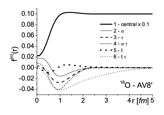
where the term of the order of contains up to the th (dn) power. In Ref. [31], the ground state properties of closed shell nuclei, , and , have been calculated by minimizing the ground state energy at nd order in with respect to the single particle wave functions and the correlation functions . The results for the latter, corresponding to the interaction [32], are shown in Fig. 1.3 versus the distance , in case of . It should be pointed out that:
- •
at relative distances significantly smaller than the average internucleon distance (), nucleons feel the strong central repulsion and the tensor attraction;
- •
at large distances, the effects due to noncentral correlations vanish, the central component is equal to , and the mean field wave function in Eq. (1.17) is recovered.

The net effect generated by the correlation function is demonstrated in Fig. 1.4, where the calculated two-body density distribution for - and - pairs in resulting from the solution of Eq. (1.15) with interaction (1.7), containing the Argonne two-nucleon [34] and Urbana three-nucleon potential [35], is compared with the shell model density solution of Eq. (1.6). It can be seen that, as a result of the contrasting short range central repulsion and the intermediate range tensor attraction, the realistic two-body density strongly differs from the shell model density in the region ; since the average internucleon distance is , we will call the deviation from the shell model in the range short range correlations (SRC), always remembering that they are due to both short range central repulsion and intermediate range tensor attraction, with the latter acting only in and states, and thus enhancing the - distributions. In what follows, it will be shown that SRC strongly depopulate the states below the Fermi sea, creating highly excited virtual two-particle ()- two-hole () states.
1.2 Experimental investigation of long and short range correlations in nuclei

A simple cartoon of NN SRC, as predicted by theoretical calculations, is depicted in Fig. 1.5, and the question arises as to whether such a picture can be experimentally observed. The answer is a positive one, and will be given qualitatively in what follows.
1.2.1 Exclusive lepton scattering: the reaction
A way to learn about correlations in nuclei is represented by the nuclear reaction in which an energetic electron , with energy , knocks out from a nucleus a proton , which is detected in coincidence with the scattered electron , with energy . In this process, the nucleus is left in some excited states with energy , where is the energy transfer (the energy lost by the electron in the scattering process) and and are the kinetic energies of the proton and the residual nucleus, respectively. This kind of nuclear ionization experiments, initiated more than years ago [36], depends upon the number of protons in various shell model states (see 2.3) or, in other words, on the occupation probability in various shell model states, which, as we know, in the single particle shell model is one, for states below the Fermi sea (e.g. and in ), and zero for states above the Fermi sea.
The situation for the nucleus is illustrated in Fig. 1.6.


It can be seen that the first experiments, performed at low energy resolution, identified only two shell model states in , namely and , whereas the high energy resolution experiments [37] demonstrated the occupation [36] of both and shells, as a result of long range correlations (configuration mixing [39]). The occupation numbers of the valence protons in various nuclei obtained from reactions are summarized in Fig. 1.7.

It can be seen that the occupation probability of the least bound (’valence’) nucleons is about ; it strongly deviates from one, i.e. from the prediction of the independent particle shell model. Such a large deviation cannot however be explained only by long range correlations which, as depicted in Fig. 1.6, involve excitation energies of tenth of MeV. It has been argued that the deviation is evidence of SRC which, by populating highly excited states, strongly deplete shell model states below the Fermi sea.
It should be pointed out that, for decades, understanding the role played by SRC in nuclei has been a very elusive problem of nuclear physics, due to the difficulties in isolating the signal of SRC. As a matter of fact, at low and medium energies, effects due to the final state interaction of the knocked out nucleon with the residual system, as well as effects from the excitation energy of hit nucleon, could produce the same final state as the one which is expected to be produced by an initially correlated pair. Investigating SRC thus requires high energy probes, in order to cover kinematical regions with
| (1.29) |
which are available in modern lepton and hadronic accelerators like, e.g., JLab (USA), GSI (Germany) and JPARC (Japan). In Eq. (1.29), is the four-momentum squared of the virtual photon, is the energy transfer, is the nucleon mass, and is the Bjorken scaling variable.
It is only recently that such experiments could be performed, and the excitation strength due to SRC could be observed (cf. Fig. 1.6).
1.2.2 Exclusive lepton scattering: the reaction
Experimentally, high momentum probes can knock out a proton off a nucleus, leaving the rest of the system nearly unaffected. If, on the other hand, the proton being struck is part of a correlated pair, the high relative momentum in the pair leads the correlated nucleon to recoil and be ejected and detected, as pictorially shown in Fig. 1.8. This triple coincidence experiments have been performed on targets, both at Brookhaven National Laboratory (BNL) using incident protons [41, 42, 43], and at Jefferson Laboratory (JLab) by using electrons [5].
The BNL experiment EVA (E850) studied the process


| (1.30) |
with proton beam momentum p ranging from up to .
In the final state, the scattered proton, with momentum , and the knocked out proton, with momentum
| (1.31) |
where q is the momentum transfer, are detected. By assuming that the knocked out proton leaves the nucleus without interacting with the residual system , one has
| (1.32) |
By introducing the so-called missing momentum
| (1.33) |
one has
| (1.34) |
as shown in Fig. 1.9.
If the knocked out nucleon was initially correlated with a neutron, with the nucleus almost at rest, one should observe and detect the recoiling neutron with momentum
| (1.35) |
Within these assumptions, by plotting the momentum of the recoiling neutron as a function of the cosine of the angle between and , i.e.
| (1.36) |
which is known as the number of directional correlations, one should observe, at high values of the momentum , a strong back-to-back directional correlation between and , due to SRC, which has indeed been observed, as shown in Fig. 1.10.

In Ref. [42, 43, 44], the ratio
| (1.37) |
has bee extracted from these data. Eq. (1.37) represents the measure of correlation of backward neutrons with initial momentum , when ; by determining the ratio (1.37) it has been demonstrated that of protons in with momenta are partners in - SRC pairs.

The Jefferson Lab experiment has demonstrated that nearly all nucleons in with momentum in the range - have a correlated nucleon partner with roughly equal and opposite momentum [5, 38]. By comparing - to - pairs yields, it has also been found that SRC are mainly due to - pairs, whose probability results of the order of , as shown in Fig. 1.11 [5]. Calculations explain the magnitude of this - to - ratio as arising from the short range tensor part. Both experiments have shown that recoiling nucleons, with a momentum above the Fermi sea level in the nucleus, are part of a correlated pair, and both observed the same strength of - correlations. This confirms that the process is accessing a universal property of nuclei, unrelated to the probe [45].
1.2.3 Inclusive lepton scattering: the reaction
The high energy reaction depicted in Fig. 1.12, i.e. the process in which only the scattered electron is detected, represents the simplest reaction to investigate SRC and, in particular, to measure the probabilities of SRC in nuclei.

In Ref. [6, 7] it has been supposed that, at high momentum transfer, the inclusive cross section off a nucleus can be written as follows
| (1.38) |
where is the electron-nucleus cross section, written in terms of the -momentum transfer and the Bjorken scaling variable , is the inclusive cross section off a correlated cluster of -particles, and, eventually, the quantity is the probability of finding a nucleon in the cluster . By this way, one expects that the inclusive cross section is dominated, at , by the absorption of the virtual photon on a pair of correlated nucleons and by the elastic rescattering in the continuum, whereas, at , it is governed by three-nucleon correlations (3NC), and so on.
In the process under analysis, as shown in Fig. 1.12, an electron beam with momentum k, knocks out from the nucleus , a nucleon with final four-momentum given by the following energy and momentum conservation
| (1.39) |
where is the four-momentum transfer, and are the momenta of the target nucleus and the residual system , respectively, and is the nucleon mass;

as already pointed out, after interaction only the scattered electron, with momentum , is detected. In Fig. 1.13, the minimum value of the missing momentum
| (1.40) |
defined in terms of the the three-momentum transfer and the momentum of the residual system , is plotted versus the Bjorken scaling variable .
It can be clearly seen that, for any nucleus and fixed , the minimum recoil momentum increases with , and exceeds the average Fermi momentum in nucleus at , the latter depending upon the nucleus [46]. As already pointed out, SRC correspond to high momentum components of the nuclear wave function, therefore, with the gradual increase of , the virtual photon should first probe high momentum configurations due to 2NC and then, following Eq. (1.38), at , it should probe 3NC [6, 7].
To avoid the difficulties due to the theoretical calculations of electron off-shell nucleon cross section, inclusive data from JLab-HallB have been analyzed [4, 46] not directly in terms of cross sections, but by taking the cross section ratios of , and to .

The experimental cross section ratio of nucleus to the nucleus
| (1.41) |
plotted versus the Bjorken scaling variable , is shown in Fig. 1.14. In Eq. (1.41), and are the and inclusive cross sections, respectively, and and are the elementary elastic electron-proton and electron-neutron scattering cross sections. Three different kinematical regions are clearly seen:
- •
: here the shape of the ratio is governed by the different behavior of the magnitude of the quasi elastic peak in different nuclei (higher peaks for light nuclei, and lower peaks for heavy nuclei);
- •
: this plateaux is interpreted as evidence of two-nucleon correlations (2NC), which in complex nuclei and in should differ only by a scale factor;
- •
: the presence of a second plateaux is interpreted as evidence of 3NC.
The relative per-nucleon probabilities and of finding, respectively, 2NC and 3NC in nuclei relative to , extracted from the experimental results shown in Fig. 1.14, are listed in Table 1.1. Here also shown are the absolute (per-nucleon) values and of the same probabilities in nucleus , calculated in Ref. [4] from
| (1.42) | |||
| (1.43) |
by using realistic wave functions of and Deuteron nuclei.
It should be pointed out that no direct calculations of the inclusive cross section ratio shown in Fig. 1.14 have been performed so far. These calculations would represent a relevant contribution towards the solution of the longstanding problem concerning the role played by SRC in nuclei.
In this Thesis, preliminary results of the calculation of the inclusive ratio will be given in Chapter 5, and a new approach [47] to inclusive electron scattering at high momentum transfer will be illustrated.
1.3 Relevance of short range correlations in various fields
As shown in Fig. 1.5, SRC can lead, in small portion of time, to local densities in nuclei comparable with those in the core of neutron stars, i.e. up to times the average nuclear density .

Moreover, combining the results of the various experiments we have illustrated, the probability of finding nucleons in which move in an average potential has been found to be of the order of , whose - due to shell model potential, whereas - due to long range correlations; the remaining represents the SRC contributions, which are dominated by - correlations, due to the strong tensor force which acts between a - pair and does not act in - and - pairs, as shown in Fig. 1.15 [5].
Obtaining information on SRC phenomena in nuclei would have a strong impact on various fields of physics, e.g. in particle-, nuclear- and astro-physics. Let us briefly illustrate some of them:
- -
NN interaction: NN interaction processes at large and intermediate distances are well described in terms of meson exchange, as shown in Fig. 1.16, but such a picture does not allow a proper description of the strongly repulsive NN interaction at short distances. Therefore understanding SRC in nuclei should allow a deeper knowledge of the NN force [48].

Figure 1.16: Hierarchy of scales governing the NN interaction. The distance is given in units of the pion Compton wavelength . After Ref. [48]. - -
Cold dense nuclear matter: the density between correlated nucleons is similar to the one in cold dense nuclear objects, as neutron stars, thus a deep understanding of SRC effects should lead to the formulation of a realistic equation of state for such systems. As shown in Fig. 1.17, the core of neutron stars, neglecting SRC, could be well approximated by two independent Fermi gases: the prevalent one constituted by neutrons, and the smallest one by protons. Even if the number of protons is small, the strong - correlation acts towards the coupling of the two Fermi liquids, thus affecting the equation of state. Moreover, it becomes worth analyzing the role played by SRC phenomena in the URCA processes
(1.44) (1.45) which involve neutrino and antineutrino emission, leading to changes in the physical properties of the system [2].

Figure 1.17: Illustration in momentum space of the momentum distribution, , of protons and neutrons in neutron stars. The left side shows the case where the protons and neutrons weakly interact and can be approximated as separate Fermi spheres, with the neutron momentum much greater than the proton momentum. The figure on the right shows how strong neutron proton SRC cause protons to escape their Fermi sphere and have higher momentum then would otherwise be allowed. After Ref. [45]. - -
Hadron properties: another important problem in modern nuclear physics is given by the modifications of hadron properties such as masses and radii in the nuclear medium. The nuclear EMC effect, i.e. the change in the inclusive deep inelastic structure function of a nucleus relative to that of a free nucleon, induces such modifications, which are of fundamental importance in understanding implications of quantum chromodynamics (QCD) for nuclear physics. As recently shown, possible modifications of nucleon properties induced by the medium can be better studied by analyzing the short range properties of nuclei [49].
- -
QCD: another open problem in modern nuclear and particle physics which could be answered by investigating SRC, concerns the role played by quark and gluon degrees of freedom in nuclear matter at

Figure 1.18: Distances between correlated nucleons are so close that non nucleonic degrees of freedom should reveal themselves. distances, as depicted in Fig. 1.18, which are expected to be most relevant in this interaction range.
- -
High energy scattering processes: recently it has been shown [50, 51] that high energy diffraction effects in nuclei are strongly affected by SRC, which appear to be of the same order as Gribov inelastic shadowing [52]. An example is given in Fig. 1.19 by the total neutron-Nucleus cross section.

Figure 1.19: The neutron-nucleus total cross section, for , , and . Left panel: the result without the inclusion of correlations; dotted curves: shell model contribution; dot-dashed curves: shell model contribution plus inelastic shadowing effects. Right panel: results with the inclusion of correlation. Dotted curves: shell model contribution; dashed curves: shell model contribution plus two-nucleon correlations; solid curves: shell model contribution plus two-nucleon correlations plus inelastic shadowing effects. Experimental data from [53, 54]. After Ref. [50].
A deep comprehension of SRC phenomena is mainly addressed to answer the following questions:
- •
What is the percentage of finding correlated nucleons in nuclei?
- •
What is the relevance of three nucleon SRC in nuclei?
- •
What is the ratio of pp to nn pairs?
- •
Are tensor forces relevant for SRC?
- •
Are these nucleons different from free nucleons?
- •
Which type of analysis should be used in order to obtain information on SRC?
The increasing interest of the scientific community towards the comprehension of SRC in nuclei can be stressed by the large number of conferences and workshops organized in the last year. Some examples are shown in Figs. 1.20-1.23.


Chapter 2 The spectral function and the nucleon momentum distributions: two- and three-nucleon correlations
Introduction
In order to introduce our new approach to the inclusive cross section, it is necessary to recall some basic concepts and general properties about the spectral function and the nucleon momentum distributions.
2.1 The spectral function
The one-body spectral function, which is defined as follows (see e.g. [59])
| (2.1) |
represents the joint probability distribution of finding in the target nucleus a nucleon with momentum and removal energy
| (2.2) |
Here, and are creation and annihilation operators of a nucleon with momentum and spin , respectively; is the intrinsic Hamiltonian of interacting nucleons; is the ground state eigenfunction with eigenvalue , total angular momentum and projection ; eventually, is the mass of the nucleon, the mass of the target nucleus, and the mass of the system , with excitation energy . In what follows, for ease of presentation, the absolute value of a vector a will be indicated as .
By placing in Eq. (2.1) the completeness relation
| (2.3) |
the spectral function becomes
| (2.4) | |||||
where is the intrinsic eigenfunction of the final state of the Hamiltonian with eigenvalue
| (2.5) |
and is the overlap integral
| (2.6) |
where is the two-component Pauli spinor of the nucleon.
Since the set of states also includes the continuum states of the residual -nucleon system, the sum over in Eq. (2.4) stands for summation over the discrete states of the system and integration over the continuum states. Thus the spectral function exactly includes all final states interactions in the states of the system, the only plane wave being that describing the relative motion of the knocked out nucleon and the system.
The spectral function obeys the normalization condition
| (2.7) |
and, owing to Eq. (2.1), it can be written as follows
| (2.8) |
where the contributions from different final nuclear states have been explicitly separated out, namely
| (2.9) | |||||
includes the ground and one-hole states of the ()-nucleon system, and
| (2.10) | |||||
more complex highly excited configurations generated in the target ground state by NN correlations. Here () means that all final states of the residual system below (above) the continuum threshold are considered.
2.2 The nucleon momentum distribution
By definition, the calculation of the spectral function requires the knowledge of the whole set of final states . The calculation of the nucleon momentum distribution requires, on the contrary, only the knowledge of the ground state wave function. As a matter of fact, the momentum distribution is defined as follows
| (2.11) |
where
| (2.12) |
is the non diagonal one-body density matrix.
The spectral function and the momentum distributions are related by the momentum sum rule
| (2.13) |
which is readily obtained by inserting the completeness relation (2.3) in Eq. (2.12).
Within the decomposition rule given by Eq. (2.8), one has
| (2.14) |
with
| (2.15) |
and
| (2.16) |
The integral of the nucleon momentum distributions yields the spectroscopic factors (or occupation probabilities)
| (2.17) |
and
| (2.18) |
which, owing to the normalization condition
| (2.19) |
satisfy the relation
| (2.20) |
Note that, in the independent particle shell model description, as will be discussed in more detail in 2.3, the spectral function can be written as follows
| (2.21) |
where
| (2.22) |
and is the number of nucleons in the state () with removal energy and nucleon momentum distribution .

In Fig. 2.1, the correlated nucleon momentum distributions resulting from the cluster expansion techniques discussed in §1.1 [31] are compared with the mean field component and the variational Monte Carlo calculations [33], in case of . It can be clearly seen that the mean field distributions almost totally exhaust the low momentum part of , and drop to zero at ; on the contrary, because of NN correlations, the high momentum tails are entirely governed by tensor forces, acting in and states which, at high momenta, are several orders of magnitude larger than the predictions from shell model calculations.


Moreover, as shown in Fig. 2.2 and, more clearly, in Fig. 2.3, apart from a scaling factor, the nucleon momentum distributions seem to be almost independent of the atomic weight ; thus, a simple model for the nucleon momentum distributions could be written as follows [60]
| (2.23) | |||||
| (2.24) |
where, because of the effects of correlations, which depopulate states below the Fermi sea, one has
| (2.25) |
and
| (2.26) |
Here the low momentum component, owing to (2.13), is nothing but Eq. (2.21) integrated over the removal energy , with the shell model momentum distribution replaced by the modified ones which takes into account the effects of correlations; on the contrary, the high momentum part is nothing but the Deuteron nucleon momentum distribution rescaled by a constant , which depends on the nucleus under consideration, and whose values are listed in Table 2.1. We call such a behavior Deuteron scaling.
Deuteron scaling is even more pronounced in the the two-nucleon momentum distributions, defined as follows
| (2.27) |
which have recently been calculated in Refs. [9, 31].
The knowledge of allows one to calculate the relative and center of mass (CM) momentum distributions of a two-nucleon pair , i.e.
| (2.28) | |||
| (2.29) |
where
| (2.30) |
are the relative and CM momenta of the pair -, respectively, with and being measured from the CM of the system, and
| (2.31) |
is the off-diagonal two-body density matrix.
Deuteron scaling can be clearly seen in Figs. 2.4, 2.5 and 2.6, where


the quantity , describing back-to-back nucleons, is plotted versus the relative momentum . These figures clearly illustrate the dominant role of the tensor forces in producing a substantial difference between - and - two-nucleon momentum distributions, both in few-nucleon systems and complex nuclei.
In Ref. [10], the following ratio
| (2.32) |
which represents the percentage probability of finding a - pair in the nucleus , has been calculated. The results, listed in Table 2.2, show that is proportional to the percentage of - pairs, when integration runs over the whole range of ; on the contrary,
when integration is limited to the correlation region, the percentage of - pairs results much larger than that of - pairs, which is a clear consequence of the effects of the tensor forces acting between a proton and a neutron.
2.2.1 The saturation of the momentum sum rule

A relevant relationship between high momentum and high removal energy components can be obtained by considering the partial momentum distribution [62]
| (2.33) |
where the upper limit of integration can be varied from to . By definition, Eq. (2.33) represents that part of which is due to final -nucleon states with . In the limit one gets
| (2.34) |
and the momentum sum rule given by Eq. (2.13) is recovered. Thus the behavior of as a function of provides information on the saturation of the momentum sum rule and the relevance of binding effects.
The saturation of the momentum sum rule for [62] and Nuclear Matter [65] is shown in Fig. 2.7, using realistic spectral functions. It can be clearly seen that, at , the momentum sum rule is saturated already at values of very close to , whereas at , on the contrary, the momentum sum rule is saturated only when high values of are considered. This can be explained in terms of the spectral function appearing in Eq. (2.33) which, at low momenta, is dominated by its component , whose strength is almost totally concentrated at low values of the removal energy; at high momenta, on the contrary, it depends upon , spread, for a given , over a wide range of values of .
2.2.2 Probabilities of independent particle and correlated momentum components
Let us define
| (2.35) |
and
| (2.36) |
as the probability of finding independent particle and correlated momentum components in nucleon momentum distributions, with ranging from to . When , the spectroscopic factors given by Eqs. (2.17) and (2.18) are recovered.
The values of these two quantities, calculated for different values of and for different nuclei, are listed in Table 2.3.
| [fm-1] | ||||||
It can be seen that:
- •
when the whole range of the momentum is considered, the probability of finding independent particle low momentum shell model components is much larger than the probability to find correlated high momentum components;
- •
for the contribution from shell model and correlated nucleons is comparable;
- •
for the probability of finding shell model nucleons is still different from zero, but orders of magnitude less than the probability due to correlated nucleons.
Let us now discuss in more detail the low and high momentum components of the nuclear wave function.
2.3 Low momentum components and the mean field structure of the nuclear wave function
Eq. (2.9) yields the probability distribution that the final -nucleon system is left into its ground state, i.e. with and . As already pointed out, the shell model spectral function can be written as follows
| (2.37) |
with denoting the number of nucleons in the state with removal energy and nucleon momentum distribution . At the same time, one has
| (2.38) |
In Eq. (2.37), the sum over runs only over the hole states of the target, which means that the occupation probability is
The main effect of NN SRC is to deplete states below the Fermi level and to make the states above the Fermi level partially occupied. By such a mechanism
| (2.42) |
and
| (2.43) |
Disregarding the finite width of the states below the Fermi level, the modified shell model contribution can be written as
| (2.44) |
where the occupation probability for hole states is
| (2.45) |
Eq. (2.44) drops down very quickly for and , where the spectral function behavior is governed by NN correlations, and thus by its correlated component .
2.4 Two-nucleon correlations


In Fig. 2.8(a) the spectral function of corresponding to the AV18 interaction [20] is shown versus the momentum and the removal energy . A typical feature of the spectral function, common also to the spectral function of Nuclear Matter [63, 64], is that it exhibits, at high values of and , broad peaks located at
| (2.46) |
and whose width increases with , as clearly exhibited in Fig. 2.8(b), where some cuts of are shown. Eq. (2.46) is generated by 2NC in nuclei, as will be demonstrated in what follows, by illustrating different model developed in the last few years, differing in the description of the nucleon configurations inside the nucleus.

To this end, in Fig. 2.9, a simple cartoon of a target nucleus and its nucleon constituents is given.
2.4.1 The naive two-nucleon correlation model

In Ref. [6, 7], a first microscopic model leading to Eq. (2.46) has been proposed. It is based upon the assumption that, referring to Fig. 2.10, the high momentum of nucleon ’’ is entirely balanced by the momentum of nucleon ’’, whereas the residual spectator system has total momentum . Energy conservation for such a mechanism requires that
| (2.47) |
where
| (2.48) |
is the recoil energy of the residual -nucleon system, whose intrinsic excitation energy could therefore be written as
| (2.49) |
Within such a picture, the nucleon spectral function simply reads as follows
| (2.50) |
where
| (2.51) |
is the two-nucleon breakup threshold, being and the (positive) ground state energies of nucleus and .
2.4.2 The convolution formula
The naive 2NC model has been implemented in [60, 68], by assuming that the momentum of nucleon ’’ is not fully balanced by the momentum of nucleon ’’, but also by the residual system, as depicted in Fig. 2.11; in other words, it is assumed that the spectator system moves with small momentum . We will call such a configuration few nucleon correlation (FNC) configuration.

Introducing the previously defined center of mass, , and relative, , momenta of the correlated pair as follows
| (2.52) | |||||
| (2.53) |
momentum conservation yields
| (2.54) | |||
| (2.55) |
and energy conservation reads as follows
| (2.56) |
where
| (2.57) |
is the energy of the relative motion of particles ’’ and ’’, i.e. the excitation energy of the residual system. In Eq. (2.57), eventually,
| (2.58) |
is the reduced mass of particles ’’ and ’’.
Given these assumptions, the spectral function, at high and high , has been obtained in Ref. [60] by assuming that the ground state wave function of nucleus factorizes as follows
| (2.59) |
where
| (2.60) |
are the relative and CM coordinates, respectively, with , is a proper antisymmetrization operator, and is a short-hand notation for the standard Clebsh-Gordan coupling of orbital and spin angular momenta; and represent a complete set of states describing the relative and CM motion of the pair, and, eventually, is the complete set of states describing the -nucleon system.
As already explained, SRC correspond to the high momentum and high removal energy components of the spectral function . In momentum space, SRC are described by a correlated pair with a very high relative momentum , and a low CM momentum ; the latter condition justifies the choice of the CM motion in -state, so that
| (2.61) |
where describes the low momentum CM wave function in -state. Since the -wave motion also implies that the system is in the ground state or in a low energy excited state, one can write, eventually, [60]
| (2.62) |
where
| (2.63) |
describes the relative motion of the correlated pair in the nuclear medium. In Eq. (2.62), denotes the excitation spectrum of the system which, since, as already pointed out, the CM of the pair involves only low momentum components, have been mainly limited to the ground state and to the (low-lying) excited states corresponding to configurations generated by the removal of two particles from different shell model states of the target.
The above formalism leads to the following convolution formula, involving only the relative and CM momentum distributions of the correlated pair
| (2.64) | |||||
where and are the momentum distributions of the relative and center of mass motion of the two nucleons in a correlated pair, respectively, and the other notations, following Fig. 2.9, are self explaining; eventually, the factor satisfies the normalization condition given by Eq. (2.7). We stress once again that in such an approach, the residual -nucleon system is assumed to be in its ground state, which implies that the CM of the correlated pair moves with low momentum, so that only ”soft” components of contribute to the spectral function , since we have seen in Chapter that high momentum components of a nucleon are linked to high excitation energies of () and this has to be true also for the system (-)-().

The naive 2NC model is recovered by placing
| (2.65) |
i.e. by assuming that the spectator nucleus is at rest.
Integrating Eq. (2.64) over and the angular variables of , one gets
| (2.66) |
where
| (2.67) | |||||
| (2.68) | |||||
| (2.69) |
The convolution formula (2.66) has been calculated in Ref. [60] by using the following effective relative and CM nucleon momentum distributions
| (2.70) |
and
| (2.71) |
respectively, with the parameter determined as explained in Ref. [60].

Recently, and have been obtained from many-body approaches [9, 10], separately for - and - pairs, and they quantitatively agree with the forms given by Eqs. (2.70) and (2.71).
In such a way, the convolution formula (2.66) is completely defined in terms of many-body quantities.
Eventually, it should be pointed out that, in the recent BNL experiment on target [38], the CM momentum distribution has been measured, finding that it fully agrees with the prediction of Ref. [60], as shown by the full line in Fig 2.13.
2.5 Brueckner-Bethe-Goldstone theory and the validation of the convolution formula
The convolution model can be microscopically derived from the Bruckner-Bethe-Goldstone (BBG) theory [69]. Let us discuss this aspect in more detail.
In nuclear matter the spectral function corresponding to the nucleon self-energy
| (2.72) |
is given by the well known result [59]
| (2.73) |
where is the single-particle Green function
| (2.74) |
It has be noticed that the real, , and imaginary parts, , of the self-energy are highly off-shell in the considered energy and momentum ranges. We are interested in the region where is much greater than the Fermi energy ; for high and , one has
| (2.75) |
and Eq. (2.73) becomes
| (2.76) |
where denotes a ”particle state” (outside the Fermi sea), and a ”hole state” (inside the Fermi sea), with energies , and respectively, and is the BBG scattering matrix
| (2.77) | |||||
where is the Pauli projection operator, which restricts the two nucleons in intermediate states to lie outside the Fermi sea. It should be stressed that Eq. (2.76) corresponds to the - diagram of Fig. 2.14 which, through the G matrix, sums up all ”ladder diagrams” where the BBG scattering matrix is replaced by the bare NN interaction.

Eq. (2.76) can be expressed in terms of the defect wave function, defined as
| (2.78) |
where is the correlated two-body wave function, and the uncorrelated one. After a length algebra, one finds [69]
| (2.79) |
where
| (2.80) |
is the nuclear matter density and
| (2.81) |

2.6 Many-body validation of the factorization of the nuclear wave function at high momenta
In this section, we will show that the convolution formula results from a rather general property of the nuclear wave function. Let us recall that the convolution formula has been obtained by assuming that the nuclear wave function factorizes into the wave function of a correlated pair and the wave function of a core of the -nucleon system. In Ref. [70], the s-wave three-body Faddeev wave function obtained with [71] potential has been used to calculate the following quantity
| (2.82) |

where
| (2.83) |
is the two-nucleon relative coordinate,
| (2.84) |
the CM coordinate, and the angle between them. If the ratio (2.82) is plotted versus for fixed values of , and , exhibits a constant behavior; this is evidence of the factorization of in the variable and . As a matter of fact, it can be seen that writing
| (2.85) |
one gets
| (2.86) |
The results presented in the upper panel of Fig. 2.16 clearly show that, when is large and small, indeed factorizes. On the contrary, as shown in the lower panel of Fig. 2.16, for small values of and small values of , the nuclear wave function does not factorize. Thus the factorization of the nuclear wave function at high momenta is validated by many-body wave functions.
2.7 Three-nucleon correlations
2.7.1 Naive three nucleon correlation models
We have seen that the high momentum and high removal energy components of the nuclear spectral function are due to few nucleon correlations (FNC), in particular in the region around
| (2.87) |

FNC cannot however explain the regions at high values of and large values of the excitation energy
| (2.88) |
and the region at high values of and low values of
| (2.89) |
This can be clearly seen in Fig. 2.17. In these regions, one has to consider the effects of three-nucleon correlations (3NC), i.e. configurations characterized by three nucleons which have comparable momenta, and share almost the full momentum of the nucleus
| (2.90) |
i.e.
| (2.91) |

The naive 3NC model will be defined as follows: referring to Fig. 2.18, we will consider that the high momentum of nucleon ’’ is completely balanced by the high momenta and of particle ’’ and ’’, respectively, with the residual -nucleon system at rest.
Within such a naive model, the residual system has momentum
| (2.92) |
and excitation energy
| (2.93) |
given by the relative motion of particle ’’ and the residual -nucleon system, with reduced mass
| (2.94) |
The excitation energy of the residual system can be written as follows
| (2.95) |
i.e. by considering both the contribution arising from 2NC, given by Eq. (2.57), and the one due to 3NC, given by Eq. (2.93). It can be clearly seen from Fig. 2.18, and it will be explained in more detail in 4.3, that the assumptions of the naive model for three correlated nucleons refer only to that values of given by Eq. (2.89).
The 3NC contribution to the spectral function , given by Eq. (2.10), turns out to be [72]
| (2.96) |
where is necessary to satisfy the normalization condition (2.7). It should be pointed out that Eq. (2.96) is nothing but Eq. (2.64) with replaced by .

A first approximation to Eq. (2.96) could be obtained by considering
| (2.97) |
with
| (2.98) |
and
| (2.99) |
as shown in Fig. 2.19.
In this case, the ”hard” CM nucleon momentum distribution will read as follows
| (2.100) |
and the removal energy will reduce to
| (2.101) |
Integrating Eq. (2.96) over the momentum , yields
| (2.102) |
Chapter 3 Inclusive electron scattering off nuclei at high momentum transfer and final state interaction effects: results of calculations
Introduction
Inclusive electron scattering off nuclei at high momentum transfer can provide non trivial information on nuclear wave function. In particular, the kinematic region corresponding to is

strongly affected by high momentum and high removal energy components of the nuclear wave function arising from NN SRC.


The Feynman diagram depicted in Fig. 3.1 describes the inclusive cross section which, as is well known, in one photon exchange has the following form
| (3.1) |
where
| (3.2) |
is the Mott cross section, which describes the scattering from a pointlike nucleon,
| (3.3) |
is the squared four-momentum transfer, is the scattering angle and are the nuclear structure functions.
In plane wave impulse approximation (PWIA), shown in Figs.3.2(a) and 3.2(b), the latter are given by
| (3.4) |
where , are the nucleon structure functions, and are kinematical factors whose explicit expression is given e.g. in [74], and, finally,
| (3.5) |
where is the four-momentum of the struck off-shell nucleon.
According to the value of the invariant mass produced by the interaction of the virtual photon with a nucleon in the nucleus, the inclusive process is governed by the following two mechanisms: i) the quasi elastic (qe) process, for which , and ii) the deep inelastic scattering (DIS), corresponding to . The basic nuclear quantity that governs qe and DIS processes at is the nucleon spectral function.
The PWIA is only the first approximation to the calculation of the cross section, since the final state interaction (FSI) of the struck nucleon with the residual system () may play an important role. As increases, the effects due to the FSI in the qe process are expected to decrease, whereas the DIS contribution increases.
In this Thesis, we will focus only on the qe process. Two types of FSI in the qe process, to be considered in what follows, are shown in Fig. 3.2(c) and 3.2(d).
3.1 The quasi elastic cross section
In PWIA, the qe inclusive cross section describing the knock-out by the incoming electron of a nucleon from the nucleus , can be written as follows [12]
| (3.6) |
The argument of the energy conserving -function is
| (3.7) |
where
| (3.8) |
is the mass of the excited residual system, and momentum conservation reads as follows
| (3.9) |
Here and are the energy and three-momentum transfers, is the elastic electron cross section off a moving off-shell nucleon with momentum and removal energy , and are the momenta of the undetected struck nucleon and the final system; eventually, is the nucleon spectral function discussed in the prevous chapter. From now on, for ease of presentation, only isoscalar nuclei, i.e. with , will be considered.
After integrating over , Eq. (3.6) becomes
| (3.10) | |||||
where the limits of integration [75]
| (3.11) | |||||
| (3.12) | |||||
are imposed by energy conservation, where
| (3.15) |
is the invariant mass,
| (3.16) |
and the phase space factor
| (3.17) |
results from the dependence upon of the nucleon energy in the final state in the -function. Eventually,
| (3.18) |
is the electron-nucleon cross section for a relativistically moving nucleon, averaged over the polar angle, where , , , and .
At high momentum transfer, the quantity
| (3.19) |
depends very weakly upon , so that it can be taken out of the integral and evaluated, e.g., at . Therefore Eq. (3.10) can be written in the factorized form
| (3.20) |
where
| (3.21) |
is the nuclear structure function.
3.2 The scaling function
At high values of the momentum transfer, the rapid falloff of with and allows the replacement , and Eq. (3.21) can be written as
| (3.22) |
Therefore, the structure function depends upon and only through , which is determined from the energy conservation (3.7).
Let us replace the energy transfer with a generic scaling variable
| (3.23) |
which is only required to be a function of and (and any arbitrary constant) so that, no matter with the specific form of , the cross section and the structure function can be expressed not in terms of the two canonical independent variables and , but, without loss of generality, in terms of and . Correspondingly, a scaling function is introduced, which is nothing but Eq. (3.22) with replaced everywhere by ; if, under certain conditions, reproduces the asymptotic scaling function
| (3.24) |
Y-scaling is said to occur and, depending on the physical meaning of and , various information on nucleons in nuclei could be obtained.
Using Eq. (2.8), the scaling function becomes
and it can be trivially cast in the form
| (3.26) |
where the longitudinal momentum distribution
| (3.27) |
is integrated over all excited states of , whereas the binding correction
| (3.28) |
on the contrary, is governed through by the continuum energy spectrum of the final system. The contribution arising from the latter strongly depends by the difference between and and, therefore, upon the definition of the former. In the Deuteron case, in fact
| (3.29) |
| (3.30) |
and thus
| (3.31) |
| (3.32) |
Therefore, when the binding correction can be neglected, as in the Deuteron, the quantities and are linked by the relation
| (3.33) |
so that, if could be extracted from the experimental data, could be
determined.
Unfortunately, in general, such an extraction is hindered by the presence of
| (3.34) |
which leads to
| (3.35) |
and
| (3.36) |
The factorization given in Eq. (3.26), in the asymptotic limit reads as
| (3.37) |
but again, unfortunately, owing to the presence of , is not related to a momentum distribution, so that, in principle, the experimental longitudinal momentum distribution and, consequently, , cannot be extracted from the data.
In both Eqs. (3.24) and (3.26), the contribution arising from the binding correction depends upon the difference between and , which could be minimized only by a proper choice of the scaling variable , such that . The resulting cross section (3.6) would depend only upon the nucleon momentum distributions, obtaining, by this way, a direct access to high momentum components generated by SRC [76]. It is clear that the outlined picture can in principle be modified by the effects of the FSI of the knocked nucleon with the residual -nucleon system.
3.3 The final state interaction
Owing to the decomposition rule (2.8) of the spectral function , the inclusive cross section can be written in the following form
| (3.38) |
where describes the transition to the ground and one-hole states of the -nucleon system, and the transition to more complex highly excited configurations.
The diagrams in Figs. 3.2(a) and 3.2(b) refer, respectively, to the contribution of and in PWIA, which is based upon the assumption that the reaction is well described by the exchange of a single virtual photon with a single nucleon, which does not interact with the remaining -nucleons; in particular, the diagram 3.2(a) represents the contribution arising from shell model configurations, whereas the diagram 3.2(b) mainly describes absorption by - configurations generated in the target ground state by NN correlations. It is well known that the PWIA sizably underestimates the cross section, both in light and heavy nuclei, at low values of , i.e. at , owing to FSI processes which arise from the interaction between the knocked out nucleon and the residual system.
In this Thesis, following the approach proposed in Ref. [73], we take into account two different FSI processes, i.e.: i) the two-nucleon rescattering in the final state when the struck nucleon is a partner of a correlated pair, shown in Fig. 3.2(d), and ii) the single-nucleon rescattering of the struck nucleon with the mean optical potential of the residual system, depicted in Fig. 3.2(c). Let us discuss in more detail these two mechanisms.
3.3.1 Two-nucleon rescattering
The basic assumption underlying the convolution formula (2.66), is that two nucleons are locally strongly correlated at short separations, with their CM being apart from the spectator -nucleon system. 2NC in a nucleus are reminiscent of correlations in the Deuteron; indeed, as discussed in 2.2, nucleon momentum distributions of light and complex nuclei, at , turn out to be the properly rescaled version of the Deuteron momentum distribution.


Therefore, in the 2NC region, the absorption of by a correlated pair is expected to resemble the one in the Deuteron; if so, such a Deuteron-like picture of the initial state should be extended also to the final state by allowing the two nucleons to elastically rescatter, as depicted in Fig. 3.2(d).
An important difference from the Deuteron case is that a correlated pair in a nucleus is bound and moves in the field created by the other nucleons.
Within the above picture, the contribution of diagrams 3.2(a)-3.2(d) reads as follows [73]
| (3.39) | |||||
| (3.40) |
where
| (3.41) | |||||
| (3.42) |
represents the (reduced) leptonic tensor, and is the hadronic tensor of a correlated pair, which can be written as follows
| (3.43) | |||||
where is the nucleon current, , is the relative wave function of the initial state of a correlated pair, and its continuum final state. Eq. (3.40) is based upon the following assumptions on final and initial -nucleon state:
| (3.44) | |||||
| (3.45) |
where is a proper antisymmetrization operator, is the CM wave function of the initial state of a correlated pair, and its plane wave final state. It can be seen from Eq. (3.43) that medium effects on the hadronic tensor of the pair are generated by the energy conserving -function, in which the intrinsic energy available to the pair is fixed by its CM four-momentum, and, therefore, by the momentum distribution appearing in Eq. (3.40). Even if the CM motion is neglected by placing
| (3.46) |
medium effects still would remain through the quantity
| (3.47) |
which is related to the two-nucleon break up threshold, i.e. the binding of the pair.
The inclusive cross section have been calculated in [73] for the Deuteron using the RSC NN potential [79], taking into account the rescattering in S, P and D partial waves; then, using the same two-nucleon amplitudes , the cross section have been computed for complex nuclei. The results are shown by the dashed lines in Fig. 3.3: it can be seen that, at , the process of two-nucleon rescattering brings theoretical predictions in good agreement with experimental data. The most striking aspect of these results is that the same mechanism which explains the Deuteron data, does the same in a complex nucleus, provided the A dependence due to and (clearly exhibited in Fig. 3.3) is properly considered. It should be pointed out that these results hold for the whole set of kinematics considered in Refs. [13, 81, 82, 83].
3.3.2 Single nucleon rescattering
The two-nucleon rescattering is not able to describe the experimental data at . This fact is not surprising because, at , more than two nucleons should be involved in the scattering process. This process can be simulated by considering the motion of the nucleon, knocked out from shell model states, in the optical potential generated by the ground state of the -nucleon system. Within such an approach, corresponding to diagrams 3.2(a)-3.2(c), Eq. (3.39) becomes [73]
| (3.48) |
resulting from the eikonal approximation for the nucleon propagator [84]. The optical potential can be cast in the following on-shell form
| (3.49) |
where is the nuclear density, is the nucleon velocity, is the total NN cross section and is the ratio of the real to the imaginary part of the forward NN scattering amplitude. The imaginary component of Eq. (3.49) describes inelastic processes leading to excitations of the residual system, which, in the high energy regime, mainly correspond to secondary nucleon emissions.
It has be pointed out [73], that the two-nucleon rescattering is not included in the process described by diagram 3.2(c). As a matter of fact, indeed, the two-nucleon rescattering is not a multiple scattering process, i.e. it does not contribute to an optical potential, and, particularly, is independent of nuclear density and does not produce any absorption of the outgoing flux.
However, treating FSI at in terms of on-shell potentials is not justified [6, 7, 85, 86]. Indeed, the struck nucleon, with momentum
| (3.50) |
can be either on-mass-shell, i.e. with , or off-mass-shell, namely with , depending on the values of and . Initial configurations with give rise to an intermediate off-mass-shell virtual nucleon, so that the use of an on-shell optical potential is unjustified, and can hardly be reconciled with the fact that rescattering amplitudes are expected to decrease with virtuality, because an off-shell nucleon has to rescatter within short times. Therefore, in order to take into account off-shell effects, we have to include in a suppression factor of the type
| (3.51) |
The differences between the use of an on-shell or off-shell potential are shown in Fig. 3.4. The parameter appearing in Eq. (3.51) is the same for all kinematics considered.

3.4 Inclusive cross sections: results of calculations
The results of our calculations, including the contributions from all diagrams depicted in Fig. 3.2, are shown in Figs. 3.5 and 3.6.


It can be seen that the PWIA overestimates the experimental data at , whereas the inclusion of the FSI produces a good agreement between theoretical calculations and experimental data. In the region , the FSI is mainly due to the two-nucleon rescattering whereas, at , the contribution from the optical potential, which mocks up three-nucleon correlation effects, becomes important. Other results are shown in Figs. 3.7 and 3.8, leading to the same conclusions. Results of the same quality were previously obtained in Ref. [17, 18, 73].


Chapter 4 A novel approach to scaling phenomena in inclusive scattering: mean field, correlations and proper scaling variables.
Introduction
The inclusive cross section can be analyzed in terms of scaling function and scaling variable.
The scaling variable arises from the energy conservation law which, for an inclusive process, reads as follows
| (4.1) |
being
| mass of the target nucleus | (4.2) | ||||
| mass of the residual nucleus | (4.3) | ||||
| intrinsic excitation energy of the residual system | (4.4) | ||||
| mass of the knocked out nucleon | (4.5) |
As mentioned in Chapter 2, a proper choice of the scaling variable could minimize the contribution arising from the binding correction, allowing a direct link between the scaling function and the nucleon momentum distribution. Within such an approach, the new inclusive cross section for electron scattering off nuclei can be written only in terms of nucleon momentum distributions, so that inclusive scattering becomes a powerful tool to investigate NN SRC in nuclei. In what follows, it will be illustrated in detail how the dependence of upon gives rise to the binding correction, and how to a different definition of the scaling variable .
4.1 The mean field scaling variable
The final state interaction of the struck nucleon invalidates the PWIA but, in spite of that, an approach was developed in the past to reduce the effects from both the binding corrections and FSI [11, 75]; the traditional approach to Y-scaling is based upon the traditional scaling variable , obtained by placing
| (4.6) |
| (4.7) |
| (4.8) |
in the energy conservation law given by Eq. (4.1), obtaining
| (4.9) |
whose solution is [12]
| (4.10) |
with
| (4.11) |
and
| (4.12) |
Within such an approach, represents the minimum longitudinal momentum of a nucleon having the minimum value of the removal energy
| (4.13) |
At high values of , one has
| (4.14) |
so that, when ,
| (4.15) | |||||
| (4.16) |
and thus the scaling function reduces to
| (4.17) |
explicitly showing scaling in .

Unfortunately, this occurs only in the Deuteron, whereas in the general case, for , the excitation energy of the residual system is different from zero and
| (4.18) |
leading to
| (4.19) |
and thus to the relation , given by Eq. (3.26).
To illustrate the relevant role played by the binding correction in the traditional approach to Y-scaling, the ratio
| (4.20) |
which represents the deviation of the scaling function from the longitudinal momentum distribution , is shown in Fig. 4.1, plotted versus the scaling variable . It can be seen that, at high values of , the effects from binding are very large whereas, at low values of , binding effects can be neglected.

Moreover, the experimental scaling function
| (4.21) |
plotted versus the scaling variable , as shown in Fig. 4.2, confirms that the scaling function strongly differs from the longitudinal momentum distribution, and therefore does not exhibit any proportionality to the Deuteron scaling function . Therefore it should be pointed out that, when expressed in terms of , a comparison between experimental and theoretical scaling functions requires the knowledge of the nucleon spectral function, generated by the main role played by .
Moreover, the experimental scaling function exhibits a strong dependence owing to the FSI and binding effects, and differs from the asymptotic scaling function . The latter, however, has been obtained in Ref. [11, 75] by extrapolating to the available values of , on the basis that FSI can be represented as a power series in , and dies out at large , a conclusion that has been reached by various authors (see e.g. [89]).
It is therefore the dependence of upon that gives rise to the binding effect. This is an unavoidable defect of the usual approach to Y-scaling, based on
the scaling variable ; except for the trivial case of the Deuteron, in fact, in a complex nucleus the final -nucleon system can be left in all possible excited states, including the continuum but, by definition, the traditional scaling variable can only be identified with the longitudinal momentum of weakly bound, shell nucleons (). The longitudinal momentum for such nucleons is very different from the strongly bound, correlated nucleons (), and this explains why, at large values of , the scaling function is not related to the longitudinal momentum of strongly bound correlated nucleons, whose contributions almost entirely exhaust the behavior of the scaling function.
As stressed in Refs. [16, 17, 18], to establish a global link between experimental data and longitudinal momentum components, one has to conceive a scaling variable that could equally well represent longitudinal momenta of both weakly bound and strongly bound nucleons, so that the binding correction could be minimized.
The experimental longitudinal momentum distribution has thereby been obtained by adding to the binding correction evaluated theoretically, as shown in Fig. 4.3, and has been obtained by Eq. (3.36). Such a procedure affects the final results in terms of large errors on the extracted
momentum distributions, particularly at large values of ; in spite of these errors, the extracted momentum distributions, at , turned out to be larger by orders of magnitude from the prediction of mean field approaches, and in qualitative agreement with realistic many-body calculations that include SRC.
In order to make the extraction of as independent as possible from theoretical binding corrections, in Ref. [16] is thus necessary to introduce another scaling variable, incorporating relevant physical dynamical effects left out in the definition of .

4.2 Two-nucleon correlation scaling variable
2NC are defined, as previously explained in 2.4, as those nucleon configurations shown in Fig. 4.4 [3]: momentum conservation in the ground state of the target nucleus
| (4.22) |
is almost entirely exhausted by two correlated nucleons with high momenta, the -nucleon system acting mainly as a spectator, moving with very low momentum.
The intrinsic excitation energy of the -nucleon system is in this case
| (4.23) |
which becomes
| (4.24) |
in the naive 2NC model, i.e. the model based upon the assumption . Since high excitation states of the final -nucleon system are generated by SRC in the ground state of the target nucleus, the traditional (mean field) scaling variable does not incorporate, by definition, SRC effects, for it is obtained by placing in the energy conservation law (4.1). Motivated by this observation, in Ref. [16], a new scaling variable, has been introduced, by setting
| (4.25) |
| (4.26) |
| (4.27) |
in Eq. (4.1), which in this case reads as follows
| (4.28) |
The inclusion of the term
| (4.29) |
makes the scaling variable to properly depend upon the momentum dependence of the average excitation energy of , generated by two-nucleon correlations. Here
| (4.30) |
where
| (4.31) |
is the threshold energy for two-particle emission.
The quantity in Eq. (4.29) has been calculated using a realistic spectral function for nuclear matter and
. The results are presented in Fig. 4.5, where they are compared with the prediction of the spectral function of the few nucleon correlation (FNC) model of Ref. [60], according to which
| (4.32) |
where is the CM momentum of a correlated pair. In view of the very good agreement between the FNC model and the exact many-body results for nuclear matter and , the former has been used to calculate for nuclei with .
The values shown in Fig. 4.5 can be interpolated by
| (4.33) |
where
| (4.34) |
and
| (4.35) |
| (4.36) |
result from the CM motion of the pair.

The values of and used in our calculations are listed in Table 4.1.
| Nucleus | (MeV) | |
|---|---|---|
For a complex nucleus and not too large values of , a solution for Eq. (4.28) can be written as
| (4.37) |
where
| (4.38) |
| (4.39) |
| (4.40) |
| (4.41) |
In order to counterbalance the effects of at low , in the definition of
| (4.42) |
has been added the value , fixed by the Koltun sum rule (see [16, 17, 18]).
In the Deuteron case
| (4.43) |
with
| (4.44) |
and where
| (4.45) |
is the Deuteron invariant mass.
For small values of , such that
| (4.46) |
the variable , representing the longitudinal momentum of a weakly bound nucleon,
is recovered.
Therefore effectively takes into account the dependence of , both at low and high values of , and interpolates between the correlation and the single-particle regions; it can be interpreted as the minimum longitudinal momentum of a nucleon that, at high values of , has removal energy and is partner of a correlated two-nucleon pair with effective mass .
It should be pointed out that, in our calculations, the fourth-order equation resulting from Eq. (4.28) has been solved exactly; this, together with the relativistic extension of the definition of the mean excitation energy, is necessary to extend to high values.

Within such an approach to Y-scaling, the effects due to the binding are strongly suppressed, as clearly illustrated in Fig. 4.6, where the ratio given by Eq. (4.20) vanishes in the whole region of considered; the main feature of , in fact, is that
| (4.47) |
which leads to
| (4.48) |
with the following two relevant consequences:
- 1.
the relation
(4.49) holds, thus, plotting the data in terms of can provide a direct access to the nucleon momentum distributions, and so to SRC in nuclei;
- 2.
as mentioned in , many-body calculations show that at high momenta, , all nucleon momentum distributions are simply rescaled version of the Deuteron one, i.e.
(4.50) where is a constant; as a consequence, one would expect that, at high values of , will behave in the same way in the Deuteron and in complex nuclei, so that, accordingly,
(4.51) At the same time, on the contrary, at low values of , should exhibit an dependence generated by the different asymptotic behavior of the nuclear wave functions in configuration space.


This is fully confirmed by Fig. 4.7, where the scaling function obtained from available experimental data on , and , is plotted versus the scaling variable ; it can be seen that, at high values of , scales exactly to . This is even better demonstrated in Fig. 4.8, where the scaling function is plotted versus at fixed values of . By this way, the scaling behavior of is better illustrated. In the same Figure, in order to analyze more quantitatively the scaling behavior of , the latter has been plotted together with the theoretical scaling function for , calculated in PWIA (solid line), and taking FSI into account (dashed line). The left panel clearly illustrates that, due to FSI effects, scaling is violated and approached from the top, and not from the bottom, as predicted by the PWIA. However, scaling violation seems to exhibit a dependence which is very similar in Deuteron and in complex nuclei. This is illustrated in more details in the right panel of the Figure, which shows the quantity
| (4.52) |
where the dependent constants have been chosen so as to make the experimental scaling function for a nucleus to coincide as much as possible with the Deuteron scaling function . It clearly appears that the scaling functions of heavy and light nuclei scale to the Deuteron scaling function; moreover the values obtained for turn out to be in agreement, within the statistical errors, with the theoretical predictions of Ref. [6], as well as with the experimental results on the ratio [3]
| (4.53) |

shown in Fig. 4.9; it is also important to stress that, although FSI are very relevant, they appear to be similar in Deuteron and in a nucleus A, which is evidence that, in the SRC region, FSI are mainly restricted to the correlated pair.
4.3 Three-nucleon-correlation scaling variable
Three-nucleon correlations also contribute, in principle, to the inclusive cross section for . 3NC correspond, as previously explained in 2.7, to those three-nucleon configurations in which the high momentum of nucleon ”1” is almost entirely balanced by the momenta and of nucleons ”2” and ”3”, respectively.
The excitation energy of the -nucleon system is given in this case by (Cf. Eq. (2.95)) [47]
| (4.54) |
which shows that, whereas 2NC are directly linked to high values of excitation energies
| (4.55) |
high momentum components due to 3NC may lead both to low and to high values of , as shown in the examples of Figs. 4.10(a) and 4.10(b), respectively.


In the configuration of Fig. 4.10(a), the momentum of nucleon is almost entirely balanced by nucleons and , with momenta , and one has
| (4.56) |
In the configuration of Fig. 4.10(b),
| (4.57) |
with
| (4.58) |
and could be very large when and are large.
Let us investigate the presence and relevance of 3NC configurations in the spectral function of the 3N system, for which the Schrdinger equation has been solved exactly. When , 3NC of the type shown in Fig. 4.10(a) lead to (cf. Eq. (4.56)).
In Fig. 4.11, as already illustrated in 2.7, the realistic spectral function of obtained [66] using the Pisa wave function [90] corresponding to the AV18 interaction [20] (full squares), is compared with the predictions of the FNC model (solid line) given by the convolution formula (2.66) [47]. It can be seen that the FNC spectral function reproduces the exact one in a wide range of removal energies (), but fails at very low and very high values of E, where the effects from 3NC are expected to provide an appreciable contribution.
It is clear from Fig. 4.11 that 3NC of the type shown in Fig. 4.10(b) can hardly be present at and , so that it is legitimate to ask ourselves whether these 3NC can show up in available experimental data. To answer this question, let us now consider the maximum value of the removal energy achieved in the experiments, which is also the upper limit of integration in Eq. (3.21), i.e.
| (4.59) |

In Fig. 4.12, we show the value of plotted versus the Bjorken scaling variable in the region , in correspondence of a set of values
of and typical of available experimental data on .
It can be seen from Figs. 4.8 and 4.11 that, in the region , only 3NC configurations of the type shown in Fig. 4.10(a) can contribute to present kinematics; for this reason we will consider, for the time being, only this type of 3NC.
Therefore the 3NC scaling variable is obtained by placing
| (4.60) |
| (4.61) |
| (4.62) |
in the energy conservation (4.1), which becomes
| (4.63) |
where the excitation energy of the residual system is (cf. (Eq.4.56))
| (4.64) |
and corresponds to the 3NC configuration of type 4.10(a).
Even in this case, Eq. (4.63) has been solved exactly in our calculations.
4.4 Domain of existence of the three scaling variables
In the previous sections, we have obtained three different scaling variables, , and , by placing different values of in Eq. (4.1), namely , , and , respectively.

In Fig. 4.13, the values of , and are plotted versus , in the case of , for a fixed value of . It should be pointed out that the magnitude of
| (4.65) |
cannot be larger than the number of nucleons in a given nucleus, as clearly results from the definition of the invariant mass
| (4.66) |
which leads to
| (4.67) |
This result is really important in order to explain the different behaviors of the three scaling variables which, as already discussed in the previous sections, differ only in the definition of used in Eq. (4.1). Let us analyze this point in more detail.
The 2NC scaling variable (4.37), requires that
| (4.68) |
By approximating , and owing to Eq. (4.65), one gets
| (4.69) |
and thus
| (4.70) |
which means
| (4.71) |
The scaling variable is therefore defined only for . Indeed represents 2NC in heavy nuclei resembling the ones acting in Deuteron and, by placing in Eq. (4.67), the same domain of existence is recovered.
In the same way, the domain of the other two scaling variables and , turns out to exist in the range of and , respectively. Indeed, the scaling variable describes the mean field configuration, whereas the scaling variable describes 3NC as in ; thus, by placing and in Eq. (4.67), the same domains are recovered.
The different values of used in Eq. (4.1), impose therefore different limits in the domain of existence of the three scaling variables used in our calculations, due to the different configurations of nucleons in nuclei they refer to.
4.5 A new approach to the treatment of the inclusive cross section
Let us recall, as already discussed in 3.1, that, at high , the calculation of the quasi elastic inclusive cross section depends upon the scaling function
| (4.72) |
whose calculation requires, due to the presence of the nucleon spectral function (Eq. (2.1)), the knowledge of the entire energy spectrum of the -nucleon system. Owing to the decomposition rule (2.8), the contributions from different final nuclear states could be explicitly separated out, writing
| (4.73) |
where
| (4.74) |
describes the shell model contribution,
| (4.75) |
the 2NC pair contribution and, eventually,
| (4.76) |
the 3NC contribution.
As already pointed out in the previous sections, the scaling variables , and effectively take into account the energy of the residual system; by this way, the effects due to the binding correction (3.28) are strongly suppressed, and a direct link between the scaling function and the nucleon momentum distributions can be established.
The original idea of our novel approach [47] to processes, is based upon the replacement of Eq. (4.73) by the following one
| (4.77) |
with given by Eq. (4.74), and Eqs. (4.75) and (4.76) replaced by
| (4.78) |
and
| (4.79) |
respectively. It should be pointed out that and , with .
In Eq. (4.78), we use the nucleon momentum distribution
| (4.80) |
which describes the virtual photon absorption by a 2N correlated pair and, in Eq. (4.79), the nucleon momentum distribution
| (4.81) |
which corresponds to the contribution arising from 3NC; for shell model nucleons the usual nucleon momentum distribution (see Eq. (2.44))
| (4.82) |
defined in 2.3, is adopted.
These three quantities should satisfy the normalization condition (2.19), i.e.
| (4.83) |
Due to the difficulties in the calculation of the nucleon momentum distribution (4.81), until now we have considered only the independent particle shell model and 2NC components in Eq. (4.77). We have thus compared the longitudinal momentum distribution (3.27), where , with Eq. (4.77), where , and with the exact calculation of Eq. (4.73) in terms of the spectral function, finding, as shown in Fig. 4.14, a good agreement between the two approaches.

It appears, therefore, that inclusive cross sections can be calculated only by using momentum distributions, provided the excitation energy of the () system is effectively taken into account in the lower limit of integration in , i.e. by using the scaling variable .
The same conclusions can be reached also by writing the scaling function in a more general form, viz.
| (4.84) |
The scaling variables , and allow us to write
| (4.85) |
| (4.86) |
| (4.87) |
Chapter 5 Results of calculations of the inclusive cross section ratios
Introduction
In what follows, the results of our calculations of the inclusive cross section ratios shown in 1.2.3 will be presented.
5.1 Inclusive cross section ratios in PWIA
Let us recall that the experimental inclusive cross section ratio (1.41) of nucleus to the nucleus was defined in 1.2.3 as follows
| (5.1) |
which, within our novel approach, reduces to the following ratio
| (5.2) |

Our preliminary results of the PWIA ratio, for are shown in Fig. 5.1; it exhibits a good agreement with CLAS data only for , i.e. in the region of 2NC; on the contrary, at the PWIA does not lead to satisfactory results.
This fact agrees with the results already shown in Fig. 4.8: in the region of 2NC the data of heavy nuclei scale to the Deuteron ones, and thus FSI effects vanish in the ratio , leading to the first plateaux; indeed in the 2NC region, Eq. (5.2) reads as follows
| (5.3) |
In the kinematical region at , on the contrary, the ratio exhibits a strong sensitivity upon the dependent FSI of the knocked nucleon with the residual system, and this is the reason of the disagreement between the experimental ratio and our calculations performed in PWIA.
5.2 FSI and distorted nucleon momentum distribution


In order to include FSI effects within our new model for inclusive scattering, we will now introduce the distorted nucleon momentum distributions, defined as follows [93]


| (5.4) |
The quantity appearing in Eq. (5.4), is the missing momentum
| (5.5) |
defined in terms of the three-momentum transfer q and the momentum of the knocked out nucleon k (see 1.2.2), with being the angle between them; is the distorted one-body mixed density matrix, i.e. the quantity [94]
| (5.6) |
In Eq. (5.6), is the mean field wave function, is the realistic correlated wave function, is the operator which takes into account FSI, and, eventually, is the one-body density matrix operator.
When , PWIA is recovered, and the missing momentum equals the nucleon momentum before interaction.
The distorted momentum distributions have been calculated in Ref. [94] adopting the eikonal Glauber representation for the quantity , namely
| (5.7) |
where
| (5.8) |
with being the usual Glauber profile function, i.e.
| (5.9) |
Here, is the coordinate of the struck nucleon with transverse and longitudinal coordinates and (the axis is along the direction of the struck nucleon), is the total nucleon-nucleon cross section, is the slope parameter of the total NN elastic cross section, and ensures that the struck nucleon interacts only in the forward direction.
Calculations similar of the ones of Ref. [94] for have been performed for closed shell nuclei and [92]. The results for the three nuclei are presented in Figs. 5.2 and 5.3, where they are compared with the distorted momentum distributions of the Deuteron. It is amazing to see that even in the case of the distorted momentum distribution a sort of Deuteron scaling is observed at high values of the missing momentum, where
| (5.10) |
5.3 Inclusive cross section ratios with FSI
Let us replace in Eq. (4.77) the undistorted nucleon momentum distributions with the distorted ones; we obtain
| (5.11) |
where

5.4 3NC nucleon momentum distributions
In order to include 3NC effects, and to extend our calculations in the region of , we need the 3NC nucleon momentum distributions , which are, to date, completely unknown. So the problem arises of how to determine them. Herebelow the following suggestion is presented.
In Fig. 5.5, the exact neutron spectral function of [66] and the one calculated within the FNC model (2.66) are compared. The original idea of our approach is to subtract from the exact spectral function the FNC one, obtaining, by this way, the component of the spectral function due to 3NC, i.e. .
The corresponding nucleon momentum distributions are nothing but the integral of the spectral function
| (5.16) |
so that the green area shown in Fig. 5.6 yields .


Calculations of 3NC effects in the region are in still in progress, and will be reported elsewhere [72], but the results of our preliminary calculations show that
| (5.17) |
which is in agreements with the finding summarized in Fig.1.15, where the independent low momentum shell model nucleons and the 2NC high momentum nucleons almost exhaust the description of nucleons in a nucleus .
Moreover, in order to explain the second plateaux appearing in the inclusive cross section ratios (1.14), we should expect that shows a scaling behavior, i.e.
| (5.18) |
so that
| (5.19) |
in the 3NC region, at .
Summary and conclusions
In the first part of this Thesis, we have illustrated the theoretical techniques used to solve the many-body problem of nuclei and, in particular, the theoretical problems encountered in finding a solution at high values of the nucleon momentum. From a theoretical point of view, we have justified an approximation based only upon two- and three-body potentials, with higher order potentials being neglected. We have then pointed out the necessity of taking into account short range nucleon nucleon correlations (SRC) for a complete description of nuclei, and the necessity of a deep knowledge of them for answering different questions in various fields of the modern physics.
In the second and original part of this Thesis, we have focused on the way SRC manifest themselves in the high momentum components of one- and two-nucleon momentum distributions; moreover, we have stressed out that, due to SRC, and in particular to the dominance of - pairs in a nucleus , the nucleon momentum distribution for a nucleus is nothing but the Deuteron momentum distribution rescaled by a constant , a behavior known as Deuteron Scaling.
We have then illustrated our novel approach to the study of SRC effects in inclusive lepton scattering off nuclei, based upon the introduction of the proper scaling variables , and ; these take effectively into account the excitation energy of the residual system in different ways, allowing us to describe the cross section in terms of the corresponding momentum distributions generated by 2NC and 3NC.
We have shown that, in the region of 2NC, our new approach, in terms of nucleon momentum distributions, results to be a good approximation of the one based upon the use of the spectral function. Moreover, we have illustrated, that the experimental scaling function, in the 2NC region, not only scales to the Deuteron scaling function, but also exhibits independent final state interaction (FSI) effects, mostly due to the FSI in the correlated pair.
Calculations in the region of 3NC requires the knowledge of the nucleon momentum distributions , and we have proposed an approach to obtain the three-nucleon momentum distributions from the knowledge of the full and the 2NC spectral function.
To sum up, we have demonstrated that the usual approach to scaling, based on the variable , is not very useful
as far as the investigation of the short range structure of nuclei is concerned. On the contrary, the direct, global, and -independent link between the scaling function and the longitudinal momentum distributions allows one to obtain information on the general behavior of the high momentum components in nuclei, which are governed by SRC.
Eventually, we have demonstrated that, within our novel approach, the inclusive cross section ratio reduces to the scaling function ratio of nuclei and . Our preliminary calculations of the scaling function ratio, performed for and , show in PWIA a good agreement with CLAS data only for , i.e. in the region of 2NC; on the contrary, at , the PWIA does not lead to satisfactory results. This is not a surprising result, indeed, in the region of 2NC the data of heavy nuclei scale to the Deuteron ones, and thus FSI effects vanish in the ratio , leading to the first plateaux; in the kinematical region at , on the opposite, the ratio exhibits a strong sensitivity upon the -dependent FSI of the nucleon knocked out from mean field states with the residual system. Including explicitly these FSI effects in the mean field contribution, we obtained a good reproduction of the experimental plateaux attributed to 2NC.
Calculations including the 3NC configurations, which are necessary in order to extend our comparison with the CLAS experimental data to the region , are in progress, and will be presented elsewhere [72].
References
- [1] The DOE/NSF Nuclear Science Advisory Committee, arXiv:nucl-ex: (2008).
- [2] L. Frankfurt, M. Strikman, and M. Sargsian, Int. J. Mod. Phys. A23, 2991 (2008).
- [3] L. Frankfurt, M. Strikman, D. Day, and M. Sargsian, Phys. Rev. C48, 2451 (1993).
- [4] K. Egiyan et al., Phys. Rev. Lett. 96, 082501 (2006).
- [5] R. Subedi et al., Science 320, 1476 (2008).
- [6] L. Frankfurt and M. Strikman, Phys. Rep. 76, 214 (1981).
- [7] L. Frankfurt and M. Strikman, Phys. Rep. 160, 235 (1988).
- [8] M. Sargsian, T. Abrahamyan, M. Strikman, and L. Frankfurt, Phys. Rev. C71.
- [9] R. Schiavilla, R. Wiringa, S. Pieper, and J. Carlson, Phys. Rev. Lett. 98, 132501 (2007).
- [10] M. Alvioli, C. Ciofi degli Atti, and H. Morita, Phys. Rev. Lett. 100, 162503 (2008).
- [11] C. Ciofi degli Atti, E. Pace, and G. Salmè, Phys. Rev. C36, 1208 (1987).
- [12] C. Ciofi degli Atti, E. Pace, and G. Salmè, Phys. Rev. C21, 805 (1980).
- [13] D. B. Day et al., Phys. Rev. C40, 1011 (1989).
- [14] J. Arrington, Inclusive Electron Scattering From Nuclei at and High , PhD thesis, California Institute of Technology, 2006, arXiv:nucl-ex/.
- [15] D. Day, in Sixth International Conference on Perspective in Hadronic Physics, edited by S. Boffi, C. Ciofi degli Atti, M. Giannini, and D. Treleani, , AIP Conference Proceedings Vol. 1056, p. 315, 2008.
- [16] C. Ciofi degli Atti and G. West, Phys. Lett. B458, 447 (1999).
- [17] C. Ciofi degli Atti, D. Faralli, and G. West, in Proceedings of the Elba Workshop on Electron Nucleus Scattering, edited by O. Benhar, A. Fabrocini, and R. Schiavilla, p. 181, Edizioni ETS, Pisa, 1999.
- [18] C. Ciofi degli Atti, D. Faralli, and G. West, in Proceedings of the 2nd International Conference on Perspectives in Hadronic Physics, edited by S. Boffi, C. Ciofi degli Atti, and M. Giannini, p. 75, World Scientific, Singapore, 2000.
- [19] H. Primakoff and T. Holstein, Phys. Rev. 55, 1218 (1939).
- [20] R. B. Wiringa, V. G. J. Stoks, and R. Schiavilla, Phys. Rev. C51, 38 (1995).
- [21] C. Ciofi degli Atti, in Hadronic Physics with Multi-GeV Electrons, edited by B. Desplanques and D. Goutte, Les Houches Series, p. 53, 1991.
- [22] A. Bohr and B. Mottelson, Nuclear Structure (Inc. New York, Amsterdam, 1969).
- [23] M. Lacombe et al., Phys. Rev. C21, 861 (1980).
- [24] S. Pieper and R. Wiringa, Ann. Rev. Nucl. Part. Sci 51, 53 (2001).
- [25] S. Pieper, V. Pandharipande, R. Wiringa, and J. Carlson, Phys. Rev. C64, 14001 (2001).
- [26] J. Carlson, V. Pandharipande, and R. Wiringa, Nucl. Phys. A401, 86 (1983).
- [27] S. Fantoni and S. Rosati, Nuovo Cimento A20, 179 (1974).
- [28] P. Navrátil, J. P. Vary, and B. R. Barrett, Phys. Rev. Lett. 84, 5728 (2000).
- [29] R. Roth, J. Gour, and P. Piecuch, Phys. Rev. C79, 054325 (2009).
- [30] C. Bisconti, F. Arias de Saavedra, G. Co’, and A. Fabrocini, Phys. Rev. C73, 054304 (2006).
- [31] M. Alvioli, C. Ciofi degli Atti, and H. Morita, Phys. Rev. C72, 054310 (2005).
- [32] A. Fabrocini, F. Arias de Saavedra, and G. Co’, Phys. Rev. C61, 044302 (2000).
- [33] S. Pieper, R. B. Wiringa, and V. R. Pandharipande, Phys. Rev. C46, 1741 (1992).
- [34] R. B. Wiringa, R. A. Smith, and T. L. Ainsworth, Phys. Rev. C 29, 1207 (1984).
- [35] R. Schiavilla, V. Pandharipande, and R. B. Wiringa, Nucl. Phys. A449, 219 (1986).
- [36] U. Amaldi et al., Phys. Rev. Lett. 13, 341 (1964).
- [37] G. van der Steenhoven et al., Phys. Rev. C 32, 1787 (1985).
- [38] R. Shneor et al., Phys. Rev. Lett. 99, 072501 (2007).
- [39] F. Ajzenberg-Selove and C. Busch, Nucl. Phys. A336, 1 (1980).
- [40] L. Lapikas, Nucl. Phys. A297c (1993).
- [41] J. Aclander et al., Phys. Lett. B453, 211 (1999).
- [42] A. Tang et al., Phys. Rev. Lett. 90, 042301 (2003).
- [43] E. Piasetzky, M. Sargsian, L. Frankfurt, M. Strikman, and J. Watson, Phys. Rev. Lett. 97, 162504 (2006).
- [44] E. Piasetzky, Nucl. Phys. A827, 85c (2009).
- [45] D. Higinbotham, E. Piasetsky, and M. Strikman, Protons and neutrons cosy up in nuclei and neutron stars, http://cerncourier.com/cws/article/cern/37330, 2009.
- [46] K. Egiyan et al., Phys. Rev. C68, 014313 (2003).
- [47] C. Mezzetti and C. Ciofi degli Atti, arXiv:nucl-th (2009).
- [48] W. Weise, Nucl. Phys. A805, 115c (2008).
- [49] C. Ciofi degli Atti, L. Kaptari, L. Frankfurt, and M. Strikman, Phys. Rev. C76, 055206 (2007).
- [50] M. Alvioli, C. Ciofi degli Atti, I. Marchino, and V. Palli, Phys. Rev. C78, 031601(R) (2008).
- [51] M. Alvioli, C. Ciofi degli Atti, B. Kopeliovich, I. Potashnikova, and I. Schmidt, arXiv: (2009), Submitted to Phys. Rev. C.
- [52] V. Gribov, Sov. JETP 19, 483 (1969).
- [53] P. Murthy, Nucl. Phys. B92, 269 (1975).
- [54] J. Engler et al., Phys. Lett. B32, 716 (1970).
- [55] American Physical Society, http://meetings.aps.org/Meeting/APR09/sessionindex2/?SessionEventID=104%434, 2009, 2009 APS April Meeting.
- [56] S. Kumano, H. Morita, and S. Sawada, http://www-conf.kek.jp/hadron1/j-parc-src09/, 2009, KEK theory center workshop on Short-range correlations and tensor structure at J-PARC.
- [57] G. Miller, R. Ent, C. Camacho, and T. Thomas, http://www.int.washington.edu/PROGRAMS/current.html, 2009, The Jefferson Laboratory Upgrade to GeV.
- [58] A. Caldwell, S. Paul, L. Schmitt, M. Strikman, and W. Weise, http://universe-cluster.de/MaKaC/conferenceDisplay.py?confId=1221, 2009, Probing Hadron Structure from Hard Exclusive Processes.
- [59] W. Dickhoff and D. Van Neck, Many-Body Theory Exposed! (World Scientific, 2005).
- [60] C. Ciofi degli Atti and S. Simula, Phys. Rev. C53, 1689 (1996).
- [61] M. Alvioli et al., in Sixth International Conference on Perspective in Hadronic Physics, edited by S. Boffi, C. Ciofi degli Atti, M. Giannini, and D. Treleani, , AIP Conference Proceedings Vol. 1056, p. 307, 2008.
- [62] C. Ciofi degli Atti, E. Pace, and G. Salmè, Phys. Lett. 141B, 14 (1984).
- [63] O. Benhar, A. Fabrocini, and S. Fantoni, Nucl. Phys. A505, 267 (1989).
- [64] O. Benhar, A. Fabrocini, and S. Fantoni, Nucl. Phys. A550, 201 (1992).
- [65] C. Ciofi degli Atti, S. Liuti, and S. Simula, Phys. Rev. C41, 2474(R) (1990).
- [66] C. Ciofi degli Atti and L. Kaptari, Phys. Rev. C66, 044004 (2002).
- [67] C. Ciofi degli Atti and L. Kaptari, Phys. Rev. Lett. 100, 122301 (2008).
- [68] C. Ciofi degli Atti, S. Simula, L. Frankfurt, and M. Strikman, Phys. Rev. C44, 7(R) (1991).
- [69] M. Baldo, M. Borromeo, and C. Ciofi degli Atti, Nucl. Phys. A604, 429 (1996).
- [70] C. Ciofi degli Atti and S. Simula, unpublished.
- [71] R. Malfiet and J. Tjon, Ann. Phys. 61, 61 (1970).
- [72] C. Ciofi degli Atti and C. Mezzetti, To be published.
- [73] C. Ciofi degli Atti and S. Simula, Phys. Lett. B325, 276 (1994).
- [74] C. Ciofi degli Atti and S. Liuti, Phys. Rev. C41, 1100 (1990).
- [75] C. Ciofi degli Atti, E. Pace, and G. Salmè, Phys. Rev. C43, 1155 (1991).
- [76] C. Ciofi degli Atti and C. Mezzetti, Phys. Rev. C79, 051302(R) (2009).
- [77] S. Galster et al., Nucl. Phys. B32, 221 (1971).
- [78] T. De Forest, Nucl. Phys. A392, 232 (1983).
- [79] R. Reid, Ann. Phys. (N.Y.) 50, 411 (1968).
- [80] C. Ciofi degli Atti, D. B. Day, and S. Liuti, Phys. Rev. C46, 1045 (1992).
- [81] W. P. Schütz et al., Phys. Rev. Lett. 38, 259 (1977).
- [82] S. Rock et al., Phys. Rev. Lett. 49, 1139 (1982).
- [83] D. B. Day et al., Phys. Rev. Lett. 59, 427 (1987).
- [84] S. A. Gurvitz and A. S. Rinat, Phys. Rev. C35, 696 (1987).
- [85] L. L. Frankfurt, M. I. Strikman, D. B. Day, and M. Sargsyan, Phys. Rev. C48, 2451 (1993).
- [86] T. Uchiyama, A. Dieperink, and O. Scholten, Phys. Lett. B233, 31 (1989).
- [87] N. Fomin, Inclusive electron scattering from nuclei at and high with a beam, PhD thesis, 2008, arXiv:.
- [88] W. P. Schütz et al., Phys. Rev. Lett. 49, 1139 (1982).
- [89] G. Pace, E. Salm and G. West, Phys. Lett. B273, 417 (1991).
- [90] A. Kievsky, S. Rosati, and M. Viviani, Nucl. Phys. A551, 241 (1993).
- [91] M. Zverev and E. Saperstein, Yad. Fiz. 43, 304 (1986).
- [92] M. Alvioli et al., To be published.
- [93] C. Ciofi degli Atti, L. Kaptari, and D. Treleani, Phys. Rev. C63, 044601 (2001).
- [94] H. Morita, C. Ciofi degli Atti, and D. Treleani, Phys. Rev. C60, 034603 (1999).
Acknowledgements
I started talking when I was three years old. Before then I was silent, but really curious. I just wanted to observe people and the world around me. Then I started to talk. Now, sometimes, I talk too much. But that is another story. When I started talking I continued to observe everything around me. My grandparents always reminded me: ”Your forehead was never plain!” I was always exploring and observing, and so tables, chairs, and everything else over tall, were my worst enemies.
This is one of the reasons I decided to study Physics. One of the reasons I embarked on such an incredible journey. ”To stand on the shoulders of giants”.
During the first years I discovered shapes and positions, motion and objects I had never seen before. All incredible, but all in black white. In the last three years, I finally discovered the wonderful colors of the world around me. And that was amazing.
But nothing of this could ever have been possible without some special people I would like to now thank.
First of all, my supervisor Prof. Claudio Ciofi degli Atti. All my gratitude for his continuous support during these years of study and research. He was always there, listening to my doubts, helping me when I got confused, talking about my ideas and proofreading this Thesis. In the last years, he also showed me some wonderful pieces of the world. But, most of all, he believed in me.
A special thanks to the team of Perugia, spread all over the world: Prof. Sergio Scopetta, Dr. Massimiliano Alvioli and Veronica Palli, Prof. Leonid Kaptari and Prof. Hiko Morita. They all were always ready to help me and answer my questions.
I am forever indebted to my family and Silvio Pietro for their understanding, endless patience, and encouragement when it was most required. I know sometimes (just sometimes!) it is not an easy task to stand beside me, especially when I’m sure I can dance on a thread by taking the world in my hands and people on my shoulders. You never left me alone and I never lacked your never-ending love.
A big thank you to all the people I met during this incredible journey, and a special thank you to my friend Sara. She walked among the stars while I was flying through these wonderful colors; and she shared with me these last days of craziness in writing our Ph.D. Thesis.
I cannot mention all the people who come to mind. But this journey could not have been so wonderful without every single person who shared with me even just one laugh or one smile. So I can only thank you all for your smiles, your support and your love. And last, but not least…for these wonderful colors: thank you all!
I do not know what there will be after these shapes and colors. I am not so silent, now. But I’m always really curious.