Black Brane Viscosity and
the Gregory-Laflamme Instability
Joan Campsa, Roberto Emparana,b, Nidal Haddada
aDepartament de Física Fonamental and
Institut de
Ciències del Cosmos, Universitat de
Barcelona,
Martí i Franquès 1, E-08028 Barcelona, Spain
bInstitució Catalana de Recerca i Estudis
Avançats (ICREA)
Passeig Lluís Companys 23, E-08010 Barcelona, Spain
jcamps@ub.edu, emparan@ub.edu, nidal@ffn.ub.es
Abstract
We study long wavelength perturbations of neutral black -branes in asymptotically flat space and show that, as anticipated in the blackfold approach, solutions of the relativistic hydrodynamic equations for an effective -dimensional fluid yield solutions to the vacuum Einstein equations in a derivative expansion. Going beyond the perfect fluid approximation, we compute the effective shear and bulk viscosities of the black brane. The values we obtain saturate generic bounds. Sound waves in the effective fluid are unstable, and have been previously related to the Gregory-Laflamme instability of black -branes. By including the damping effect of the viscosity in the unstable sound waves, we obtain a remarkably good and simple approximation to the dispersion relation of the Gregory-Laflamme modes, whose accuracy increases with the number of transverse dimensions. We propose an exact limiting form as the number of dimensions tends to infinity.
1 Introduction and Summary
Black holes exhibit thermodynamic behavior, so it is natural to expect that their long wavelength fluctuations, relative to a suitable length scale, can be described using an effective hydrodynamic theory. Over the years there have appeared several different realizations of this idea, which differ in the precise set of gravitational degrees of freedom that are captured hydrodynamically (e.g., only those inside a (stretched) horizon as in [1], or the entire gravitational field up to a large distance from a black brane spacetime as in [2, 3]) or in the kind of asymptotics (Anti-deSitter [2] or flat [3]) of the black hole/brane geometry.
In this paper we focus on the hydrodynamic formulation developed recently for higher-dimensional black holes, including asymptotically flat vacuum black holes and black branes [3]. In this approach the effective stress tensor of the ‘black brane fluid’ is the quasilocal stress tensor computed on a surface in a region that is asymptotically flat in directions transverse to the brane11 1 In the following, asymptotic flatness always refers to directions transverse to the brane.. The equations of stress-energy conservation describe both hydrodynamic (intrinsic) fluctuations along the worldvolume of the brane, and elastic (extrinsic) fluctuations of the brane worldvolume inside a ‘target’ spacetime that extends beyond . Thus the dynamics of a black -brane takes the form of the dynamics of a fluid that lives on a dynamical worldvolume. This is referred to as the blackfold approach.
In this paper we only study the intrinsic, hydrodynamic aspects of the brane. The worldvolume geometry, defined by the surface at spatial infinity, is kept flat and fixed. Fluctuations of the worldvolume geometry are non-normalizable modes, so the extrinsic worldvolume dynamics decouples. With this simplification, the set up is very similar to the fluid/AdS-gravity correspondence of [2], which we follow in many respects. The main difference is that we consider vacuum black brane solutions, with no cosmological constant and with different asymptotics.
The quasilocal stress tensor of a neutral vacuum black brane, with geometry equal to the -dimensional Schwarzschild-Tangherlini solution times , is that of a perfect fluid with energy density and pressure related by the equation of state
| (1.1) |
We may choose the black brane temperature as the variable that determines and . The brane could also be boosted and thus have a non-zero velocity field along its worldvolume. In a stationary equilibrium state, the temperature and the velocity are uniform. We study fluctuations away from this state where these quantities vary slowly over the worldvolume. Their wavelength is measured relative to the thermal length , so for a fluctuation with wavenumber the small expansion parameter is
| (1.2) |
Since for a vacuum black brane the temperature is inversely proportional to the thickness of the brane, , this can be equivalently expressed as .
To leading order in this expansion we obtain the hydrodynamics of an effective perfect fluid, which refs. [4, 3, 5] have used to derive non-trivial results for higher-dimensional black holes. At the next order the stress tensor includes dissipative terms. For the purely intrinsic dynamics, these are the shear and bulk viscosities, and . In contrast to [2], our fluid is not conformally invariant so is expected.
By analyzing long wavelength perturbations of the black brane and their effect on the stress tensor measured near spatial infinity we obtain
| (1.3) |
where is the entropy density of the fluid, i.e., times the area density of the black brane, and
| (1.4) |
is the speed of sound, squared.
Written in the form (1.3), these values for and saturate the bounds proposed in [6] and [7]. The result for the shear viscosity is not too surprising: can be argued to depend only on the geometry near the horizon and its ratio to is universal for theories of two-derivative Einstein gravity [6, 8] (see also [9]). The bulk viscosity, instead, does depend strongly on the radial profile transverse to the brane22 2 For instance, in the membrane paradigm the bulk viscosity on the stretched horizon for a generic black hole turns out to be negative. Our result (1.3) is instead positive. so the saturation of the bound is presumably less expected. Note, however, that these black branes have different asymptotics than in all the previous instances where the effective viscosities of black branes have been considered. In particular, these black branes presumably are not dual to the plasma of any (local) quantum field theory. In any case it is worth emphasizing that our computations are for the theory with the simplest gravitational dynamics: .
The imaginary speed of sound (1.4) implies that sound waves along the effective black brane fluid are unstable: under a density perturbation the fluid evolves to become more and more inhomogenous. Since this means that the black brane horizon itself becomes inhomogeneous, ref. [3] related this effect to the Gregory-Laflamme (GL) instability of black branes [10]33 3 This connection had also been made for black branes with gauge theory duals in [11].. Then (1.4) implies a simple form for the dispersion relation of the GL unstable modes at long wavelength: , i.e., the slope of the curve near is exactly (and very simply) determined in the unstable-perfect-fluid approximation.
 |
Using our results for and we can include the viscous damping of sound waves in the effective black brane fluid. The dispersion relation of unstable modes becomes
| (1.5) |
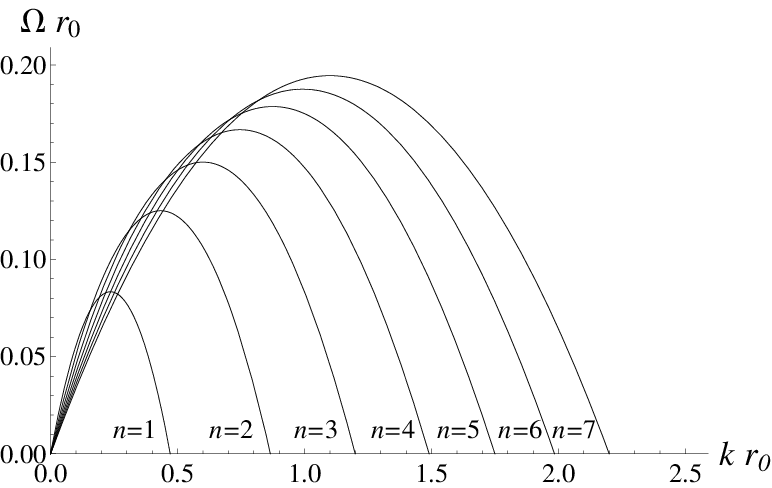
which is valid up to corrections . Figure 1 compares this dispersion relation to the numerical results obtained from linearized perturbations of a black -brane.

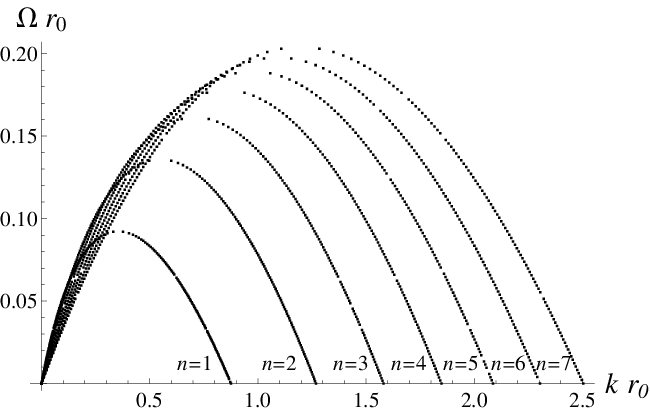
Zooming in on small values of , the match is excellent. When is of order one we have no right to expect agreement, but the overall qualitative resemblance of the curves is nevertheless striking. The quantitative agreement improves with increasing and indeed, as figure 2 shows, at large it becomes impressively good over all wavelengths: for the numerical values are reproduced to better than accuracy up to the maximum value of . Although the extent of this agreement is surprising, we will provide some arguments for why the fluid approximation appears to be so successful as grows.
Thus, the effective viscous fluid seems to capture in a simple manner some of the most characteristic features of black brane dynamics. We believe this is a significant simplification from the complexity of the full Einstein equations.
The outline of the rest of the paper is as follows: the next section contains the bulk of the calculations of the paper for a generic hydrodynamic-type perturbation of the black brane. We highlight the differences with the analysis of [2], in particular at asymptotic infinity, and compute the values (1.3) for the effective and . Section 3 relates the linearized damped sound-mode perturbations of the fluid to the Gregory-Laflamme perturbations of the black brane. We examine the conditions that can lead to the surprising quantitative agreement of the dispersion relation at large , and we propose its exact form as . We close in section 4 with an examination of the differences with other fluid-like approaches to the GL instability, and a discussion of our results within the context of the blackfold approach.
2 Hydrodynamic perturbations of black branes
In this section we study general perturbations of a vacuum black -brane with slow variation along the worlvolume directions of the brane. Up to gauge transformations, they are fully determined by the boundary conditions of horizon regularity and asymptotic flatness at spatial infinity. Most of our analysis is very close to the study of hydrodynamic perturbations of AdS black branes, but there is an additional complication in the study of the perturbations at asymptotic infinity. Nevertheless, we are able to find the complete explicit form of the perturbed solution for a generic hydrodynamic flow to first order in the derivative expansion.
Readers who do not need or want the technical details of the calculation of the perturbed solution and the viscous stress tensor can safely skip to section 3.
2.1 Preliminaries
2.1.1 Black branes and their effective stress tensor
The black -brane solution of vacuum gravity in dimensions is
| (2.1) |
with . The solution is characterized by the horizon radius (or brane ‘thickness’) and the worldvolume velocity , with . It is asymptotically flat in the directions transverse to the worldvolume coordinates . We can associate to it a stress-energy tensor measured at spatial infinity. There are several possible definitions of this stress tensor that would be equivalent for calculational purposes, but for conceptual reasons the most convenient for us is the quasilocal one of Brown and York [12]. We consider a boundary surface at large constant , with induced metric and compute
| (2.2) |
where is the extrinsic curvature of the surface and we perform a background substraction from flat spacetime.
The geometry of the boundary surface for (2.1) is . We will introduce perturbations with wavelengths much longer than the size of the at the horizon. The deformations of this sphere all have large masses and therefore decouple. Thus the symmetry of is preserved and, in an appropriate gauge, the metric will remain a direct product with a factor of this sphere. We integrate over the sphere to obtain the stress tensor for the black -brane
| (2.3) |
We regard this stress tensor as living on the worldvolume of the brane, i.e., the extended directions of the boundary. The worldvolume metric results from the asymptotic form of the boundary metric, which in our case is the Minkowski metric
| (2.4) |
A main advantage of using the quasilocal stress tensor is that the Gauss-Codacci equations for the constant- cylinder imply , so imposing the Einstein equations in vacuum it follows that the stress tensor is conserved
| (2.5) |
The stress tensor for the solution (2.1) has the perfect fluid form
| (2.6) |
with energy density and pressure
| (2.7) |
The horizon area allows to associate a local entropy density to this effective fluid
| (2.8) |
and all the thermodynamic functions can be expressed as functions of the temperature
| (2.9) |
We can equivalently use or as the variable that determines local equilibrium. In this section we will mostly use for notational simplicity.
We will be interested in preserving regularity at the horizon. This is manifest if instead of the Schwarzschild coordinates in (2.1) we use Eddington-Finkelstein (EF) ones,
| (2.10) |
such that
| (2.11) |
2.1.2 Perturbations
We promote the thickness and velocity parameters to collective fields over the worldvolume, so
| (2.12) | |||||
where and are assumed to vary slowly relative to the scale set by . In this paper we expand them to first order in derivatives, which we keep track of through a formal derivative-counting parameter . With non-uniform and , the metric (2.12) is not Ricci flat so we add to it a component with radial dependence
| (2.13) |
We choose a gauge in which is a null vector with normalization fixed by the radius of , so that
| (2.14) |
With this choice the sphere can be integrated out.
Demanding that (2.13) satisfies the vacuum Einstein equations to first order in results into a set of ODEs for . These will be solved subject to regularity at the horizon , which is easily imposed as a condition of metric finiteness in EF coordinates, and to asymptotic flatness, to which we turn next.
2.1.3 Asymptotic infinity
The asymptotic behavior of our spacetimes introduces an important difference relative to the perturbations of AdS black branes. For the latter, the calculations can be performed in their entirety in EF coordinates in which is a null vector. By taking large values of in these coordinates one approaches null infinity, but in AdS this is the same as spatial infinity. The AdS boundary is always a timelike surface. However, in our asymptotically flat space, null and spatial infinities differ.
We are ultimately interested in computing the quasilocal stress tensor on a timelike boundary of spacetime endowed with a non-degenerate metric. But if we approach null infinity, the boundary metric will be degenerate and it is unclear whether the quasilocal stress tensor is well defined there. Instead, it seems more appropriate (and is definitely unproblematic) to compute the stress tensor at spatial infinity44 4 Presumably the appropriate notion of spatial infinity here is not Penrose’s (which is just a point) but more along the lines of [13], which naturally allows a dependence along the boundary directions. Although our spatial infinity is not exactly the same as in [13] since instead of a hyperboloid we work on a cylinder where and scale differently at infinity, this is not a problem for us since we are integrating over . It would be interesting, especially with a view to holography, to further formalize this notion of spatial infinity. Related remarks concerning holography in asymptotically flat spacetimes have been made in [14].. For this purpose EF coordinates are very awkward and it is much more convenient to switch back to Schwarzschild-like coordinates at large .
Thus we will work with two sets of coordinates: EF ones, in which horizon regularity is manifest, and Schwarzschild coordinates, in which spatial infinity is naturally approached. We need to provide the change of coordinates that relates them, extending the inverse of (2.10) to include terms. The correction is naturally guessed by recalling that and , which appear in the transformation (2.10), now depend on the EF coordinates. Thus,
| (2.15) |
or more explicitly,
| (2.16) |
2.2 Solving the perturbation equations
At each point we choose coordinates centered on that point and go to an (unperturbed) local rest frame. In EF coordinates the velocity perturbation is
| (2.17) |
Note that since local velocities are small the constraint is automatically satisfied to the order we need. The other collective variable of the effective black brane fluid is the temperature , or equivalently the thickness , which we perturb as
| (2.18) |
In the following we understand all quantities as evaluated at and thus denote , etc.
The Einstein equations with a radial index, do not involve second derivatives and are constraint equations. Indeed they only involve the hydrodynamic fields and and not ,
| (2.21) |
so they are to be regarded as the equations of fluid dynamics, consistently with (2.5). We also verify this interpretation later.
The remaining Einstein’s equations are dynamical and we solve them to find . The equations give
| (2.22) |
which, requiring finiteness at the horizon, are solved by
| (2.23) |
The integration constants will be fixed later demanding asymptotic flatness. The equations ,
| (2.24) |
are solved by
| (2.25) |
which are regular at the horizon for all values of the constants. Next, the equations from and are
| (2.26) |
and
| (2.27) |
which, assuming that eqs. (2.21) are satisfied, are solved by
| (2.28) |
and
| (2.29) |
Again these are regular at the horizon for all choices of the integration constants. Note that does not appear in Einstein’s equations to first order in and corresponds to a gauge mode. This, and the integration constants, will be fixed shortly.
At this stage, for any hydrodynamic perturbation that solves the equations (2.21), we have managed to construct a perturbed metric that is regular at the horizon. Next we must ensure that the solution remains asymptotically flat. Transforming to Schwarzchild-like coordinates using (2.16), we require that
| (2.30) |
For the other metric components, we find that , , and when ( when ), are enough to obtain a finite stress tensor. Recall also that all the metric components involving angular coordinates of are unaltered.
Omitting details, we find that the conditions on and fix
| (2.31) |
In addition, the effect of in amounts to a global shift in the velocity field along the spatial directions of the brane, so in order to remain in a local rest frame we set
| (2.32) |
Furthermore, if we perform the change
| (2.33) |
then results in a global shift in the temperature, which we eliminate by choosing
| (2.34) |
Asymptotic flatness in imposes a choice for that singles out the slower fall-off of ,
| (2.35) |
(note that the values of and at are equal).
Asymptotic flatness in these coordinates is a little delicate when due to its slower fall-off, and to make it manifest we take an gauge diverging at infinity. This is not necessary when (and neither choice affects the calculation of the stress tensor). Thus we set
| (2.36) |
Summarizing, we obtain
| (2.37) | ||||
| (2.38) | ||||
| (2.39) | ||||
| (2.40) | ||||
| (2.41) | ||||
| (2.42) |
( correspond to Schwarzschild coordinates here, so ). This is the complete solution for the black brane metric that corresponds to a hydrodynamic perturbation that solves the equations (2.21) expanded around the origin of the local rest frame, .
2.3 Viscous stress tensor
We are now ready to compute the quasilocal stress tensor (2.2). The renormalization via background subtraction is simple and appropriate, since our metrics are infinitesimally close to the uniform black -brane and their asymptotic boundaries can always be embedded in flat spacetime. Straightforward calculations give
| (2.43) | |||||
which are valid up to . One can easily check that the hydrodynamic equations are indeed equivalent to the constraint equations (2.21).
Write now this stress tensor in the form
| (2.44) |
where the expansion and shear of the velocity congruence are
| (2.45) |
3 Damped unstable sound waves and the Gregory-Laflamme instability
Our analysis in the previous section applies to generic long-wavelength perturbations of arbitrarily large amplitude. Let us now consider small perturbations of a static fluid of the form
| (3.1) |
where is the speed of sound, and with
| (3.2) |
We substitute these in the viscous fluid equations and linearize in the amplitudes and , to find
| (3.3) | |||||
| (3.4) |
Applying our results above, any solution to these equations can be used to obtain an explicit black brane solution with a small, long-wavelength fluctuation of and . If we eliminate we find that non-trivial sound waves require
| (3.5) |
where and we have used the Gibbs-Duhem relation . This equation determines the dispersion relation . For a stable fluid with , viscosity adds a small imaginary part to the frequency, which becomes complex and describes damped sound oscillations. Instead our effective fluid has imaginary sound-speed, eq. (1.4), so is purely imaginary: sound waves are unstable. Writing
| (3.6) |
we solve (3.5) to find
| (3.7) |
For the specific black -brane fluid this yields the dispersion relation (1.5). The connection between these unstable sound waves and the Gregory-Laflamme instability was pointed out at the perfect fluid level (i.e., linear in ) in [3], and we have discussed it in the introduction.55 5 Observe that the result (1.5) is independent of . That this must be the case is clear from the outset in the GL analysis and also in our analysis of the Einstein equations.
Figures 1 and 2 show that our approximation (1.5) improves as grows. In order to see how this might be justified, let us first rewrite the dispersion relation (1.5) in terms of the temperature instead of ,
| (3.8) |
In principle, at any given , both quantities and define length scales that are parametrically equivalent. But if we vary and allow it to take large values, then and can differ greatly. We propose that in this case, , and not , is the length scale that limits the validity of the fluid approximation, so the appropriate expansion variable for large is and not . This may actually be natural since from the fluid point of view has a clearer physical meaning than . In effect, we are proposing that when it is more accurate to view the effective theory as describing very hot black branes, rather than very thin ones.
The point of this exercise is that for large the maximum values over which and in (3.8) range are and . So as grows the frequency and wavenumber of unstable modes extend over a smaller range of and . This strongly suggests that hydrodynamics can capture more accurately the dynamics of GL modes when the number of dimensions becomes very large.66 6 This is similar in spirit, although not precisely equal, to the proposal in [15] that in the limit of large number of dimensions black holes are accurately described by fluid mechanics. More precisely, if we write the corrections inside the brackets in (3.8) in the form , and assume that the -dependence of the coefficients is such that as , then the expansion in , i.e., the hydrodynamic derivative expansion, becomes a better approximation over a larger portion of the curves .
This is a relatively mild-looking assumption on the -dependence of the higher-order coefficients in the expansion in ,77 7 Which, crucially, is not satisfied by the coefficient of the linear term inside the brackets in (3.8). and in particular is satisfied if the remain finite as . But since we have not computed higher-derivative transport coefficients then, within our perturbative framework, we cannot prove its validity. However, since the numerical data appear to strongly support it, we conjecture that the truncation of the dispersion relation up to -terms captures the complete dispersion relation at large . More precisely, if we define a rescaled frequency and wavenumber,
| (3.9) |
that remain finite as , then we propose that
| (3.10) |
is the exact limiting relation valid for all wavenumbers .
Note that the truncation of in (3.8) appears to capture the zero-mode with at a finite . This is quite remarkable, since the viscous fluid equation (3.5) does not admit any zero-mode solution. The comparison with numerical data in figure 2 shows that the quantitative result for , although poor for small , becomes excellent for large . Further evidence for the validity of our proposal comes from the analytical value of the GL zero mode in the limit [16]
| (3.11) |
This is the same as the limiting value for the zero-mode ‘predicted’ by (3.9), (3.10).88 8 The relative difference between the results for from the large- subleading correction computed in [17] and from (1.5) is equal to . This is precisely the size of the discrepancy observed in fig. 2.
4 Discussion
Our analysis of the GL instability must not be confused with recent studies where a connection to the Rayleigh-Plateau instability of fluid tubes is made. In the latter approach, following a suggestion in [18], refs. [15, 19] related a -dimensional black string in a Scherk-Schwarz compactification of Anti-deSitter space to a -dimensional fluid tube with a boundary with surface tension (see [20]). The Rayleigh-Plateau instability of the fluid tube arises from the competition between surface tension and bulk pressure. In contrast, our effective fluid does not have any boundaries so the instability is not of the Rayleigh-Plateau type, but rather one in the sound modes. Also note that our calculations in sec. 2 yield explicit black brane solutions to the Einstein equations (in vacuum) in a derivative expansion, something that, although expected to be possible in principle, at present cannot be realized for the fluid solutions in [15, 19].
We stress that our analysis is not a ‘dual’ solution of the GL instability problem: we have investigated the same perturbation problem as in [10] and explicitly solved it in closed analytic form in a derivative expansion. Since our approach does not require the perturbations to be small, it may even be used to study the non-linear evolution of the GL instability.
One of our motivations has been to show explicitly how the effective theory of blackfolds of [3] can be systematically developed as a derivative expansion of the Einstein equations. Although we have done it only for the intrinsic aspects of blackfold dynamics, we have been able to: (i) derive in detail, starting from the ‘microscopic’ (full Einstein) theory, the lowest-order blackfold formalism that ref. [3] had developed following general principles; (ii) prove that the first corrections to the lowest-order formalism can be computed and result in perturbations of the black brane that preserve regularity of the horizon. The viscosity coefficients are determined precisely from this condition.
In general, the worldvolume of a blackfold is dynamical and can be curved. Our calculations in this paper can be regarded as being valid for fluid perturbations with a wavelength that, while longer than , is much shorter than the typical curvature radius of the blackfold worldvolume. In this case, the intrinsic and extrinsic dynamics decouple. Thus, for a curved blackfold our results for the GL instability are valid at most up to wavelengths smaller than . At longer wavelengths the hydrodynamics of the effective fluid is fully coupled to the elastic dynamics of the worldvolume. For instance this is case for perturbations of thin black rings with wavelength comparable to the ring radius. These lie beyond the range of applicability of our results.
It should be quite interesting to extend our analysis to include the extrinsic aspects of the blackfold. To do this, one first allows the worldvolume metric where the fluid lives to be a curved background, with an extrinsic curvature radius much larger than . This curvature acts as an external force on the fluid [3]. In the derivative expansion, the stress tensor will in general contain, besides the viscosities, higher-derivative coefficients that multiply derivatives of the worldvolume metric. These coefficients will be determined by demanding horizon regularity of a perturbation that curves the asymptotic geometry. Perturbations of this kind have been studied for certain illustrative examples in [21, 22, 5] in stationary situations that do not involve viscous dissipation. Thus it may be possible to extract the extrinsic pressure coefficients in the stress tensor.
In the AdS context, the external force on the fluid from a worldvolume curvature has been studied in [23]. However, in that case the worldvolume geometry is regarded as a fixed, non-dynamical background. Instead, in the blackfold context this geometry is dynamical. A solution of the forced fluid equations will backreact on the background spacetime where the blackfold lives, and thus modify the worldvolume geometry. Therefore for a generic, curved blackfold the explicit construction of perturbative metrics becomes rather more complicated than in the fluid/AdS-gravity correspondence.
Acknowledgments
We are indebted to Pau Figueras for kindly providing the excellent numerical data for the Gregory-Laflamme instability used in figures 1 and 2. We thank Troels Harmark, Vasilis Niarchos, and Niels Obers for discussions. JC thanks the NBI for warm hospitality. Work supported by DURSI 2009 SGR 168, MEC FPA 2007-66665-C02 and CPAN CSD2007-00042 Consolider-Ingenio 2010. JC was also supported in part by FPU grant AP2005-3120.
References
- [1] T. Damour, “Surface Effects in Black Hole Physics”, Proceedings of the Second Marcel Grossmann Meeting on General Relativity, (edited by R. Ruffini, North Holland, 1982) p. 587. K. S. Thorne, R. H. Price and D. A. Macdonald, “Black Holes: The Membrane Paradigm”, Yale Univ. Press, New Haven, USA (1986).
- [2] S. Bhattacharyya, V. E. Hubeny, S. Minwalla and M. Rangamani, “Nonlinear Fluid Dynamics from Gravity,” JHEP 0802 (2008) 045 [arXiv:0712.2456 [hep-th]].
- [3] R. Emparan, T. Harmark, V. Niarchos and N. A. Obers, “Essentials of Blackfold Dynamics,” JHEP 1003 (2010) 063 [arXiv:0910.1601 [hep-th]].
- [4] R. Emparan, T. Harmark, V. Niarchos and N. A. Obers, “Worldvolume Effective Theory for Higher-Dimensional Black Holes (Blackfolds),” Phys. Rev. Lett. 102, 191301 (2009) [arXiv:0902.0427 [hep-th]].
- [5] R. Emparan, T. Harmark, V. Niarchos and N. A. Obers, “New Horizons for Black Holes and Branes,” arXiv:0912.2352 [hep-th].
- [6] P. Kovtun, D. T. Son and A. O. Starinets, “Viscosity in strongly interacting quantum field theories from black hole physics,” Phys. Rev. Lett. 94 (2005) 111601 [arXiv:hep-th/0405231].
- [7] A. Buchel, “Bulk viscosity of gauge theory plasma at strong coupling,” Phys. Lett. B 663, 286 (2008) [arXiv:0708.3459 [hep-th]].
- [8] N. Iqbal and H. Liu, “Universality of the hydrodynamic limit in AdS/CFT and the membrane paradigm,” Phys. Rev. D 79 (2009) 025023 [arXiv:0809.3808 [hep-th]].
- [9] M. Fujita, “Non-equilibrium thermodynamics near the horizon and holography,” JHEP 0810 (2008) 031 [arXiv:0712.2289 [hep-th]].
- [10] R. Gregory and R. Laflamme, “Black strings and p-branes are unstable,” Phys. Rev. Lett. 70 (1993) 2837 [arXiv:hep-th/9301052]; “The Instability of charged black strings and p-branes,” Nucl. Phys. B 428 (1994) 399 [arXiv:hep-th/9404071].
- [11] A. Buchel, “A holographic perspective on Gubser-Mitra conjecture,” Nucl. Phys. B 731 (2005) 109 [arXiv:hep-th/0507275].
- [12] J. D. Brown and J. W. York, “Quasilocal energy and conserved charges derived from the gravitational action,” Phys. Rev. D 47 (1993) 1407 [arXiv:gr-qc/9209012].
- [13] A. Ashtekar and J. D. Romano, “Spatial infinity as a boundary of space-time,” Class. Quant. Grav. 9 (1992) 1069.
- [14] D. Marolf, “Asymptotic flatness, little string theory, and holography,” JHEP 0703, 122 (2007) [arXiv:hep-th/0612012].
- [15] M. M. Caldarelli, O. J. C. Dias, R. Emparan and D. Klemm, “Black Holes as Lumps of Fluid,” JHEP 0904 (2009) 024 [arXiv:0811.2381 [hep-th]].
- [16] B. Kol and E. Sorkin, “On black-brane instability in an arbitrary dimension,” Class. Quant. Grav. 21 (2004) 4793 [arXiv:gr-qc/0407058].
- [17] V. Asnin, D. Gorbonos, S. Hadar, B. Kol, M. Levi and U. Miyamoto, “High and Low Dimensions in The Black Hole Negative Mode,” Class. Quant. Grav. 24 (2007) 5527 [arXiv:0706.1555 [hep-th]].
- [18] V. Cardoso and O. J. C. Dias, “Gregory-Laflamme and Rayleigh-Plateau instabilities,” Phys. Rev. Lett. 96, 181601 (2006) [arXiv:hep-th/0602017].
- [19] K. i. Maeda and U. Miyamoto, “Black hole-black string phase transitions from hydrodynamics,” JHEP 0903, 066 (2009) [arXiv:0811.2305 [hep-th]].
- [20] O. Aharony, S. Minwalla and T. Wiseman, “Plasma-balls in large N gauge theories and localized black holes,” Class. Quant. Grav. 23 (2006) 2171 [arXiv:hep-th/0507219].
- [21] R. Emparan, T. Harmark, V. Niarchos, N. A. Obers and M. J. Rodriguez, “The Phase Structure of Higher-Dimensional Black Rings and Black Holes,” JHEP 0710 (2007) 110 [arXiv:0708.2181 [hep-th]].
- [22] M. M. Caldarelli, R. Emparan and M. J. Rodriguez, “Black Rings in (Anti)-deSitter space,” JHEP 0811, 011 (2008) [arXiv:0806.1954 [hep-th]].
- [23] S. Bhattacharyya, R. Loganayagam, S. Minwalla, S. Nampuri, S. P. Trivedi and S. R. Wadia, “Forced Fluid Dynamics from Gravity,” JHEP 0902 (2009) 018 [arXiv:0806.0006 [hep-th]].