Evidence for direct $CP$ violation in the decay $B^{\pm}\to D^{(*)}K^{\pm}$, $D\to K^{0}_{S}\pi^{+}\pi^{-}$ and measurement of the CKM phase $\phi_{3}$

Determinations of parameters of the Cabibbo-Kobayashi-Maskawa (CKM) matrix [1] are important as checks on the consistency of the Standard Model, and as ways to search for new physics. Among the angles of the CKM unitarity triangle, $\phi_{3}$ (also widely known as $\gamma$) is the least-well constrained by direct measurements, so new results are of particular interest. The principal experimental resource is $CP$ violation in the family of decays $B\to DK$: various methods for extracting a $\phi_{3}$ measurement have been proposed [2, 3, 4, 5], following the original discussion of direct $CP$ violation measurement by Bigi, Carter, and Sanda [6]. The most sensitive technique relies on three-body final states [7, 8] such as $K^{0}_{S}\pi^{+}\pi^{-}$.

In the Wolfenstein parameterization of the CKM matrix elements [9], the weak parts of the amplitudes that contribute to the decay $B^{+}\to DK^{+}$ are given by $V_{cb}^{*}V_{us\vphantom{b}}^{\vphantom{*}}\sim A\lambda^{3}$ (for the $\overline{D}{}^{0}K^{+}$ final state) and $V_{ub}^{*}V_{cs\vphantom{b}}^{\vphantom{*}}\sim A\lambda^{3}(\rho+i\eta)$ (for $D^{0}K^{+}$); the two amplitudes interfere as the $D^{0}$ and $\overline{D}{}^{0}$ mesons decay into the same final state $K^{0}_{S}\pi^{+}\pi^{-}$. Assuming no $CP$ asymmetry in neutral $D$ decays, the amplitude for the process $B^{\pm}\to(K^{0}_{S}\pi^{+}\pi^{-})_{D}K^{\pm}$ as a function of the Dalitz plot variables $m^{2}_{+}=m^{2}_{K^{0}_{S}\pi^{+}}$ and $m^{2}_{-}=m^{2}_{K^{0}_{S}\pi^{-}}$ is

where $f(m^{2}_{+},m^{2}_{-})$ is the amplitude of the $\overline{D}{}^{0}\to K^{0}_{S}\pi^{+}\pi^{-}$ decay, $r$ is the ratio of the magnitudes of the two interfering amplitudes, and $\delta$ is the strong phase difference between them. The $\overline{D}{}^{0}\to K^{0}_{S}\pi^{+}\pi^{-}$ decay amplitude $f$ can be determined from a large sample of flavor-tagged $\overline{D}{}^{0}\to K^{0}_{S}\pi^{+}\pi^{-}$ decays produced in continuum $e^{+}e^{-}$ annihilation. Once $f$ is known, a simultaneous fit to $B^{+}$ and $B^{-}$ data allows the contributions of $r$, $\phi_{3}$ and $\delta$ to be separated. The method has a two-fold ambiguity: $(\phi_{3},\delta)$ and $(\phi_{3}+180{}^{\circ},\delta+180{}^{\circ})$ solutions cannot be separated. We always choose the solution with $0<\phi_{3}<180{}^{\circ}$. We neglect the effects of charm mixing in this formalism. Given the current precision of $\phi_{3}$ and the constraints on the $D^{0}$ mixing parameters ($x_{D},y_{D}\sim 0.01$ [10]), these effects can be safely neglected [11], although it is possible to take them into account if they appear to be significant for future precision measurements. References [7] and [12] give a more detailed description of the technique.

This method can be applied to other decay modes: in addition to $B^{+}\to DK^{+}$,¹¹ 1 Charge-conjugate modes are implied throughout the paper unless noted otherwise. excited states of neutral $D$ and $K$ can also be used, although the values of $\delta$ and $r$ can differ for these decays. Both the BaBar and Belle collaborations have successfully applied this technique to $B^{\pm}\to D^{(*)}K^{(*)\pm}$ modes with $D^{0}$ decaying to $K^{0}_{S}\pi^{+}\pi^{-}$ [15, 16, 13, 14, 12]. In addition, the BaBar collaboration reported a measurement of $\phi_{3}$ using the $B^{\pm}\to DK^{\pm}$ mode with the $D$ decaying to the $K^{0}_{S}K^{+}K^{-}$ [16] and $\pi^{0}\pi^{+}\pi^{-}$ [17] final states.

Here we present a measurement of $\phi_{3}$ using the modes $B^{+}\to DK^{+}$ and $B^{+}\to D^{*}K^{+}$ with $D\to K^{0}_{S}\pi^{+}\pi^{-}$, based on a 605 fb^-1 data sample ($657\times 10^{6}$ $B\overline{B}$ pairs) collected by the Belle detector at the KEKB asymmetric $e^{+}e^{-}$ collider. The Belle detector is described in detail elsewhere [18, 19]. It is a large-solid-angle magnetic spectrometer consisting of a silicon vertex detector (SVD), a 50-layer central drift chamber (CDC) for charged particle tracking and specific ionization measurement ($dE/dx$), an array of aerogel threshold Cherenkov counters (ACC), time-of-flight scintillation counters (TOF), and an array of CsI(Tl) crystals for electromagnetic calorimetry (ECL) located inside a superconducting solenoid coil that provides a 1.5 T magnetic field. An iron flux return located outside the coil is instrumented to detect $K_{L}$ mesons and identify muons (KLM).

The results presented in this paper supersede our previous measurement based on a sample of $386\times 10^{6}$ $B\overline{B}$ pairs [12]. In addition to $B^{\pm}\to DK^{\pm}$ and the $B^{\pm}\to D^{*}K^{\pm}$ mode with $D^{*}\to D\pi^{0}$, this analysis exploits $B^{\pm}\to D^{*}K^{\pm}$ with $D^{*}\to D\gamma$. The $D^{*}\to D\gamma$ mode has nearly the same parameters as $B^{\pm}\to D^{*}K^{\pm}$ with $D^{*}\to D\pi^{0}$, the only difference being that due to the opposite $C$ parities of the $\gamma$ and $\pi^{0}$, the strong phases for these modes differ by $180^{\circ}$ [20]. This provides an additional cross-check for the analysis and allows systematic uncertainties in the combined measurement to be reduced. The analysis procedure is also improved. It uses additional variables in the maximum likelihood fit for the separation of signal from background; this allows one to relax some selection requirements, thus increasing the sample size.

The decay chains $B^{+}\to DK^{+}$ and $B^{+}\to D^{*}K^{+}$ with $D^{*}\to D\pi^{0}$ and $D^{*}\to D\gamma$ are selected for the analysis. The neutral $D$ meson is reconstructed in the $K^{0}_{S}\pi^{+}\pi^{-}$ final state in all cases. We also select decays $D^{*-}\to\overline{D}{}^{0}\pi^{-}$ produced via the $e^{+}e^{-}\to c\bar{c}$ continuum process as a high-statistics sample to determine the $\overline{D}{}^{0}\to K^{0}_{S}\pi^{+}\pi^{-}$ decay amplitude.

Charged tracks are required to satisfy criteria based on the quality of the track fit and the distance from the interaction point. We require each track to have a transverse momentum greater than 100 MeV/$c$. (The reference axis is given by the direction of the $e^{+}$ beam.) Separation of kaons and pions is accomplished by combining the responses of the ACC and the TOF with the $dE/dx$ measurement from the CDC. Photon candidates are required to have ECL energy greater than 30 MeV. Neutral pion candidates are formed from pairs of photons with invariant masses in the range 120 MeV/$c^{2}$ to 150 MeV/$c^{2}$. Neutral kaons are reconstructed from pairs of oppositely charged tracks with an invariant mass $M_{\pi\pi}$ within $7$ MeV/$c^{2}$ of the nominal $K^{0}_{S}$ mass, and forming a vertex more than 1 mm from the interaction point in the transverse plane.

To determine the $\overline{D}{}^{0}\to K^{0}_{S}\pi^{+}\pi^{-}$ decay amplitude we use $D^{*\pm}$ mesons produced via the $e^{+}e^{-}\to c\bar{c}$ continuum process. The flavor of the neutral $D$ meson is tagged by the charge of the slow pion (which we denote as $\pi_{s}$) in the decay $D^{*-}\to\overline{D}{}^{0}\pi_{s}^{-}$. The slow pion track is fitted to the $\overline{D}{}^{0}$ production vertex to improve the momentum and angular resolution of the $\pi_{s}$. To select neutral $D$ candidates we require the invariant mass of the $K^{0}_{S}\pi^{+}\pi^{-}$ system to be within 11 MeV/$c^{2}$ of the $D^{0}$ mass. To select events originating from a $D^{*-}$ decay we impose a requirement on the difference $\Delta M$ of the invariant masses of the $D^{*-}$ and the neutral $D$ candidates: $144.9\mbox{ MeV}/c^{2}<\Delta M<145.9\mbox{ MeV}/c^{2}$. Suppression of the combinatorial background from $B\overline{B}$ events is achieved by requiring the $D^{*-}$ momentum in the center-of-mass (CM) frame to be greater than 3.0 GeV/$c$. The number of events in the signal region is $290.9\times 10^{3}$; the background fraction is 1.0%.

The selection of $B$ candidates is based on the CM energy difference $\Delta E=\sum E_{i}-E_{\rm beam}$ and the beam-constrained $B$ meson mass $M_{\rm bc}=\sqrt{E_{\rm beam}^{2}-(\sum\vec{p}_{i})^{2}}$, where $E_{\rm beam}$ is the CM beam energy, and $E_{i}$ and $\vec{p}_{i}$ are the CM energies and momenta of the $B$ candidate decay products. We select events with $M_{\rm bc}>5.2$ GeV/$c^{2}$ and $|\Delta E|<0.15$ GeV for further analysis. We also impose a requirement on the invariant mass of the neutral $D$ candidate as above: $|M_{K^{0}_{S}\pi^{+}\pi^{-}}-M_{D^{0}}|<11$ MeV/$c^{2}$. To obtain the Dalitz plot variables $m^{2}_{+}$ and $m^{2}_{-}$, a kinematical fit is employed with the constraint that the $K^{0}_{S}\pi^{+}\pi^{-}$ invariant mass be equal to $M_{D^{0}}$.

We consider two major background sources in our data: the continuum process $e^{+}e^{-}\to q\bar{q}$, where the light component with $q=u,d,s$ and the charmed component are treated separately; and $B\overline{B}$ decays, where events with real $D^{0}$ (due to $B^{\pm}\to D\pi^{\pm}$ etc.) are treated separately. To suppress background from continuum events, we calculate two variables that characterize the event shape. One is the cosine of the thrust angle $\cos\theta_{\rm thr}$, where $\theta_{\rm thr}$ is the angle between the thrust axis of the $B$ candidate daughters and that of the rest of the event, calculated in the CM frame. The other is a Fisher discriminant $\mathcal{F}$ composed of 11 parameters [21]: the production angle of the $B$ candidate, the angle of the $B$ thrust axis relative to the beam axis, and nine parameters representing the momentum flow in the event relative to the $B$ thrust axis in the CM frame. In the first stage of the analysis, the $(M_{\rm bc},\Delta E)$ distribution is fitted in order to obtain the fractions of the background components, and we require $|\cos\theta_{\rm thr}|<0.8$ and $\mathcal{F}>-0.7$. In the Dalitz plot fit, we do not reject events based on these variables (as in the previous analysis [12]), but rather use them in the likelihood function to better separate signal and background events. This leads to a 7–8% improvement in the expected statistical error.

The $\Delta E$ and $M_{\rm bc}$ distributions for the $B^{+}\to DK^{+}$ mode are shown in Fig. 1 (a), (b). For the selected events a two-dimensional unbinned maximum likelihood fit in the variables $M_{\rm bc}$ and $\Delta E$ is performed, with the fractions of continuum, $B\bar{B}$ and $B^{\pm}\to D^{(*)}\pi^{\pm}$ backgrounds as free parameters, and their distributions fixed from generic MC simulation. (The continuum component is also split into $(u,d,s)$ and charm components in the figure, based on fractions in the MC.) The resulting signal and background fractions are used in the Dalitz plot fit to obtain the event-by-event signal to background ratio. A more detailed description of the two-stage procedure is given in Section IV. The number of events in the signal box ($M_{\rm bc}>5.27$ GeV/$c^{2}$, $|\Delta E|<30$ MeV, $|\cos\theta_{\rm thr}|<0.8$, $\mathcal{F}>-0.7$) is 756, with a signal purity of $(70.5\pm 1.2)$%. The $(M_{\rm bc},\Delta E)$ fit yields a continuum background fraction of $(17.9\pm 0.7)$%, a $B\overline{B}$ background fraction of $(7.3\pm 0.5)$%, and a $B^{\pm}\to D\pi^{\pm}$ background fraction of $(4.3\pm 0.3)$% in the signal box. Figure 2 shows the distributions of $\cos\theta_{\rm thr}$ and $\mathcal{F}$ variables in the $M_{\rm bc}$, $\Delta E$ signal region for the $B^{+}\to DK^{+}$ mode. The distributions for the other modes are similar.

To select $B^{+}\to D^{*}K^{+}$ events with $D^{*}\to D\pi^{0}$, in addition to the requirements described above, we require that the mass difference $\Delta M$ of neutral $D^{*}$ and $D$ candidates satisfies $140\mbox{ MeV}/c^{2}<\Delta M<144\mbox{ MeV}/c^{2}$. The $\Delta E$ and $M_{\rm bc}$ distributions for this mode are shown in Fig. 1 (c), (d). The background fractions are obtained in the same way as for $B^{\pm}\to DK^{\pm}$ mode. The number of events in the signal box is 149, with $(79.7\pm 2.5)$% signal purity. The continuum background fraction is $(5.7\pm 0.7)$%, the $B\overline{B}$ background fraction is $(7.6\pm 1.9)$%, and the $B^{\pm}\to D^{*}\pi^{\pm}$ background fraction is $(7.0\pm 1.3)$%.

Selection of the $B^{+}\to D^{*}K^{+}$ mode with $D^{*}\to D\gamma$ is performed in a similar way. The photon candidate is required to have an energy greater than 100 MeV, and the mass difference requirement is $\Delta M<152$ MeV$/c^{2}$. Due to the larger number of background sources for this mode, the treatment of background differs. The $B\overline{B}$ background is subdivided into events with combinatorial $D$, studied using a generic MC sample; and those with real neutral $D$ mesons, for which a dedicated simulation of each component is performed. The fractions of background components are obtained from an unbinned 4D fit of the distribution of variables $M_{\rm bc}$, $\Delta E$, $\cos\theta_{\rm thr}$, and $\mathcal{F}$. The relative fractions of $B\overline{B}$ backgrounds with a real $D^{0}$ (except for $B^{\pm}\to D^{*}\pi^{\pm}$ and $B^{\pm}\to DK^{\pm}$) are fixed according to their PDG branching ratios [22] and MC efficiencies. The $\Delta E$ and $M_{\rm bc}$ distributions for this mode are shown in Fig. 1 (e), (f). The number of events in the signal box is 141, and the signal purity is $(41.7\pm 3.6)$%. The continuum background fraction is $(15.8\pm 1.3)$%, the fraction of $B\overline{B}$ background with combinatorial $D^{0}$ is $(21.3\pm 3.0)$%, the contribution of $B^{\pm}\to D^{*}\pi^{\pm}$, $D^{*}\to D\gamma$ is $(6.5\pm 1.2)$%, and the fraction of the rest of $B\overline{B}$ events with real $D^{0}$ is $(14.7\pm 1.1)$%.

The Dalitz distributions of $D\to K^{0}_{S}\pi^{+}\pi^{-}$ decay in the signal box for each of the $B^{\pm}\to DK^{\pm}$ and $B^{\pm}\to D^{*}K^{\pm}$ processes are shown in Fig. 3.

As in our previous analysis [12], the $\overline{D}{}^{0}\to K^{0}_{S}\pi^{+}\pi^{-}$ decay amplitude is represented using the isobar model. The list of resonances is also the same, the only difference being the free parameters (mass and width) of the $K^{*}(892)^{\pm}$ and $\rho(770)$ states. A modified amplitude, where the scalar $\pi\pi$ component is described using the K-matrix approach [23], is used in the estimation of the systematic error.

The amplitude $f$ for the $\overline{D}{}^{0}\to K^{0}_{S}\pi^{+}\pi^{-}$ decay is described by a coherent sum of $N$ two-body decay amplitudes and one non-resonant decay amplitude,

where $\mathcal{A}_{j}(m^{2}_{+},m^{2}_{-})$ is the matrix element, $a_{j}$ and $\xi_{j}$ are the amplitude and phase of the matrix element, respectively, of the $j$-th resonance, and $a_{\text{NR}}$ and $\xi_{\text{NR}}$ are the amplitude and phase of the non-resonant component. The description of the matrix elements follows Ref. [24]. We use a set of 18 two-body amplitudes. These include five Cabibbo-allowed amplitudes: $K^{*}(892)^{+}\pi^{-}$, $K^{*}(1410)^{+}\pi^{-}$, $K_{0}^{*}(1430)^{+}\pi^{-}$, $K_{2}^{*}(1430)^{+}\pi^{-}$ and $K^{*}(1680)^{+}\pi^{-}$; their doubly Cabibbo-suppressed partners; and eight amplitudes with $K^{0}_{S}$ and a $\pi\pi$ resonance: $K^{0}_{S}\rho$, $K^{0}_{S}\omega$, $K^{0}_{S}f_{0}(980)$, $K^{0}_{S}f_{2}(1270)$, $K^{0}_{S}f_{0}(1370)$, $K^{0}_{S}\rho(1450)$, $K^{0}_{S}\sigma_{1}$ and $K^{0}_{S}\sigma_{2}$.

We use an unbinned maximum likelihood technique to fit the Dalitz plot distribution to the model described by Eq. 2 with efficiency variation, background contributions and finite momentum resolution taken into account. The free parameters of the minimization are the amplitudes $a_{j}$ and phases $\xi_{j}$ of the resonances, the amplitude $a_{NR}$ and phase $\xi_{NR}$ of the non-resonant component, and the masses and widths of the $\sigma_{1}$ and $\sigma_{2}$ scalars. We also allow the masses and widths of the $K^{*}(892)^{+}$ and $\rho(770)$ states to float.

The procedures for determining the background density, the efficiency, and the resolution are the same as in the previous analyses [14, 12]. The background density for $\overline{D}{}^{0}\to K^{0}_{S}\pi^{+}\pi^{-}$ events is extracted from $\Delta M$ sidebands. The shape of the efficiency over the Dalitz plot, as well as the invariant mass resolution, is extracted from the signal Monte-Carlo (MC) simulation.

The fit results are given in Table 1. The fit fraction for each mode is defined as the ratio of the integrals of the squared absolute value of the amplitude for that mode, and the squared absolute value of the total amplitude. The fit fractions do not sum up to unity due to interference effects. The parameters obtained for the $\sigma_{1}$ resonance ($M_{\sigma_{1}}=(522\pm 6)$ MeV/$c^{2}$, $\Gamma_{\sigma_{1}}=(453\pm 10)$ MeV/$c^{2}$) are similar to those found by other experiments [25, 26]. The second scalar term $\sigma_{2}$ is introduced to account for a structure observed at $m^{2}_{\pi\pi}\sim 1.1\,\mathrm{GeV}^{2}/c^{4}$: the fit finds a small but significant contribution with $M_{\sigma_{2}}=(1033\pm 7)$ MeV/$c^{2}$, $\Gamma_{\sigma_{2}}=(88\pm 7)$ MeV/$c^{2}$. Allowing the parameters of the dominant $K^{*}(892)^{+}$ and $\rho(770)$ resonances to float results in a significant improvement in the fit quality. We obtain $M(K^{*}(892))=(893.7\pm 0.1)$ MeV/$c^{2}$, $\Gamma(K^{*}(892))=(48.4\pm 0.2)$ MeV/$c^{2}$, $M(\rho)=(771.7\pm 0.7)$ MeV/$c^{2}$, and $\Gamma(\rho)=(136.0\pm 1.3)$ MeV/$c^{2}$.

We perform a $\chi^{2}$ test using 54$\times$54 bins in the region bounded by $m^{2}_{\pm}=0.3$ GeV${}^{2}/c^{4}$ and 3.0 GeV${}^{2}/c^{4}$. The bins with an expected population of less than 50 events are combined with adjacent ones. We find $\chi^{2}/ndf=2.35$ for 1065 degrees of freedom ($ndf$), which is large. We find that the main features of the Dalitz plot are well-reproduced, with some significant but numerically small discrepancies at peaks and dips of the distribution. In our final results we include a conservative contribution to the systematic error due to uncertainties in the $\overline{D}{}^{0}$ decay model.

As in our previous analysis [12] and in analyses carried out by the BaBar collaboration [15, 16], we fit the Dalitz distributions of the $B^{+}$ and $B^{-}$ samples separately, using Cartesian parameters $x_{\pm}=r_{\pm}\cos(\pm\phi_{3}+\delta)$ and $y_{\pm}=r_{\pm}\sin(\pm\phi_{3}+\delta)$, where the indices “$+$” and “$-$” correspond to $B^{+}$ and $B^{-}$ decays, respectively. In this approach the amplitude ratios ($r_{+}$ and $r_{-}$) are not constrained to be equal for the $B^{+}$ and $B^{-}$ samples. Confidence intervals in $r$, $\phi_{3}$ and $\delta$ are then obtained from the $(x_{\pm},y_{\pm})$ using a frequentist technique. The advantage of this approach is low bias and simple distributions of the fitted parameters, at the price of fitting in a space with higher dimensionality $(x_{+},y_{+},x_{-},y_{-})$ than that of the physical parameters $(r,\phi_{3},\delta)$; see Section V.

Following the procedure described in Section II, background events for the $B^{\pm}\to DK^{\pm}$ and $B^{\pm}\to D^{*}K^{\pm}$, $D^{*}\to D\pi^{0}$ modes are classified into four components: $e^{+}e^{-}\to q\bar{q}$ (where $q=u,d,s$), charm, $B\overline{B}$ (except for $B^{\pm}\to D^{(*)}\pi^{\pm}$) and $B^{\pm}\to D^{(*)}\pi^{\pm}$ background. This is a refinement of the previous analysis, where three background components were used, without separation of the continuum background into $(u,d,s)$ and charm. In the case of the $B^{\pm}\to D^{*}K^{\pm}$ mode with $D^{*}\to D\gamma$, the $B\overline{B}$ background is divided into events with combinatorial $D$, and seven types of events with real $D$ mesons (including modes with a neutral or charged $B$ meson decaying to $D^{(*)}$ and a $K$, $\pi$ or $\rho$-meson).

The distributions of each of the background components are assumed to be factorized into products of a Dalitz plot distribution $(m^{2}_{+},m_{-}^{2})$, and distributions in $(M_{\rm bc},\Delta E)$, and $(\cos\theta_{\rm thr},\mathcal{F})$. The shapes of these distributions are extracted from MC simulation. The six-dimensional PDF used for the fit is thus expressed as

where the index $i$ runs over all background contributions and signal. The distributions $p_{i}(M_{\rm bc},\Delta E)$ and $p_{i}(\cos\theta_{\rm thr},\mathcal{F})$ are parameterized functions. The parameterization of $p_{i}(M_{\rm bc},\Delta E)$ differs for different components: sums of two two-dimensional Gaussian distributions with correlations for signal and $B^{+}\to D^{(*)}K^{+}$; products of the empirical shape proposed by the ARGUS collaboration in $M_{\rm bc}$ [27] and a linear function in $\Delta E$ for $q\bar{q}$, charm and $B\overline{B}$ components. In addition, the parameterization for $B\overline{B}$ background includes a product of a Gaussian peak in $M_{\rm bc}$ and a sum of exponential and Gaussian distributions in $\Delta E$. We represent $p_{i}(\cos\theta_{\rm thr},\mathcal{F})$ as the product of two terms: (1) the exponential of a fourth-degree polynomial in $\cos\theta_{\rm thr}$, and (2) a sum of bifurcated Gaussian distributions in $\mathcal{F}$, where the mean and the various widths have a polynomial dependence on $\cos\theta_{\rm thr}$. The function $p_{i}(m_{+}^{2},m_{-}^{2})$ is represented by Gaussian smoothing of the MC data.

At the first stage of the analysis (as described in Section II) we determine the relative fractions of each background component by performing an unbinned maximum likelihood fit to the experimental data in $M_{\rm bc}$ and $\Delta E$ ($M_{\rm bc}$, $\Delta E$, $\cos\theta_{\rm thr}$ and $\mathcal{F}$ for $B^{\pm}\to D^{*}K^{\pm}$, $D^{*}\to D\gamma$). The free parameters in the fit are the fractions of continuum, $B\overline{B}$, and $B^{\pm}\to D^{(*)}\pi^{\pm}$ events. The relative fractions of the $(u,d,s)$ and charm components of the continuum background, and the relative fractions of $B\overline{B}$ backgrounds with real $D^{0}$ for $B^{\pm}\to D^{*}K^{\pm}$, $D^{*}\to D\gamma$ mode are fixed from the MC simulation.

At the second stage, separate Dalitz distributions are formed for the $B^{+}$ and $B^{-}$ samples with the signal requirement for $M_{\rm bc}$ and $\Delta E$ ($M_{\rm bc}>5.27$ GeV/$c^{2}$, $|\Delta E|<30$ MeV) and no requirements for $\cos\theta_{\rm thr}$ and $\mathcal{F}$. In each case, a fit with free parameters $x$ and $y$ is performed with the unbinned maximum likelihood technique, using variables $m^{2}_{+}$, $m^{2}_{-}$, $M_{\rm bc}$, $\Delta E$, $\cos\theta_{\rm thr}$ and $\mathcal{F}$; only the first four variables were used in the previous analysis [12]. Possible deviations from the factorization assumption for the background distribution and disagreements between MC and experimental background densities are treated in the systematic error. The efficiency variation as a function of the Dalitz plot variables is obtained from signal MC simulation and is taken into account in the likelihood function.

To test the consistency of the fit, the same procedure as used for $B^{+}\to D^{(*)}K^{+}$ signal was applied to the $B^{+}\to D^{(*)}\pi^{+}$ control samples. For the $B^{\pm}\to D\pi^{\pm}$ and $B^{\pm}\to D^{*}\pi^{\pm}$ ($D^{*}\to D\pi^{0}$) modes, the results are consistent with the expected value $r\sim 0.01$ for the amplitude ratio. For $B^{\pm}\to D^{*}\pi^{\pm}$ ($D^{*}\to D\gamma$), we find $r=0.05\pm 0.02$, which is larger than the expected value by two standard deviations. Inspection of the Dalitz distributions shows visible differences between $B^{+}$ and $B^{-}$ data in this mode: we interpret the large value of $r$ as a statistical fluctuation.

The results of the separate $B^{+}$ and $B^{-}$ data fits are shown in Fig. 4. The values of the fit parameters $x_{\pm}$ and $y_{\pm}$ are listed in Table 2. As expected, the values of $x_{\pm}$ and $y_{\pm}$ for the $D^{*}\to D\gamma$ and $D^{*}\to D\pi^{0}$ modes from $B^{\pm}\to D^{*}K^{\pm}$ agree within the statistical errors after reversing the signs in one of the modes.

We use a frequentist technique to evaluate the statistical significance of the measurements. The procedure is identical to that in our previous analysis [12]. This method requires knowledge of the probability density function (PDF) of the reconstructed parameters $x$ and $y$ as a function of the true parameters $\bar{x}$ and $\bar{y}$. To obtain this PDF, we use a simplified MC simulation of the experiment which incorporates a maximum likelihood fit with the same efficiencies, resolution and backgrounds as used in the fit to the experimental data.

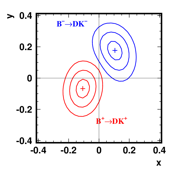
Figure 5 shows the projections of the three-dimensional confidence regions onto the $(r,\phi_{3})$ and $(\phi_{3},\delta)$ planes for the $B^{\pm}\to DK^{\pm}$ and $B^{\pm}\to D^{*}K^{\pm}$ modes. In the results for the $B^{\pm}\to D^{*}K^{\pm}$ mode, we combine both $D^{*}\to D\pi^{0}$ and $D^{*}\to D\gamma$ final states, taking into account the relative strong phase of $180{}^{\circ}$ between them by swapping the sign of the $x,y$ parameters for the $D^{*}\to D\gamma$ mode. We show the 20%, 74% and 97% confidence level regions, which correspond to one, two, and three standard deviations for a three-dimensional Gaussian distribution. The values of the parameters $r$, $\phi_{3}$ and $\delta$ obtained for the $B^{\pm}\to DK^{\pm}$ and $B^{\pm}\to D^{*}K^{\pm}$ modes separately are given in Table 3. The values of $\phi_{3}$ in these modes agree within the statistical errors. In general, $r$ and $\delta$ may differ: our results for $r$ are similar for the two modes, while the $\delta$ values are distinct.

Note that our statistical procedure gives three-dimensional confidence level regions. The coverage for the set of three parameters $(r,\phi_{3},\delta)$ is exact. One-dimensional intervals are obtained by projecting the three-dimensional regions onto each of the parameter axes: exact coverage for this procedure is ensured only in the case of Gaussian errors. In our case, Gaussian behavior of the errors is reached when $\sigma(r)\ll r$, and undercoverage (effectively, underestimation of statistical errors) occurs if $\sigma(r)\sim r$. The amount of undercoverage depends on the true value, $\bar{r}$: errors are underestimated by a factor ranging from 1.4 for $\bar{r}=0$, to 1.03 for $\bar{r}$ equal to the measured value.

Experimental systematic errors come from uncertainty in the knowledge of the distributions used in the fit (i.e. Dalitz plot distributions of the background components, and the $(M_{\rm bc},\Delta E)$ and $(\cos\theta_{\rm thr},\mathcal{F})$ distributions of the backgrounds and signal), fractions of different background components, and the distribution of the efficiency across the Dalitz plot. Uncertainties in background shapes are estimated by using alternative distributions in the fit (extracted from experimental data where possible). Uncertainties in the background fractions are obtained by varying each fraction within its error. Possible correlations in the distributions for background components that are not described by the formula (3) are estimated by using independent background distributions in the bins of $M_{\rm bc}$, $\Delta E$, $\cos\theta_{\rm thr}$ and $\mathcal{F}$ variables.

In case of $B^{\pm}\to D^{*}K^{\pm}$, $D^{*}\to D\gamma$ decay, an additional uncertainty arises from the significant cross-feed from the $B^{\pm}\to D^{*}K^{\pm}$, $D^{*}\to D\pi^{0}$ mode. The baseline $D^{*}\to D\gamma$ fit uses $x,y$ values obtained from the $B^{\pm}\to D^{*}K^{\pm}$, $D^{*}\to D\pi^{0}$ fit for modelling the $D^{*}\to D\pi^{0}$ cross-feed; to estimate the systematic uncertainty, we vary $x,y$ within their errors and also take $x=y=0$. As an additional check, we apply a $D^{*}\to D\pi^{0}$ veto to the $B^{\pm}\to D^{*}K^{\pm}$, $D^{*}\to D\gamma$ sample: the results of this fit are consistent with the baseline results within statistical errors.

References

- [1] M. Kobayashi and T. Maskawa, Prog. Theor. Phys. 49, 652 (1973); N. Cabibbo, Phys. Rev. Lett. 10, 531 (1963).
- [2] M. Gronau and D. London, Phys. Lett. B253, 483 (1991); M. Gronau and D. Wyler, Phys. Lett. B265, 172 (1991).
- [3] I. Dunietz, Phys. Lett. B270, 75 (1991).
- [4] D. Atwood, G. Eilam, M. Gronau and A. Soni, Phys. Lett. B341, 372 (1995).
- [5] D. Atwood, I. Dunietz and A. Soni, Phys. Rev. Lett. 78, 3257 (1997); D. Atwood, I. Dunietz and A. Soni, Phys. Rev. D 63, 036005 (2001).
- [6] I. I. Bigi and A. I. Sanda, Phys. Lett. B211, 213 (1988); A. B. Carter and A. I. Sanda, Phys. Rev. Lett 45, 952 (1980).
- [7] A. Giri, Yu. Grossman, A. Soffer, J. Zupan, Phys. Rev. D 68, 054018 (2003).
- [8] A. Bondar. Proceedings of BINP Special Analysis Meeting on Dalitz Analysis, 24-26 Sep. 2002, unpublished.
- [9] L. Wolfenstein, Phys. Rev. Lett. 51, 1945 (1983).
- [10] A. J. Schwartz (for HFAG charm group), arXiv:0911.1464 [hep-ex].
- [11] Y. Grossman, A. Soffer, J. Zupan, Phys. Rev. D 72, 031501 (2005).
- [12] Belle Collaboration, A. Poluektov et al., Phys. Rev. D 73, 112009 (2006).
- [13] Belle Collaboration, K. Abe et al., arXiv:hep-ex/0308043.
- [14] Belle Collaboration, A. Poluektov et al., Phys. Rev. D 70, 072003 (2004).
- [15] BaBar Collaboration, B. Aubert et al., Phys. Rev. Lett. 95, 121802 (2005).
- [16] BaBar Collaboration, B. Aubert et al., Phys. Rev. D 78, 034023 (2008).
- [17] BaBar Collaboration, B. Aubert et al., Phys. Rev. Lett. 99, 251801 (2007).
- [18] Belle Collaboration, A. Abashian et al., Nucl. Instr. and Meth. A 479, 117 (2002).
- [19] Y. Ushiroda (Belle SVD2 Group), Nucl. Instr. and Meth. A 511, 6 (2003).
- [20] A. Bondar and T. Gershon, Phys. Rev. D 70, 091503 (2004).
- [21] CLEO Collaboration, D. M. Asner et al., Phys. Rev. D 53, 1039 (1996).
- [22] Particle Data Group, C. Amsler et al., Phys. Lett. B 667, 1 (2008).
- [23] V. V. Anisovich and A. V. Sarantsev, Eur. Phys. J. A 16, 229 (2003).
- [24] CLEO Collaboration, S. Kopp et al., Phys. Rev. D 63, 092001 (2001).
- [25] CLEO Collaboration, H. Muramatsu et al., Phys. Rev. Lett. 89, 251802 (2002), Erratum-ibid: 90, 059901 (2003).
- [26] E791 Collaboration, E. M. Aitala et al., Phys. Rev. Lett. 86, 770 (2001).
- [27] ARGUS Collaboration, H. Albrecht et al., Phys. Lett. B 241, 278 (1990).
- [28] CLEO Collaboration, R.A. Briere et al., Phys. Rev. D 80, 032002 (2009).
- [29] A. Bondar, A. Poluektov, Eur. Phys. J. C 47, 347 (2006).
- [30] A. Bondar, A. Poluektov, Eur. Phys. J. C 55, 51 (2008).