A method for dense packing discovery
Abstract
The problem of packing a system of particles as densely as possible is foundational in the field of discrete geometry and is a powerful model in the material and biological sciences. As packing problems retreat from the reach of solution by analytic constructions, the importance of an efficient numerical method for conducting de novo (from-scratch) searches for dense packings becomes crucial. In this paper, we use the divide and concur framework to develop a general search method for the solution of periodic constraint problems, and we apply it to the discovery of dense periodic packings. An important feature of the method is the integration of the unit cell parameters with the other packing variables in the definition of the configuration space. The method we present led to improvements in the densest-known tetrahedron packing which are reported in Ref. [1]. Here, we use the method to reproduce the densest known lattice sphere packings and the best known lattice kissing arrangements in up to 14 and 11 dimensions respectively (the first such numerical evidence for their optimality in some of these dimensions). For non-spherical particles, we report a new dense packing of regular four-dimensional simplices with density and with a similar structure to the densest known tetrahedron packing.
pacs
61.50.Ah, 45.70.-n, 02.70.-cI Introduction
The dense packing behavior of a general solid body (particle) in a Euclidean space is a problem of interest in mathematics, physics, and many other fields. A packing is a collection of particles in the Euclidean space , wherein no two particles overlap (i.e., the intersection of any two particles has an empty interior) and the packing fraction or density is then the volume fraction of space covered by the particles. Of particular interest are packings of a given particle (wherein all particles are congruent), and the problem of interest is to determine the maximum possible density among all packings of a given particle. A packing that realizes this maximum can be thought of as the equilibrium state of the system of classical hard particles in the limit of infinite pressure or zero temperature.
The general problem of packing congruent particles was posed as a part of the eighteenth of David Hilbert’s famous Mathematische Probleme:
How can one arrange most densely in space an infinite number of equal solids of a given form, e.g., spheres with given radii or regular tetrahedra with given edges (or in prescribed position), that is, how can one so fit them together that the ratio of the filled to the unfilled space may be as large as possible? [2]
This part of the problem has been taken over the years as the resolution of the Kepler conjecture about the densest packing of spheres in three dimensions [3], and has therefore been considered resolved since the latter was proved by Hales [4]. However, Hilbert’s statement of the problem does not single out the sphere, and actually mentions the regular tetrahedron as another particle of interest. Recent work diverging from the focus on spherical particles has spotlighted ellipsoids [5], regular and semi-regular polyhedra [6, 7] (and the regular tetrahedron in particular [8, 9, 1, 10, 11]), and superballs [12]. Few bounds are known for the maximum packing fraction of general convex particles. Kuperberg and Kuperberg have shown that for any convex particle in two dimensions, [13]. Torquato et al. used the known maximal packing density of spheres to derive an upper bound on the packing density of any solid, but this bound is trivial (i.e., , where ) for many solids [6]. Ulam has conjectured that in three dimensions, the sphere achieves the lowest maximum packing fraction, , among all convex particles [14].
In the quest for dense packings of various particles, analytic and numerical investigations have both played important roles. The former have been very successful in the study of the dense packing of spheres, where analytic constructions based on groups, codes, and laminated lattices have produced the densest-known sphere packings and lattice sphere packings in many dimensions [15]. However, the analytic approach to the construction of dense packings relies on the imagination of the constructor, and for a variety of other problems the densest packings have evaded the creativity of analytic investigators and were only uncovered in computational investigations. While complete (i.e., exhaustive) algorithms exist for some problems (such as the algorithm in Ref. [16], which gave new best known results for the lattice covering and covering-packing problems in some dimensions), they do not exist or have runtimes that are too long for other problems. In those cases, incomplete search algorithms become necessary.
One example of a dense packing that has only been uncovered by a de novo numerical search is the currently densest-known packing of tetrahedra, whose structure was first hinted at by a numerical search using the method described in this paper [1]. The structure was later optimized by Torquato and Jiao [10] and by Chen et al. [11]. Results of subsequent Monte Carlo simulations have reproduced this structure and suggest it is the densest packing of regular tetrahedra at least with a small number () of tetrahedra in the unit cell [10, 11]. Another de novo search with Monte Carlo dynamics has uncovered a packing based on a quasicrystal approximant reminiscent of the Frank-Kasper -phase with a slightly lower density [9]. As these two structures were overlooked by previous analytical investigations [8, 17], it is quite likely that without the results of de novo searches, they would have remained unimagined and undiscovered.
In the best case, such searches would produce the optimal packing possible subject to the built-in restrictions (such as number of particles in the unit cell or unit cell shape). However, in problems exhibiting a large degree of frustration, the presence of many local optima that are separated from each other by high barriers complicates the task of finding the optimal packing. The tendency of simulations to get stuck in the local optima of such a rugged optimization landscape, especially when these local optima proliferate as more particles are simulated, has been held responsible for suboptimal results in searches [6, 7]. One technique which has been observed to relieve dynamical stagnation in Monte Carlo simulations at high pressures has been to allow slightly unphysical moves, such as allowing particles to temporarily overlap [9].
We propose a novel search method as an alternative to Monte Carlo simulations, with a number of features that directly address these observations. The method is based on the dynamics of the difference map, a constraint-satisfaction iterative search algorithm, and on the divide and concur constraint framework (we abbreviate this combination , where the minus sign stands for the difference map) [18, 19, 20]. It adapts the approach to the case of periodic problems and we shall call it periodic divide and concur (PDC). The difference map is designed to avoid being trapped in local optima and has been demonstrated in multiple applications to find solutions of highly non-convex problems, including finite packing problems with large numbers of particles, from random starting configurations [18, 19, 20]. The search proceeds through a non-physical configuration space, cutting through the conventional physical optimization landscape. Still, it is to be expected that the exponential growth in the number of local optima in the configuration space, which the search will still have to traverse, will nevertheless lead to suboptimal results when many independent particles are included in the search. Therefore, as discussed below, it is crucial for the unit cell variables to be aggressively optimized so that the number of particles to be simulated can be reduced. The incorporation of the unit cell variables directly into the basic dynamics of the search achieves this goal.
Numerical searches are restricted to finite-dimensional configuration spaces, and therefore have been largely limited to investigating periodic packings, packings which are preserved under translations by a lattice . In a general periodic packing, the particles are partitioned into orbits of the lattice , and when the packing is called a lattice packing. In physics, any periodic arrangement is usually referred to as a lattice and the special case of is known as a Bravais lattice. In general, the maximum density need not be realizable by a periodic packing, but arbitrarily close densities are realizable with periodic packings of arbitrarily large . Similarly, arbitrarily accurate approximations of any packing can be obtained using a sufficiently large cubic or orthorhombic unit cell. However, due to the rapid increase in computational complexity and the proliferation of local optima as the number of independent particles rises, it is often preferable to include fewer particles but allow for a variable unit cell shape. We focus then on searching for packings with a small number of particles in the unit cell.
To our knowledge, variable unit cells have only been introduced recently to searches for dense packings, for instance with the adaptive shrinking cell scheme in Refs. [5, 7] and with the use of Parrinello-Rahman dynamics in the space of lattices in Ref. [21]. The increased particle population associated with restricting unit cell variability can sometimes be tolerated in two and three dimensions, but in high dimensions the number of particles that must be simulated grows exponentially due to the curse of dimensionality and this approach becomes impractical. The constraint-satisfaction formulation of the periodic packing problem used in PDC features a variable unit cell and naturally treats the positions of particles in the unit cell and the unit cell parameters on the same footing. This new approach allows us to successfully look for dense sphere packings in dimensions as high as 14, further than probed by any previously reported unbiased numerical exploration of periodic packings.
Besides the density of a packing, another attribute of interest is the coordination number, that is, the number of nearest neighbors of particles in the packing. In the case of spherical particles, this amounts to the number of spheres in contact with a given sphere, known as the kissing number [15]. Searching for high-coordination number arrangements around a single sphere has been accomplished previously with the method [19]. Here we apply PDC to search for space-filling periodic arrangements of high coordination number, and particularly lattice arrangements.
An efficient de novo numerical search method can provide critical utility in the field of packing. In addition to the ability of a de novo search to provide confidence in a putative, but not proven, optimal result, a de novo search has often been responsible for surprising new results: two recent examples in which unexpected (as it turns out, quasiperiodic) packings were found as the results of de novo searches are in the problem of tetrahedron packing [9] and in the ten-dimensional kissing number problem [22]. It is with these motivations that we introduce the PDC method in this paper. In Section II we introduce the scheme by presenting a simple example which serves to motivate the constructions in the subsequent sections. In Section III we formulate the problems tackled in this paper — sphere packing, the lattice kissing number, and polytope packing — in terms of constraint satisfaction. In Section IV we describe in detail aspects of our implementation of the PDC search, including efficient computation of projections to the constraints of Section III. In Section V we present some results of PDC for the problems discussed, including a newly discovered packing of regular four-dimensional simplices. In Section VI we present concluding remarks.
II Motivation
II.1 The scheme
The key step in applying the approach to packing problems is to recast the problem as a problem of constraint satisfaction. Particularly, we must express it as the problem of finding a configuration in a Euclidean configuration space (), which satisfies two constraints. We identify a constraint with the subset of configurations satisfying the constraint. A projection of a configuration to a constraint is the operation of finding a configuration that minimizes the distance . Each of the two constraints (), must be simple enough that the operation of projecting an arbitrary configuration to it can be computed efficiently. The iterative map used in exploring the configuration space takes advantage of the formulation of the problem in terms of two simple constraints, as outlined in section II.2. In this section we present the application of the scheme to finite sphere packing problems, which has been developed and implemented in Ref. [19], as an introduction to the main ideas of the scheme.
The defining constraint of packing problems is the constraint that no particles in the packing overlap, which we call the exclusion constraint. As a simple illustration of this constraint, consider the exclusion of a pair of unit-radius disks in . In this case, the configuration space is parameterized by the positions of the centers of the two disks:
| (1) |
The exclusion constraint is then
| (2) |
This constraint adheres to the simplicity criterion of having an efficient method to compute a projection to it. Specifically, the projection is given by
| (3) |
where,
| (4) | ||||
| (5) |
as illustrated in Figure 1.

A more complicated case arises when three or more disks are considered. In this case, the exclusion constraint,
is not a simple constraint according to the criterion above. Alternatively, we could replace by many pairwise exclusion constraints
| (6) |
The pairwise constraints are all individually simple. However, as noted above, we are limited to problems described by only two simple constraints.
Divide and concur provides a general procedure for reducing the number of simple constraints to two, at the expense of enlarging the configuration space. This reduction is achieved by parameterizing the configuration space with more variables than are necessary to fully specify a configuration. In the example at hand, the new configuration space is
| (7) |
where we call all the variables for a particular index the replicas of the original variable . Every configuration can be identified with a configuration , wherein for all , through a simple linear map . Enough redundant variables have been introduced to the configuration space so that each pairwise exclusion constraint can now be written in terms of a private set of variables, disjoint from the private variables of other constraints:
| (8) |
The intersection, , of all of the pairwise exclusion constraints, which we will call the “divide” constraint, is now also simple, since the projection can be performed independently on each set of private variables (Figure 1).
The map from the original configuration space (the physical configuration space) to the new one (the formal configuration space) is not surjective, and so a general point in the formal configuration space does not correspond to a valid physical configuration. The “concur” constraint is given by the range of , the subset of that does correspond to valid configurations. That is, the constraint requires redundant specifications of an original variable to concur in regard to its value. Since is linear, is also a simple constraint.
Another constraint that must usually be addressed in packing problems with a finite number of particles is the confinement constraint. In most cases the particles, or their centers, are confined to lie in some subset of space, where can be either some region of finite volume, or a compact manifold (as in the case of spherical codes). As a subset of the original configuration space, the confinement constraint is written as
| (9) |
We can incorporate this constraint into the “concur” constraint, , by modifying it to be the image instead of the entire range of . In our example, this would give the constraint
| (10) |
Since is linear, the projection to can be decomposed into a projection to followed by a projection to . The first step is performed by taking the average position of all the replicas of each disk. The second step is performed by projecting this average position to (see Figure 1). In general, this two-step projection method is valid for handling the constraints in the physical configuration space that are simple at the outset and do not require the introduction of new variables.
The result of the above construction is that a configuration in satisfies the “divide” and “concur” constraints simultaneously if and only if it corresponds to a configuration in which satisfies all the exclusion constraints and the confinement constraint; that is, it corresponds to a solution of the packing problem under consideration.
In the following sections we modify the above simple construction so as to generalize the method in two major ways. The first generalization is to packings of infinite regions, instead of only finite ones. Specifically, we allow for periodic packings with an arbitrary unit cell. This is achieved by generalizing the idea of replicas of particles to include also their periodic images. When the unit cell vectors are included in the original set of parameters, the map from the original parameter space to the space of replica configurations is still linear, though a little more elaborate. Additionally, the confinement constraint of finite packings is replaced in the case of periodic packings by a constraint on the unit cell volume, ensuring a specified density.
The second generalization is to packings of non-spherical particles, specifically convex polytopes. This is achieved by representing each particle not only by the position of its centroid, but by the positions of all its vertices. A new constraint, the rigidity constraint, is added to ensure that the particle is not deformed in the solution. Despite the mathematical complications that arise from these two generalizations, the conceptual framework is identical to the above example, and the constructions in the following sections will draw attention to the analogy with the construction presented above.
II.2 The difference map
Given a problem formulated as the task of finding a configuration , simultaneously satisfying the constraints , we wish to use the availability of efficient methods for computing the projections and to the constraints in order to set up an iterated map to search through the configuration space for a solution. Naive schemes, such as the alternating projections map , suffer from the problem of stagnation at near solutions (local minima of the distance between the two constraints). The difference map, a slightly more sophisticated scheme, is designed to provide efficient search dynamics while avoiding the traps of local minima [18].
The difference map (DM) can be written in terms of the projections and and one parameter :
| (11) |
| (12) |
where
In this paper we use only . A difference map search proceeds by starting from a random initial configuration and iteratively applying the difference map: [18]. When the map reaches a fixed point , a solution is obtained by
| (13) |
Notice that the ability to obtain a solution from any fixed point of the map, due to the cancelation of the two bracketed terms in (12), relies on the definition of the problem in terms of only two simple constraints. For a given iterate , the terms and provide two estimates of the solution, each satisfying one of the two constraints. We call these respectively the - and -estimates of the solution at the th iteration. The distance between the two estimates is the error and the search terminates when the error converges to zero.
To summarize, a simple difference map solver for continuous constraints would consist of the following simple steps:
- 1.
Initialize the iterate to a random configuration.
- 2.
Compute the two estimates of the solution and .
- 3.
Compute the error . If it is below a predefined convergence threshold, the search terminates, and the solution is given by .
- 4.
Advance the iterate . Start the next iteration at Step 2.
III Constraints
III.1 Periodic sphere packing and kissing
A periodic packing of equal-sized spheres (radius ) in dimensions can be generated by the action of a lattice on a set of primitive spheres. Let be the set of centers of the primitive spheres. We define a generating matrix of the packing as a matrix whose first rows are a set of generators of and whose remaining rows are the vectors in the set . Combining these quite different sets of configuration variables into a single matrix serves to remind us that at the highest level of our search algorithm both sets are treated in a uniform manner by the projection operators. The detailed constraints, of course, distinguish among the two parts of , which we denote (lattice generators) and (primitive sphere centers). The set of all the centers of spheres in the packing is then the Minkowski sum
| (14) | ||||
where is the set of coordinate-permutations of the -dimensional vector . The space of generating matrices takes the role of the physical configuration space .
A matrix generates a valid packing if the centers of any two sphere of the packing, and , are separated at least by a distance of when . Each choice of and generates a constraint on the matrix
| (15) |
which we call an exclusion constraint. Note that there are infinitely many independent exclusion constraints (constraints with are not independent). However, for any non-degenerate matrix only finitely many independent exclusion constraints are violated or are even remotely close to being violated. In practice, only those constraints need be tested in our computations. We call those constraints the relevant exclusion constraints (let there be of them), and we define a matrix whose rows and are the vectors and related to the th relevant exclusion constraint. We discuss below how the relevant constraints are identified.
The linear map is a map from the physical configuration space to a larger-dimensional space, , which we use as the formal configuration space. As before, since the map is not surjective, only a subset (a linear subspace, in fact) of formal configurations have a corresponding generating matrix in the physical configuration space. The choice of constraints below will guarantee that solutions belong to this subset. The size of the configuration space grows as the number of relevant independent exclusion constraints, which is the number of independent near neighbor pairs for which overlap needs to be actively avoided. Notice that each relevant exclusion constraint can now be written in terms of a private set of variables. Specifically, each row of the matrix corresponds to the position of one particle, and the th relevant exclusion constraint is given by
| (16) |
The intersection of all the relevant exclusion constraints forms our “divide” constraint,
| (17) |
Each set of private variables associated with one exclusion constraint is composed of the coordinates of replicas of two particles, and we call these two replicas a replica pair.
As mentioned in Section II.1, the confinement constraint of finite packing problems is replaced in the case of periodic packings with a constraint on the density of the packing. The density of a packing generated by a matrix is given by the density of the unit cell, whose volume is and which contains particles of volume :
| (18) |
Therefore, if we wish to find a packing of density , the density constraint on the generating matrix will be
| (19) |
where .
As in the example of Section II.1, since the map is not surjective, a general element of the formal configuration space does not correspond to a well-defined physical configuration. We therefore impose a constraint that requires to lie in the range of . In the context of the PDC construction we call this the lattice constraint because it requires different periodic images of a primitive particle to lie on the points of a lattice, and requires that lattice to be the same for all primitive particles (up to translation). Again, as in Section II.1, we combine the lattice constraint with the density constraint to form the “concur” constraint:
| (20) | ||||
With these definitions of the constraint sets, if and only if generates a periodic packing of density . The action of the projections and to the two constraints is illustrated in Figure 2 and Sections IV.1 and IV.2 discuss how the projections are computed efficiently.
The basic operations of the search — projections — depend directly on the metric defined on the formal configuration space. Therefore, the choice of metric affects both the complexity of implementing the projection and the search dynamics. The simplest choice for the metric is the distance induced from the Frobenius (Euclidean) norm
| (21) |
This choice of metric amounts to giving all replicas of a particle equal weight in influencing its consensus position in the “concur” projection. We can use a slightly different Euclidean metric, given by
| (22) |
where is a diagonal matrix whose diagonal elements are the metric weights of different replicas. Performance is greatly enhanced by adjusting the metric weights throughout the search to afford greater weight to replica pairs that continually violate their constraints and smaller weight to replica pairs that are in low risk of violating their constraints [19]. Note that removing a constraint from the list of relevant constraints (i.e., removing the corresponding pair of rows from and ) is equivalent to setting the metric weight of its replicas to zero. Therefore, in the course of the search we not only adjust the weights of replica pairs, but also add and remove replica pairs. The details of how these changes are applied systematically are given in Section IV.3.
This constraint formulation of the periodic sphere packing problem (finding a periodic packing with density ) can be straightforwardly modified to describe instead the periodic kissing number problem (finding a periodic packing with average coordination number ). First, the “divide” constraint is modified so that each replica pair must still be separated by a distance of at least , but at least replica pairs must be separated by a distance of exactly . Second, the condition on the volume of the unit cell is dropped from the “concur” constraint. Projections to these modified constraints are also given in Section IV.

III.2 Convex polytope packing
The symmetry of the spherical particle allows its configuration to be described solely by the position of its center. In the case of a general convex particle, the variables of the configuration space need to include information also about the orientation of the particle. One possible description of the particle assigns variables separately to the position of its centroid and to the description of the rotation about the centroid (e.g., a rotation matrix or a quaternion). In this paper, however, we find it more convenient to describe convex polytopes by reference to the positions of their vertices. Therefore, a polytope with vertices is represented by a vertex matrix and is given by the convex hull of these vertices. Although the configuration of a single particle is no longer represented by a single vector but by a matrix composed of vectors, it is convenient to treat these matrices as vectors, which we typeset as bold-face upper-case Latin letters (e.g., for the vertex matrix of the polytope ), and to construct matrices whose rows are such vectors. A translation by of a polytope is given by , where is a column vector of unit elements and is the translation matrix corresponding to the translation vector . Similarly, a rotation is given by , where is a orthogonal matrix.
A periodic packing is again generated by the action of a lattice on a set of primitive polytopes whose vertex matrices form the set . The set of all vertex matrices of polytopes in the packing is the Minkowski sum
| (23) | ||||
where is a generating matrix of the packing, whose first rows (comprising ) are translation matrices generating , and whose remaining rows (comprising ) are the vertex matrices of the set . The space of generating matrices is the physical configuration space.
Each exclusion constraint between two particles of the packing requires the convex hulls and not to overlap for any . To construct the formal configuration space we again form one replica pair for the particles involved in each relevant exclusion constraint, which gives . The map from physical configurations to formal configurations is given by the matrix whose rows and are the vectors and related to the th relevant exclusion constraint. The “divide” constraint is given by the intersection of all the relevant exclusion constraints, each expressed in terms of its private replica pair:
| (24) | ||||
In addition to the lattice constraint and the density constraints, which combine in Section III.1 to form the “concur” constraint, in the case at hand we must include a third constraint, the rigidity constraint. The primitive particles of a packing generated by a general matrix are only constrained in their number of vertices, not in the arrangement of those vertices. However, we are interested only in packing where all the particles are congruent with a given shape, and so we impose the constraint on that the vertices of its primitive particles are obtained from the vertices of the given particle by a rigid motion:
| (25) | ||||
| for all rows of |
where is the vertex matrix of the given particle. The “concur” constraint is given by combining the density and rigidity constraints on the generating matrix with the lattice constraint. The result of constructing the “divide” and “concur” constraints is that a formal configuration satisfies both of them if and only if it corresponds to a generating matrix in the physical configuration space which yields a packing of the given particle with the desired density. Table 1 summarizes the constraints for the three problems discussed and Section IV describes in detail the projections to these constraints.
| “divide” constraint | “concur” constraint | |
| sphere | for | |
| packing | all replica pairs | |
| kissing | for | |
| number | all replica pairs and | |
| for pairs | ||
| polytope | convex hulls of | |
| packing | and non-overlap- | |
| ping for all replica | and | |
| pairs |
IV Implementation
IV.1 “Divide” projections
IV.1.1 Sphere packing and kissing
In order to implement an iterated difference map search, whose iterations are given by (12), we must implement efficient projections to the “divide” and “concur” constraints. These implementations are the subject of Sections IV.1 and IV.2. In the course of the search, considerations of efficiency require certain changes to the formal configuration space – specifically adding and removing replica pairs, changing metric weights, and lattice reduction. In section IV.3 we discuss when and how these changes are applied.
In the case of sphere packing, the “divide” constraint simply requires that the centers of the two spheres comprising each replica pair be a certain distance apart. This is obtained by applying equation (3) to each replica pair. Note that the “divide” projection acts independently on each replica pair, and since the metric weight of all variables specifying one replica pair are equal, the metric weights have no influence on this projection. The action of this projection is illustrated in Figure 2. For the kissing number problem, the first case of (3) is also used if the replica pair is one of the closest replica pairs.
IV.1.2 Convex polytope packing

Although identifying and resolving overlaps between two spheres is straightforward, the same task is more challenging in the case of other convex objects, where more degrees of freedom come into play. The literature on the topic of detecting overlaps (collisions) between polyhedral solids is extensive (driven in part by applications in computer graphics), and many efficient techniques exist for checking whether two convex polyhedra, and , overlap (see e.g., [23, 24]). In our case, as we are interested in computing the projection to the exclusion constraint, we also need to determine the distance-minimizing resolution of the overlap. That is, we must find the smallest displacement of the vertices such that the new polyhedra do not overlap. As far as we have been able to determine, there is not an established, efficient computational method developed for this specific problem. The method we provide here is efficient enough for the purpose of packing polyhedra with a small number of vertices, but the computation time required grows exponentially with the number of vertices. A more efficient resolution method for particles with more vertices and for smooth particles is currently in development.
The method relies on the separating plane theorem: the convex hulls of two sets of vertices in do not overlap if and only if there is a -dimensional plane that separates the two sets, so that each is contained in a different half-space. The theorem can be made even stronger by specifying that the separating plane can always be chosen to contain vertices from the given sets, including at least one from each. Therefore, one can check whether two polytopes overlap by checking whether they are separated by any of the planes defined by any such subset of vertices (Figure 3a–b). If the polytopes are non-overlapping, the resolution leaves the vertices unchanged.
If the polytopes overlap, we must find the smallest displacement of their vertices that resolves the overlap. In the resolved configuration there is a separating plane, , that separates the two sets of vertices. As a consequence of distance minimization, the only vertices moved in the course of the resolution are the vertices which lie on in the resolved configuration. Let and be the pre- and post-resolution positions, respectively, of those vertices that are displaced during the resolution. Therefore, is the set of points in closest to the points of :
| (26) |
The squared norm of the resolution displacement is
| (27) |
For any set of points there is at least one plane that minimizes the sum of squared distances
| (28) |
We call such a plane a least-squares plane of . The separating plane of the resolved configuration is always a least-squares plane of . If this were not the case, a small tilting of the separating plane towards such a least-squares plane (with a corresponding movement of the points in ) would result in a resolution by a smaller displacement. In order to resolve an overlap between polytopes and , we therefore have to solve a discrete problem: among all subsets of with a least-squares plane separating the remaining vertices from , find the one with the minimal sum of squared distances (28). This is the set (Figure 3c–f).
The least-squares plane of a set is determined by minimizing the sum of squared distances (28). Note that for a fixed normal direction , the value of that minimizes the sum is , where is the centroid of . Therefore, we wish to minimize
| (29) |
the minimum of which is equal to the smallest eigenvalue of the symmetric matrix . The minimum is realized when is the corresponding eigenvector. Degenerate cases with equal lowest eigenvalues occur, but they do not pose a problem: whenever an optimal separating plane occurs as a degenerate least-squares plane of some set , its degeneracy implies that there is a least-squares plane of which also includes an extra vertex; this plane will be equally optimal and will occur as a less degenerate least-squares plane of a superset . Therefore, the optimal least-squares plane always occurs as a non-degenerate least-squares plane of a set .
To summarize, the overlap detection and resolution algorithm consists of three steps (illustrated in Figure 3a–f):
- 1.
Consider all subsets of size with at least one point from each polytope. Let be a plane that includes . For each let
(30) (31) (32) and let
(33) provides a measure for the interpenetration of the two polytopes. If , then a separating plane exists, the input polytopes do not overlap, and the algorithm ends here by returning the original vertex positions and . If , the polytopes overlap and the algorithm continues to Step 2.
- 2.
Consider all subsets of size with at least one point from each polytope. Let be a least-squares plane of . If the plane separates the vertex sets with the points of removed — and — let be the sum of squared-distances from to the plane. Otherwise, let . Among the subsets considered, let be the subset that minimizes and be its associated least-squares plane. As if contains all vertices, the minimum is always finite. Continue to Step 3.
- 3.
The sets of vertices returned are given by and , wherein is given by
(34) where is the corresponding original vertex position.
The projection to the “divide” constraint (24), of an input matrix comprised of pairs of vertex matrices and , is then achieved by applying the above algorithm independently to all pairs.
IV.2 “Concur” projections
IV.2.1 Lattice constraint
All the “concur” constraint sets described in this paper are of the form
| (35) |
where is constant, and is variable, but must satisfy a constraint . The projection then is given by
| (36) |
where realizes the minimum over of the distance
| (37) |
Absent any constraints on (as for example in the “concur” constraint for the kissing number problem, where ), the solution would be given by
| (38) |
This can easily be seen by writing , which gives
| (39) |
where and the constant term does not depend on . The second term is non-negative, and when is unconstrained, (39) is minimized by letting . Additionally, we have just reduced the constrained case to the problem of finding that minimizes the cost function
| (40) |
This projection strategy parallels the two-step strategy used in Section II.1. First, the formal configuration is projected to the range of the physical configuration space, giving . Then, the projection of to the additional constraint is performed in the physical configuration space using the metric induced on its image in the formal configuration space. Below, we solve the second step of this projection problem for various constraints .
IV.2.2 Density constraint
In the “concur” constraint for the sphere packing problem, the only constraint on the generating matrix is the density constraint. The set of generating matrices satisfying the density constraint is
| (41) |
where is the generating matrix of the lattice and is given by the first rows of . If , then the projection to the constraint (the choice of that minimizes the cost function (40)) is trivially . Otherwise, since is unconstrained, we can minimize (40) with respect to for a given . This yields , where are the block-elements of acting on to the left and on to the right. Thus, the cost function for is simply
| (42) |
where .
The projection becomes easier to analyze in terms of the matrix . The cost function then takes the form of the simple Frobenius distance
| (43) |
and the density constraint is still in the form
| (44) |
where . Since the absolute value of the determinant of is given by the product of its singular values, the solution to this minimization problem is given by a matrix with the same (right and left) singular vectors as the matrix , but different singular values. The cost function expressed in terms of the singular values and of, respectively, and takes the form
| (45) |
We numerically minimize this quadratic function subject to the density constraint (44). Through back substitution we then have the matrix that minimizes (37) and .
IV.2.3 Rigidity constraint
In the “concur” constraint for the polytope packing problem, an additional constraint on the generating matrix is that the primitive polytopes that make up are congruent with a given polytope. The generating matrix is then constrained to the set
| (46) |
where
To calculate the projection , the cost function (40) must be minimized over . However, since the off-diagonal block couples the lattice parameters to the primitive particle parameters , this minimization is complicated. Instead of exact minimization, we employ a two-step heuristic method, which results in an approximate projection.
In the first step, we calculate the matrix that minimizes the cost function, as in Section IV.2.2. Then, in the second step, we calculate the matrix by applying to each row of the smallest change so that it becomes a vertex matrix of a polytope congruent with the reference polytope. The second step is achieved by finding the rigid motion applied to the reference polytope which brings its vertices as close as possible to the vertices of as measured by the sum of squared distances (Figure 3g). The problem of finding the rigid motion that brings one given list of points closest to another given list, sometimes known as the problem of absolute orientation, occurs frequently in a variety of fields (e.g., in calculating RMSD between two conformations of a biomolecule) and several efficient methods for its solution have been developed (see [25, 26]).
The output of the approximate projection is then given by . As , the approximate projection gives a configuration in the constraint set, but might not give the closest one to the input configuration. We justify the use of the approximate projection by noting that it is an exact projection if the off-diagonal block is zero. A non-zero off-diagonal block is the result of correlations in the relevant exclusion constraint vectors between the coefficients of lattice translations and the coefficients of primitive particle vertex positions. We expect these coefficients to give uncorrelated contributions and to add up to small off-diagonal elements due to random cancellations. Indeed, we find that the off-diagonal block is small in comparison with the diagonal blocks, and we expect our heuristic to yield a good approximate projection.
IV.3 Formal configuration space maintenance
In our discussion of the choice of metric in Section III, we discussed the ideas of dynamically readjusting the metric (through the weights of the various replicas) and of removing and adding replicas (removing replicas is formally equivalent to setting their weight to zero). The latter is necessary for implementation reasons: there are infinitely many independent exclusion constraints (and therefore replicas), but we can only represent a finite number of replicas in our implementation. As the set of relevant constraints changes over the course of the search, we must remove and add replicas. Our criterion for which replicas to represent is based on the difference map’s current “concur” estimate: we include a replica pair for each pair of particles whose centroids in the “concur” estimate are closer than some cut-off distance. Using the generating matrix obtained in the “concur” projection we can easily find all such pairs using the method of Agrell et al. [27]. The cut-off distance is chosen so that at least all replicas that might be in risk of overlap are represented.
The problem of implementation is not the only reason we wish to limit the number of replicas we represent. A proliferation of unnecessary replicas has the adverse effect of attenuating the information obtained from the “concur” projection by diluting the influence of more critical replicas. We observe that such replica proliferation could result not only in a slower search, but also in an increased tendency to become trapped in local optima. Limiting the number of replicas is one way to avoid this effect, but we find it useful to further amplify the information from critical constraints by giving them greater weights [19]. We perform the weight adjustments adiabatically, that is, slowly over the course of many iterations, by updating the weights of each replica pair according to the rule
| (47) |
where is a function that assigns replicas weights based on their configuration in the “concur” estimate, and is a relaxation time for the replica weights in units of iterations.
In the sphere packing problem (in dimensions, with unit spheres), we choose the weight function to be
| (48) |
with . The dimensional dependence is chosen so that under the assumption of uniform density, the total weight from replicas over a certain distance follows a dimension-independent power law. In the polytope packing problem, we similarly use
| (49) |
with , where is the inradius of the polytope, is the centroid-centroid distance of the polytopes, and is the measure of the overlap between the polytopes defined in (33).
In addition to the maintenance of replicas, which is performed after every iteration of the difference map, we also periodically perform a lattice reduction using the LLL algorithm [28]. The lattice generated by is re-represented using the LLL-reduced generating matrix , where is a unimodular integer matrix. Additionally, all primitive particles whose centroids are outside of the unit cell given by are re-represented by their lattice-translate in that cell. In summary, the new packing generating matrix is given by
| (50) |
where gives the lattice translations to be applied to the primitive particles. Since the actual positions of the particles, as represented in the matrix , should be unchanged, the lattice reduction must also be applied to the nominally constant matrix ().
V Results
V.1 Sphere packing
Using the PDC scheme described in the previous sections we perform a de novo search for the densest lattice () sphere packings in dimensions —. The PDC search, starting from random initial configurations, was able to reproduce the densest packing lattices known for all cases, and the results of the search are summarized in Table 2. For dimensions — the lattices are known to be optimal, and for dimensions — these results are, to our knowledge, the first numerical evidence from a de novo search that the known lattices are optimal.
Note that the number of replicas is determined by the number of near neighbors of each sphere, which rises rapidly with the number of dimensions. This rise causes an increased computational storage cost per physical degree of freedom in a PDC search, compared to a constant storage cost per physical degree of freedom in a method involving a local search in the physical configuration space. However, this rise need not affect the scaling of CPU costs, since both search methods need necessarily check a comparable number of particle pairs for possible overlaps.
In dimensions there are known non-lattice packings with respectively that are denser than the densest known lattices [15]. In up to 11 dimensions, we searched for non-lattice packings with as many as primitive spheres, but the searches did not produce packings denser than the lattice packings. For a density target matching the lattice density, the searches reproduced the lattice packing, suggesting that the lattice packing in these dimensions is the optimal packing with a small number of spheres in the unit cell.
| success rate | ||||||
|---|---|---|---|---|---|---|
| 2 | ||||||
| 3 | ||||||
| 4 | ||||||
| 5 | ||||||
| 6 | ||||||
| 7 | ||||||
| 8 | ||||||
| 9 | ||||||
| 10 | ||||||
| 11 | ||||||
| 12 | ||||||
| 13 | ||||||
| 14 |
V.2 Kissing number
For the kissing number problem, PDC searches were able to reproduce the best known lattice kissing arrangements in dimensions —. In dimensions —, the result is known to be optimal, and for dimensions and , we are not aware of previous numerical evidence for their optimality. Table 3 summarizes the performance of our method.
| success rate | |||||
|---|---|---|---|---|---|
| 2 | |||||
| 3 | |||||
| 4 | |||||
| 5 | |||||
| 6 | |||||
| 7 | |||||
| 8 | |||||
| 9 | |||||
| 10 | |||||
| 11 |
V.3 Polytope packing
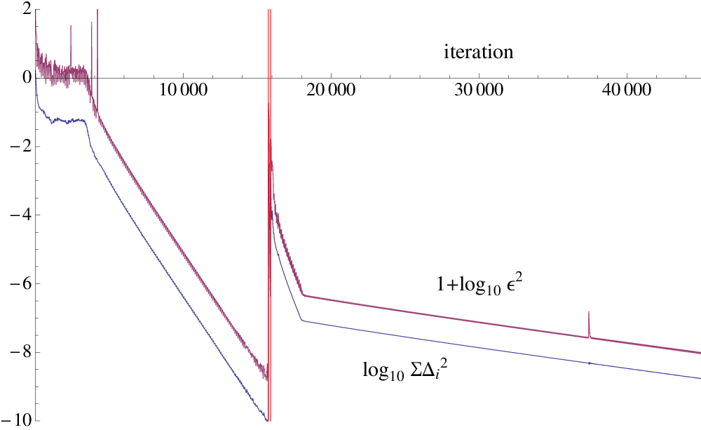
By inspection of a packing of regular tetrahedra yielded by our numerical search during early phases of its development, we were able to construct a new transitive, periodic () packing of tetrahedra with a higher density () than previously reported [1]. This packing takes the form of a double lattice of bipyramidal dimers (the union of two face-sharing tetrahedra). The packing has since been slightly improved to a closely related, but less symmetric packing with density [10, 11]. In its current form, our search method is able to reproduce this densest known packing reliably (fifteen out of a hundred runs converged within the iteration limit), and Figure 4 shows the results of a sample run converging to this packing.
For the problem of packing regular four-dimensional simplices (pentatopes) in four-dimensional Euclidean space, we report a new packing discovered by our search method (Figure 5). This packing, with density , is, to our knowledge, denser than any previously reported packing of regular pentatopes. Like the densest known tetrahedron packing, this packing also takes the form of a double lattice of dimers (a dimer here is the union of two cell-sharing pentatopes). This structure, composed of a repeating unit of two oppositely oriented dimers, repeatedly came up as the densest in de novo PDC searches with and pentatopes in the unit cell, whereas searches with intermediate values of yielded sparser packings. We subsequently refined the packing with a restricted search where the dimer was taken as the basic particle.
Note that the density reported is slightly lower than that of the densest known packing of four-dimensional spheres (). It remains to be determined whether this is the case because the optimal packing density of pentatopes is smaller than that of spheres or because the dimer double lattice is suboptimal. The vertex coordinates of the four primitive pentatopes and the generating matrix of the lattice are given in Table 4.


| primitive pentatopes | |
|---|---|
| where | |
| lattice | |
| where | |
VI Conclusion
In this article we report on the development of PDC, a novel, constraint-based method for discovering dense periodic packings through de novo numerical searches. We lay out the principles of the method and demonstrate its application for selected problems. In addition to the dense packing of regular tetrahedra reported in Ref. [1], we also discover a new dense packing of regular pentatopes using the PDC method. We also use the method to numerically recover the lattice sphere packings of highest known density and highest known kissing number in a range of dimensions, providing empirical evidence of their optimality.
In developing the PDC scheme, we adapt the framework to periodic systems. PDC retains the mindset of the traditional approach of Ref. [19], but generalizes its formalism in a few ways. We introduce an expanded configuration space parameterized by linear combinations of the original parameters, such that these new parameters over-determine the configuration. Therefore, by contrast with the traditional construction, where new parameters are, specifically, redundant copies of original parameters and concurrence is described by the equality of all copies of a given original parameter, here we allow concurrence to be described by a general linear relation. With this generalization, we can treat the periodic images of a particle as “replicas” of the particle, even as they are related by a lattice vector instead of being identical. Thus, the variables describing the periodic repetition of the configuration, namely the lattice vectors, are not imposed as constants or adjusted in dedicated steps. Instead, due to the projection formulation of the dynamics, the unit cell variables that minimize the change to the configuration are determined at each iteration. These variables are treated on the same footing as particle positions and orientations and are optimized as aggressively.
Additionally, we develop a displacement-minimizing overlap resolution algorithm for the convex hulls of two sets of points in . We use this algorithm to implement the projection to the exclusion constraint in the case of polytopal particles.
Unlike Monte Carlo simulations, which explore the physical optimization landscape using stochastic moves, a PDC search uses a deterministic map in an expanded, non-physical configuration space. As such, it is useful when interest lies more in discovering optimal configurations and less in discovering the physical pathways to such configurations. However, introducing non-physical dynamics has been observed to be important in overcoming dynamical stagnation [9]. The projection-based dynamics make PDC particularly well-suited in problems with hard constraints, such as hard particle packing, or with step potentials, which prohibit the use of gradient information.
While no direct comparison has been made between the performance of PDC and Monte Carlo searches in the case of periodic packing problems, difference map and methods in the case of other problems have been shown to perform better than or on a par with specialized and general-purpose methods [18, 19, 20, 29]. The generality of the PDC scheme and its demonstrated ability to discover dense packings in a variety of settings indicate its utility as a general method for conducting de novo numerical searches and as a possibly attractive alternative to conventional methods 11 1 An implementation of our algorithm is available upon request from the corresponding author..
Y. K. acknowledges N. Duane Loh for valuable discussions. This work was supported by grant NSF-DMR-0426568.
References
- [1] Y. Kallus, V. Elser, and S. Gravel, Discrete Compu. Geom. 44, 245 (2010).
- [2] D. Hilbert, Bull. Am. Math. Soc. 8, 437 (1902).
- [3] D. Rowe and J. Jeremy, The Hilbert Challenge (Oxford University Press, 2001).
- [4] T. C. Hales, Ann. Math. 162, 1065 (2005).
- [5] A. Donev, F. H. Stillinger, P. M. Chaikin, and S. Torquato, Phys. Rev. Lett. 92, 255506 (2004).
- [6] S. Torquato and Y. Jiao, Nature 460, 876 (2009a).
- [7] S. Torquato and Y. Jiao, Phys. Rev. E 80, 041104 (2009b).
- [8] E. R. Chen, Discrete Comput. Geom. 5, 214 (2008).
- [9] M. E. A. Haji-Akbari et al., Nature 462, 773 (2009).
- [10] S. Torquato and Y. Jiao, Phys. Rev. E 81, 041310 (2010).
- [11] E. R. Chen, M. Engel, and S. C. Glotzer, Discrete Compu. Geom. 44, 253 (2010).
- [12] Y. Jiao, F. H. Stillinger, and S. Torquato, Phys. Rev. E 79, 041309 (2009).
- [13] G. Kuperberg and W. Kuperberg, Discrete Compu. Geom. 5, 389 (1990).
- [14] M. Gardner, The Colossal Book of Mathematics: Classic Puzzles, Paradoxes, and Problems (Norton, New York, 2001).
- [15] J. H. Conway and N. J. A. Sloane, Sphere Packings, Lattices and Groups (Springer-Verlag, New York, 1998), 3rd ed.
- [16] A. Schürmann and F. Vallentin, Discrete Comput. Geom. 35, 73 (2006).
- [17] J. H. Conway and S. Torquato, Proc. Natl. Acad. Sci. USA 103, 10612 (2006).
- [18] V. Elser, I. Rankenburg, and P. Thibault, Proc. Natl. Acad. Sci. USA 104, 418 (2007).
- [19] S. Gravel and V. Elser, Phys. Rev. E 78, 036706 (2008).
- [20] S. Gravel, Ph.D. thesis, Cornell University, Ithaca, New York (2009).
- [21] H. Cohn, A. Kumar, and A. Schürmann, Phys. Rev. E (2010), accepted for publication.
- [22] V. Elser and S. Gravel, Discrete Comput. Geom. 43, 363 (2010).
- [23] G. van den Bergen, Proximity queries and penetration depth computation on 3d game objects (2001), game Developers Conference.
- [24] S. Cameron, in Proceedings of International Conference on Robotics and Automation (1997), p. 3112.
- [25] B. K. P. Horn, J. Opt. Soc. Am. A 4, 629 (1987).
- [26] B. K. P. Horn, H. M. Hilden, and S. Negahdaripour, J. Opt. Soc. Am. A 5, 1127 (1988).
- [27] E. Agrell et al., IEEE Trans. Inform. Theory 48, 2201 (2002).
- [28] A. K. Lenstra, H. W. Lenstra, and L. Lovász, Math. Ann. 261, 515 (1982).
- [29] V. Elser and I. Rankenburg, Phys. Rev. E 73, 026702 (2006).