Dynamical Symmetry Breaking With a Fourth Generation
Abstract
Adding a fourth generation to the Standard Model and assuming it to be valid up to some cutoff , we show that electroweak symmetry is broken by radiative corrections due to the fourth generation. The effects of the fourth generation are isolated using a Lagrangian with a genuine scalar without self-interactions at the classical level. For masses of the fourth generation consistent with electroweak precision data (including the CP asymmetries) we obtain a Higgs mass of the order of a few hundreds GeV and a cutoff around 1-2 TeV. We study the reliability of the perturbative treatment used to obtain these results taking into account the running of the Yukawa couplings of the fourth quark generation with the aid of the Renormalization Group (RG) equations, finding similar allowed values for the Higgs mass but a slightly lower cut-off due to the breaking of the perturbative regime. Such low cut-off means that the effects of new physics needed to describe electroweak interactions at energy above should be measurable at the LHC.We use the minimal supersymmetric extension of the standard model with four generations as an explicit example of models realizing the dynamical electroweak symmetry breaking by radiative corrections and containing new physics. Here, the cutoff is replaced by the masses of the squarks and electroweak symmetry breaking by radiative corrections requires the squark masses to be of the order of 1 TeV.
I Introduction.
Many experimental results on physics (see [1]) can be seen as hints of physics beyond the Standard Model (SM). Electroweak precision data also points to new physics scenarios [2]. In the LHC era, new physics related to the observability of the Higgs boson is worthy to study and the elucidation of the Higgs sector properties is a topic of utmost importance.
A simple extension of the Standard Model (SM) is the introduction of a new generation of quarks and leptons (SM4). Precision data do not exclude the existence of a sequential fourth generation [3, 4, 5, 6, 7, 8]. An extensive review and an exhaustive list of references to the work on the subject previous to our century can be found in [9]. Recent highlights on consequences of a fourth generation can be found in [10]. These include mechanisms of dynamical electroweak symmetry breaking by condensates of fourth generation quarks and leptons [11, 12, 13, 14], convergence improvement of the three SM gauge couplings due to the Yukawa coupling contributions from the fourth generation [15], the possibility of electroweak baryogenesis through first-order electroweak phase transition with four generations [16, 17, 18], CP violation based on Jarlskog invariants generalized to four generations [19] and the hierarchy problem [20].
The CP asymmetries puzzles can also be easily solved by a fourth generation [21, 22, 23] for a range of extra quark masses within the values allowed by high precision LEP measurements [3, 4, 5, 24], namely
| (1) | |||||
where () is the CKM (MNS) quark (lepton) mixing matrix which is now a unitary matrix. These bounds are subject to direct search limits from LEPII and CDF [25, 26, 27] :
| (2) | |||||
In ref.[21, 23, 22], in order to solve the CP asymmetry puzzles in , one needs the extra quarks to be within the following range [21]:
| (3) |
Such values of new quark masses imply strong Yukawa couplings. So, it is natural to expect that this fourth generation could play a special role in the electroweak symmetry breaking (EWSB). Contrary to other works where it is assumed that Yukawa couplings are strong enough to produce composite scalars at low energy[11, 12, 13, 14], we shall assume that the perturbative treatment [28] is still valid. This assumption is justified by the fact that even fourth generation masses in the range of 300-600 GeV imply Yukawa couplings () around 2-3. In the loop expansion, the perturbative parameters are given by which are still smaller than one for these mass values.
In this work we study the effect of a fourth generation in the dynamical breaking of electroweak symmetry. In order to isolate these effects and following the spirit of [29], we start in Section II with a model with vanishing scalar self-interactions at the classical level and maintain this condition at the one loop level. In this model the symmetry breaking of the gauge group is a dynamical effect exhausted by the Yukawa couplings of chiral fermions to the Higgs scalar. In Section III we relax the condition of vanishing effective self-interactions and perform a Renormalization Group (RG) improvement in order to determine whether perturbative conditions remain valid when the running of Yukawa couplings are taken into account. Finally, in Section IV we also explore the implications of this kind of dynamical EWSB mechanism in the minimal supersymmetric standard model (MSSM) extended with a fourth generation of chiral matter (MSSM4) (see [30] for a closely related approach) which has been studied in many situations [31, 32, 33].
II Symmetry breaking induced by the fourth generation
We start with the Lagrangian describing electroweak interactions and consider only the part required for our purposes, namely
| (4) |
Here, is the neutral component of the standard Higgs doublet and is the corresponding fermion field with . We assume that our description of the electroweak interaction by the symmetries of the Standard Model is valid only up to a cutoff , but our perturbative expansion will be done on the physical couplings at the scale (see e.g.[34] for a discussion on this viewpoint), a fact that we emphasize by explicitly showing the dependence of the parameters on this scale which –anticipating results– we identify below as the electroweak symmetry breaking scale.
As it is well known, if and we have spontaneous symmetry breaking (SSB) already at tree level. In this model we are interested in the possibility of triggering EWSB without invoking a spontaneous breakdown, and therefore, we require an authentic scalar field, i.e., . We expect SB to be induced by quantum effects and we are specially interested in the isolation of the effects due to the fourth generation in such a dynamical EWSB. With this aim, we start taking , which is the limiting case where one-loop effects of the scalar sector are completely suppressed and only the matter sector is responsible for EWSB. The condition should not be taken as a fundamental requirement of the model nor as a fine tunning condition, but instead as the limiting scenario where the effects of the fourth generation are more easily recognizable.
The one-loop corrections to the classical potential can be calculated using standard techniques [35]. At one loop level we obtain
| (5) |
where is the number of colors of the field labeled by and . Including one-loop gauge boson contributions to this potential is straightforward and yields
| (6) |
where now and the field-dependent squared masses for gauge bosons are given by and , with and as the and gauge couplings evaluated at the scale respectively. Consequently, the degeneracies per particle are the following: , , and .
From (6), one can see that the classical minimum can be turned into a local maximum by the one-loop corrections. A new minimum appears then at and all particles in the model acquire a mass . The only non-trivial solution to is
| (7) |
with for the inputs of the problem as required, meaning that the tree level scalar mass term is genuine and symmetry breaking is entirely driven by one-loop effects. The Higgs boson mass at one loop level can be identified as
| (8) |
and the fourth derivative of the effective potential evaluated at the scale reads
| (9) |
The effective scalar self-interaction depends on the fermion masses , the minimum of the effective potential and the cut-off and it is worthy to study this dependence. This is shown in Fig. (1) for GeV and heavy fermion masses in the range given in Eqs.(1, 2).
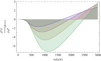
Notice that for given fermion masses, the specific value of the effective self-interaction at the electroweak symmetry breaking scale depends on the value of the unknown scale . Up to this point, a wide range of possible values for the cut-off are eligible and one must take into account the dependence of the parameters of the model on , as we will do in section III. However, these values must be consistent with the perturbative treatment we are using which requires a small effective scalar self-interaction. From Fig. (1) we can see that this narrows the range of values for , the allowed range depending on the specific masses of the fourth generation. Interestingly, for given values of the fermion masses, there are specific values of such that the effective self interaction also vanishes. These specific values are worthy to study in detail because in this case the effects of scalar self-interactions in the EWSB at the next order in perturbation theory also vanish and EWSB is still driven by the Yukawa couplings at that order. Furthermore, in this case the scale is fixed by the electroweak scale and the values of the fermion masses.
There are two solutions to the equation
| (10) |
for heavy fermion masses in the range given in Eqs.(1, 2). One of them yields around the electroweak symmetry breaking scale and we consider it as unphysical. The other solution lies in the range
| (11) |
depending on the input for the masses of the fourth generation fermions.
Once we have fixed the cutoff for given masses of the heavy fermions, we obtain from Eq. (8) the corresponding Higgs mass as a function of the fourth generation quark and lepton masses. In the numerical analysis we use
| (12) |
as suggested by Eqs.(1, 2). Under these considerations, the Higgs mass is a smooth function of and and has a more pronounced dependence on as shown in Figs.(2, 3). More important, a modest Higgs mass of GeV is reachable and even a heavy Higgs of GeV would be consistent with electroweak precision data if EWSB is entirely driven by Yukawa forces of the hypothetical fourth generation and the top quark.

Notice that if fourth generation lepton masses are of order GeV, then the contribution of and almost determine completely the Higgs mass prediction, as depicted in Fig.(2). Combining Eq.(8) and Eq.(1) with condition Eq.(10), this fact is expressed as follows:
| (13) |
Also in this case, the cutoff for new physics should be within the range given in Eq.(11). A simple and good approximation for this case is
| (14) |
with .
It is important to remark that even for masses of the 4th generation around 500 GeV, the corresponding Yukawa couplings () are around thus the loop expansion parameter, given by , is smaller than one and justifies our perturbative approach.
Results contained in Figs.(2, 3) are in agreement –mutatis mutandis– with the analysis performed in the full renormalized SM4 framework [8].

III RG Improved Model
It is important to check the consistency and stability of our previous approach to take into account the running of the Yukawa couplings as it is well known that these couplings could reach the non perturbative regime very quickly. In this section, following the approach of [36] we investigate the leading effects of the heavy fourth generation quarks on the scalar sector with a special emphasis on the perturbative nature of the analysis and its implications on the possible choices for the ultraviolet cut-off. We use the Renormalization Group equation (RG) to estimate the running of the couplings.
From the previous results, we learned that the contribution of gauge bosons, top quark and fourth generation leptons to the one-loop effective potential is negligible compared to that of the fourth generation quarks if we assume that new leptons are relatively light. In a first approximation we will consider only the effects of the running in the fourth family of quarks. In order to incorporate these effects properly in the analysis of the Higgs mass, we will use the pole mass for the Higgs. Furthermore, the study of the perturbative regime will require the running of the fermion masses which are dictated by the running of the Yukawa couplings. Since we will study the behavior of our observables as a function of these masses it is important to work with the fermion masses as defined at the corresponding scale, i.e. . Finally we will incorporate renormalization effects of the vacuum expectation value of the scalar field. All these effects are more easily handled using a more conventional approach thus, unlike the previous section, here we start with the bare Lagrangian whose sector of our primary interest is
| (15) |
with
| (16) |
At one loop level we have
| (17) |
Again, if we insist in a dynamical SB triggered by fourth generation quarks and we set , the only non-trivial solution to is
| (18) |
with for the inputs of the analysis. This means that we have an authentic scalar in the SB sector. Here
| (19) |
with as the “bare” vacuum expectation value, where the subscript denotes the fact that this is an approximation with only the one-loop fourth generation quantum effects.
It is important to notice that our Lagrangian depends now on the values of the coupling at the cut-off scale. In this section the cut-off scale will be defined as the scale where the perturbative regime for the Yukawa couplings is still valid. Above this scale, the Yukawa couplings could get strong enough to generate non-perturbative effects as condensate formation or others.
In order to obtain predictions on physical quantities, we must make an adequate choice of taking special care in the preservation of the perturbative expansion. The relations between the bare parameters of the model and the physical parameters proceed as follows: The physical (pole) mass of the scalar can be expressed in terms of the effective potential as
| (20) | |||||
where stands for the scalar self energy, that can be approximated as the following truncated Green function calculated with fourth generation one-loop effects only
| (21) |
A straightforward calculation performing the Wick rotation in Euclidean space and imposing a spherical cut-off on the euclidean quark momentum yields
| (22) |
In this framework, the relation among the bare VEV and its renormalized counterpart is given by the renormalization of the kinetic scalar term and can be written as
| (23) |
where
| (24) |
In the matter sector, the running of the relevant Yukawa couplings can be summarized in the following Renormalization Group Equations:
| (25) | |||
| (26) |
In the approximation , defining , the previous equations reduce to
| (27) | |||
| (28) |
and the solution can be written as
| (29) |
| (30) |
The physical mass of the heaviest fourth generation quark are defined as
| (31) |
The running of Yukawa couplings from to is given by
| (32) |
| (33) |
Inserting (22) into (20), the squared pole mass of the scalar is
| (34) |
In this case, maximum cut-off can be naturally defined as the largest scale at which the model remains perturbative. That scale is achieved when alpha-Yukawa becomes equal to one
| (35) |
which can be solved to yield
| (36) |
In Fig.(4), is shown as a function of the heaviest quark mass. Hence, for a quark with mass GeV the maximum cut-off is GeV; while for GeV we have GeV. Even in this case, a Higgs mass between GeV and GeV is compatible with fourth generation quarks with masses between GeV and GeV which are responsible for the EWSB in a perturbative fashion with a physical cut-off .
Comparing with the previous section we can see that perturbative effects indeed appear at a lower scale than the naive scale for new physics. Still, taking the worst case, e.g., , the predicted Higgs mass lies in the same range as before and the perturbative expansion is valid up to GeV, where . This is shown explicitly in Fig.(5), where the curve represents the Higgs mass that correspond to the cut-off choice as a function of the mass of the heaviest quark with GeV. Thus, the predictions of the previous model are not strongly modified by the RG Yukawa couplings, but the interpretation of the cutoff scale is different.


IV Dynamical symmetry breaking in MSSM4
We now perform an analogous calculation in the context of a low energy supersymmetric extension of the SM with a fourth generation of chiral matter. As is well known, in the Higgs sector of MSSM there are two scalar doublets of opposite hypercharge: , . Breaking supersymmetry softly, the tree-level scalar potential for the CP-even neutral scalars and is
| (37) |
The linear combination
| (38) |
with diagonalizes the mass matrix in Eq.(37) and the potential becomes
| (39) |
where
| (40) |
Here, as in section II, the parameters of the Lagrangian are identified as the physical ones evaluated at the electroweak scale. If we demand , then only SUSY is broken at tree level -leaving electroweak symmetry untouched- and from Eq. (40) we have . Also, if we require the potential to be bounded from below, the parameters are constrained to satisfy .
As usual in this context, we work in the decoupling limit where all SUSY partners of SM particles and all physical scalars that emerge from the Higgs sector (except for ) are heavy, with masses of the order of the global SUSY breaking scale . From the analysis of the previous section we know that the contribution of gauge bosons and fourth generation leptons to the one-loop effective potential are negligible; in the first case because of the relative smallness of the gauge couplings compared to the quark Yukawa couplings and in the second case because the number of degrees of freedom per lepton is that of quarks. For simplicity, we also discard terms of the form , and because their contribution is also dictated by the gauge couplings. Under these simplifications, the resulting effective potential is given by Eq.(6) with and field-dependent masses , , ,
| (41) |
where . In the above expression we have
| (42) |
with as soft supersymmetry-breaking mass parameters for the left- and right-handed squarks and
| (43) |
Note that the discussion about Yukawa couplings given in the previous section applies in this case to the quantities , and for fixed . In Eq.(41), the parameters control the mixing between squarks in each generation. We assume that there is no mixing, taking . The degrees of freedom per particle are , . Notice also that in this case the tree-level scalar self interactions cannot be taken as zero.
The parameter can be expressed now in terms of the physical masses after the minimization of the effective potential. At one obtains
| (44) |
with again for the present set up. For the Higgs mass and the effective Higgs self-coupling at electroweak scale one has
| (45) |
and
| (46) |
neglecting terms that vanish as because the soft breaking terms for the squarks play the role of natural regulators in this case.
Again, if we insist that electroweak SB is completely produced by quark and squark loops, consistency requires that Higgs self interactions must remain small at least at the scale of SB as in Eq.(10). Taking for all squarks the same soft mass in Eq.(42), one can extract the maximum value of allowed by . This is shown in Fig. (6). The solution turns to be very stable and lies in the range
| (47) |
for with fixed values of , and and the relation Eq.(12) for the masses of the fourth generation quarks. The results turn to be weakly dependent as we will see in Fig. (7).

Finally, once determined the parameter , Eq.(45) leads to the corresponding Higgs mass upper bound in the limit as a function of and as shown in Fig. (7). The prediction for the Higgs mass is very similar to that of the previous section, from GeV to about GeV up to small corrections that would come from gauge bosons, leptons and sleptons in the loop, which are expected to modify our results only a few percent. In fact, even the contribution of top quarks is negligible (see Fig. (7)). From Eq.(45), Eq.(46) and Eq.(10), the dominant contribution to Higgs mass (taking for simplicity, which implies ) is:
| (48) |
with and given by Eq.(47). Given the small difference between and , a good approximation to Eq.(48) is simply
| (49) |
which correspond to and .

V Conclusions
In this paper, we study the possibility of electroweak symmetry breaking by radiative corrections [28] due to a fourth generation in the Standard Model. We isolate the effects of the fourth generation by taking a vanishing scalar self-coupling at the classical level and maintaining this condition valid at one loop level at the electroweak symmetry breaking scale. In such a scenario, electroweak symmetry is broken by radiative corrections due mainly to the fourth generation and Higgs masses of the order of a few hundreds of GeV are consistent with electroweak precision data. Furthermore, the theory is valid only up to a scale TeV. Such low cut-off means that the effects of new physics needed to describe electroweak interactions at energy above should be measurable at the LHC. We use the renormalization group equation to study the impact of the running of the Yukawa couplings in our results. We show that the predictions of the model are not strongly modified by the running of the Yukawa couplings, but a slightly lower cut-off related to the breaking of the perturbative regime is expected in this case.
As an example of models with new physics and therefore containing a natural scale for the cut-off of the electroweak interactions regime, we study a simplified Minimal Supersymmetric Standard Model with four generations. We obtain similar values for the Higgs mass with weak dependence. The natural scale for the cut-off of the electroweak regime is given by the mass of the fourth generation squarks and EWSB by radiative corrections due predominantly to the fourth generation requires masses for the squarks of the order .
VI acknowledgements
This work was supported by CONACyT (Mexico) under grant 50471-F, DINPO-UG and PROMEP-SEP.
References
- [1] S.-W. Lin, Y. Unno, W.-S. Hou, and P. Chang et al. (Belle Collaboration), Nature 452, 332 (2008); B. Aubert et al. (BABAR Collaboration), Phys. Rev. D 76, 091102 (2007); B. Aubert et al. (BABAR Collaboration), arXiv:hep-ex/0807.4226 [hep-ex].
- [2] M. S. Chanowitz, Phys. Rev. Lett. 87, 231802 (2001) [arXiv:hep-ph/0104024]; M. S. Chanowitz, Phys. Rev. D 66, 073002 (2002) [arXiv:hep-ph/0207123].
- [3] M. Maltoni, V. A. Novikov, L. B. Okun, A. N. Rozanov and M. I. Vysotsky, Phys. Lett. B 476, 107 (2000) [arXiv:hep-ph/9911535].
- [4] H. -J. He, N. Polonsky, S. Su, Phys. Rev. D64, 053004 (2001). [hep-ph/0102144].
- [5] V. A. Novikov, L. B. Okun, A. N. Rozanov and M. I. Vysotsky, JETP Lett. 76, 127 (2002) [Pisma Zh. Eksp. Teor. Fiz. 76, 158 (2002)] [arXiv:hep-ph/0203132]; Phys. Lett. B 529, 111 (2002) [arXiv:hep-ph/0111028].
- [6] G. D. Kribs, T. Plehn, M. Spannowsky and T. M. P. Tait, Phys. Rev. D 76, 075016 (2007) [arXiv:0706.3718 [hep-ph]].
- [7] P. Q. Hung and M. Sher, Phys. Rev. D 77, 037302 (2008) [arXiv:0711.4353 [hep-ph]].
- [8] M. Hashimoto, [arXiv:1001.4335 [hep-ph]].
- [9] P. H. Frampton, P. Q. Hung and M. Sher, Phys. Rept. 330, 263 (2000) [arXiv:hep-ph/9903387].
- [10] B. Holdom, W. S. Hou, T. Hurth, M. L. Mangano, S. Sultansoy and G. Unel, PMC Phys. A 3, 4 (2009) [arXiv:0904.4698 [hep-ph]].
- [11] B. Holdom, Phys. Rev. Lett. 57, 2496 (1986) [Erratum-ibid. 58, 177 (1987)].
- [12] C. T. Hill, M. A. Luty and E. A. Paschos, Phys. Rev. D 43, 3011 (1991).
- [13] J. Carpenter, R. Norton, S. Siegemund-Broka and A. Soni, Phys. Rev. Lett. 65, 153 (1990).
- [14] P. Q. Hung and C. Xiong, arXiv:0911.3890 [hep-ph].
- [15] P. Q. Hung, Phys. Rev. Lett. 80, 3000 (1998) [arXiv:hep-ph/9712338].
- [16] S. W. Ham, S. K. Oh and D. Son, Phys. Rev. D 71, 015001 (2005) [arXiv:hep-ph/0411012].
- [17] R. Fok and G. D. Kribs, Phys. Rev. D 78, 075023 (2008) [arXiv:0803.4207 [hep-ph]].
- [18] Y. Kikukawa, M. Kohda and J. Yasuda, Prog. Theor. Phys. 122, 401 (2009) [arXiv:0901.1962 [hep-ph]].
- [19] W. S. Hou, Chin. J. Phys. 47, 134 (2009) [arXiv:0803.1234 [hep-ph]].
- [20] P. Q. Hung and C. Xiong, arXiv:0911.3892 [hep-ph].
- [21] A. Soni, A. K. Alok, A. Giri, R. Mohanta and S. Nandi, arXiv:0807.1971 [hep-ph].
- [22] W. S. Hou, M. Nagashima and A. Soddu, Phys. Rev. Lett. 95, 141601 (2005) [arXiv:hep-ph/0503072]. W.-S. Hou, M. Nagashima, G. Raz, and A. Soddu, J. High Energy Phys. 09 (2006) 012;
- [23] W. S. Hou, H. N. Li, S. Mishima, M. Nagashima, Phys. Rev. Lett. 98, 131801 (2007). [hep-ph/0611107]. W.-S. Hou, M. Nagashima, and A. Soddu, Phys. Rev. D 76, 016004 (2007).
- [24] M. Bobrowski, A. Lenz, J. Riedl and J. Rohrwild, Phys. Rev. D 79, 113006 (2009) [arXiv:0902.4883 [hep-ph]].
- [25] P. Achard et al. [L3 Collaboration], Phys. Lett. B 517, 75 (2001) [arXiv:hep-ex/0107015].
- [26] A. Lister (for the CDF Collaboration), arXiv:hep-exp/0810.3349.
- [27] T. Aaltonen et al. [The CDF Collaboration], arXiv:0912.1057 [hep-ex].
- [28] S. R. Coleman and E. J. Weinberg, Phys. Rev. D 7, 1888 (1973).
- [29] J. P. Fatelo, J. M. Gerard, T. Hambye and J. Weyers, Phys. Rev. Lett. 74, 492 (1995).
- [30] M. Chaichian, R. Gonzalez Felipe and K. Huitu, Phys. Lett. B 363, 101 (1995) [arXiv:hep-ph/9509223].
- [31] J. E. Dubicki and C. D. Froggatt, Phys. Lett. B 567, 46 (2003) [arXiv:hep-ph/0305007].
- [32] M. S. Carena, H. E. Haber and C. E. M. Wagner, Nucl. Phys. B 472, 55 (1996) [arXiv:hep-ph/9512446].
- [33] J. F. Gunion, D. W. McKay and H. Pois, Phys. Rev. D 53, 1616 (1996) [arXiv:hep-ph/9507323].
- [34] I. J. R. Aitchison, A. J. G. Hey, “Gauge theories in particle physics: A practical introduction. Vol. 1: From relativistic quantum mechanics to QED,” Bristol, UK: IOP (2003) page 298.
- [35] M. Sher, Phys. Rept. 179, 273 (1989).
- [36] G. Cvetic, Int. J. Mod. Phys. A 11, 5405 (1996) [arXiv:hep-ph/9509350].