Small Hairy Black Holes in Global AdS Spacetime
Abstract:
We study small charged black holes in global AdS spacetime in the presence of a charged massless minimally coupled scalar field. In a certain parameter range these black holes suffer from well known superradiant instabilities. We demonstrate that the end point of the resultant tachyon condensation process is a hairy black hole which we construct analytically in a perturbative expansion in the black hole radius. At leading order our solution is a small undeformed RNAdS black hole immersed into a charged scalar condensate that fills the AdS ‘box’. These hairy black hole solutions appear in a two parameter family labelled by their mass and charge. Their mass is bounded from below by a function of their charge; at the lower bound a hairy black hole reduces to a regular horizon free soliton which can also be thought of as a nonlinear Bose condensate. We compute the microcanonical phase diagram of our system at small mass, and demonstrate that it exhibits a second order ‘phase transition’ between the RNAdS black hole and the hairy black hole phases.
1 Introduction
There has been much recent interest in the physics of charged black brane solutions of the Lagrangian11 1 We have chosen to work in 5 spacetime dimensions, and chosen the scalar field below to be massless merely for simplicity. The analysis of this paper carries over, without qualitative modification, in arbitrary spacetime and for arbitrary scalar potential.
| (1) |
where is the Newtons’s constant and the radius of AdS5 is set to unity22 2 See Appendix H for a summary of notation employed in this paper.. This system (sometimes called the massless Abelian Higgs model) admits a well known set of charged black brane solutions which are asymptotically Poincare AdS. Recent interest in this system is due to Gubser’s observation [1] that, at large and when they are near enough to extremality, these black branes are unstable . The end point of the tachyon condensation sparked by this instability is a so called hairy black brane - a solution with a planar horizon immersed in a charged scalar condensate. Black branes interacting with such matter condensates are novel and interesting, and have been studied intensively over the last few years (see [2, 3, 4, 5, 6] and references therein). Unfortunately almost all constructions of these solutions have been numerical33 3 See however [7, 8, 9] for analytical studies in a related context..
Under the AdS/CFT correspondence, these planar AdS5 solutions are dual to the states of a conformal field theory living on the flat spacetime . Another natural arena to study dimensional conformal field theories is to work on instead. States of such a boundary field theory living on are dual to gravitational solutions that asymptote to global AdS5 instead of planar AdS5. The corresponding charged black holes in global AdS5 spacetime are characterised by their radius in units of the AdS5 radius and their charge. At large horizon radius, these black holes are locally well approximated by black branes and we expect their physics to be qualitatively similar to the Poincare AdS charged branes. It is natural to enquire about the opposite limit: do small hairy black holes exist, and what are their qualitative properties? In this paper we answer this question by explicitly constructing a set of spherically symmetric hairy charged black holes whose radii are small compared to the AdS5 radius44 4 See [10] for earlier work on scalar condensation in black hole backgrounds in global AdS5.. Our construction is perturbative in the radii of our solutions, but is otherwise analytic. It permits an analytic construction of the microcanonical phase diagram of our system at small mass and charge. In the rest of this introduction, we will describe in detail our construction of small hairy black holes, their properties, and the phase diagram of our system.
To begin with, we start our discussion with a consideration that may, at first, seem unrelated to the study of AdS black holes. Consider a spherically symmetric shell of a scalar field of frequency incident on a charged black hole in flat spacetime. One might naively expect a part of this wave to be absorbed by the black hole while the rest is reflected back to infinity. It is, however, a well known fact that the reflection coefficient for this process actually exceeds unity when ( is the chemical potential of the black hole). Under these conditions more of the incident wave comes out than was sent in. This phenomenon, called superradiance [11], has immediate and well known implications for the stability of small RNAdS black holes, as we now explain.
Consider a superradiant wave incident on a small charged black hole sitting at the centre of global AdS spacetime. Such a wave reflects off the black hole, propagates out to large , but unlike the flat spacetime case, bounces back from the boundary of AdS5 and then finds itself re-incident on the black hole. This process continues indefinitely. As every reflection increases the amplitude of this wave by a fixed factor, this process constitutes an instability of the charged black hole. A closely related instability, the so called black hole bomb, was discussed (in the context of a flat spacetime black hole surrounded by mirrors) as early as the 1970s [12].
As the spectrum of frequencies of a minimally coupled charged scalar field (in a gauge where ) in AdS5 is bounded from below , we expect small charged black holes in AdS5 space to exhibit superradiant instabilities whenever the condition is satisfied55 5 In Appendix A, we verify this expectation by direct computation of the lowest quasi normal mode of this system. We find that for small R, the imaginary part of the frequency of this mode is given by , where is the Schwarzschild radius of the black hole. This imaginary part changes sign precisely where we expect the instability.. Now the chemical potential of a small black hole is bounded from above by the chemical potential of the extremal black hole; i.e. . It follows that small charged AdS black holes are always stable when . When , however, small black holes that are near enough to extremality suffer from a superradiant instability.
The superradiant instability described above admits a very simple thermodynamical interpretation. Notice that the Boltzmann factor for a mode of energy and charge is given by where is the temperature of the black hole. Now this factor leads to an exponential enhancement (rather than the more usual suppression) whenever . In other words, a small charged black hole with is unstable against Bose condensation of the lightest scalar mode. Indeed the leading unstable mode of a small charged black hole with is a small deformation of the lightest scalar mode in global AdS5 space.
The considerations outlined above suggests that superradiant tachyon condensation proceeds in the following manner. The black hole emits into a scalar condensate, thereby losing mass and charge itself. As the charge to mass ratio of the condensate (i.e superradiant mode), , exceeds , the chemical potential of the black hole also decreases as this emission proceeds. Now the decay rate of the black hole is proportional to and so slows down as approaches . It seems intuitively plausible that the system asymptotes to a configuration consisting of a stationary charged black hole core surrounded by a diffuse AdS scale charge condensate, i.e. a hairy black hole. We will provide substantial quantitative evidence for the correctness of this picture in this paper.
In the discussion of the previous paragraph we have ignored both the backreaction of the scalar field on the geometry as well as the effect of the charged black hole core on the scalar condensate. However these effects turn out to be small whenever the starting black hole is small enough. In other words the end point of the superradiant instability of a small charged black hole is given approximately by a non-interacting mix of the black hole core and the condensate cloud at leading order. We will now pause to explain why this is the case.
First note that the charge and energy density of the superradiant mode is contained in an AdS radius scale cloud. As the charge and mass the initial unstable black hole is small, the same is true charge and mass of the eventual the scalar condensate. Consequently, the scalar condensate is of low density and so backreacts only weakly on the geometry everywhere.66 6 Note that, in contrast, for the small charged black hole at the core has its mass and charge concentrated within a small Schwarzschild radius. Consequently even a black hole of very small mass and charge is a large perturbation about the AdS vacuum at length scales comparable to its Schwarzschild radius. For this reason the metric of the final solution is a small deformation of the RNAdS black hole with , and the scalar condensate does not significantly affect the properties of the RNAdS black hole. On the other hand the condensate cloud is very large compared to the RNAdS black hole at its core. This difference in scales ensures that the charged black hole also does not significantly affect the properties of the scalar condensate.
Motivated by these considerations, in this paper we construct the hairy black hole that marks the end point of the superradiant tachyon condensation process in a perturbative expansion around a small RNAdS black hole with and small but arbitrary radius. The perturbative procedure we employ in our construction is completely standard except for one twist, which we now explain. As is usual in perturbation theory, we expand out the metric, gauge field and scalar field in a power series in which is the small parameter of our expansion77 7 As we explain in Section 2 below, we find it convenient to choose to be the coefficient of the decay of the scalar field at infinity, i.e. the vacuum expectation value of the operator dual to the scalar field.
| (2) |
Here and are the metric and gauge field of our starting RNAdS black hole solution. We then plug this expansion into the equations of motion, expand the latter in a power series in , and attempt to solve the resultant equations recursively. Unfortunately, the linear ordinary differential equations that appear in this process do not appear to be analytically solvable in full generality. However it turns out to be easy to solve these equations separately in two regimes: at large (in an expansion in which we call as the far-field expansion and mark by a superscript ‘out’) and at small (in an expansion in which we call the near-field expansion and mark by a superscript ’in’). Here is the radial coordinate (that is zero at the black hole singularity and infinity at the boundary of AdS ) and is the Schwarzschild radius of the unperturbed RNAdS black hole solution. The first expansion is valid when , while the second expansion works when . As we are interested in , the validity domains of these two approximations overlap. Consequently, we are able to solve the resultant linear equations everywhere, in a power series expansion in .
When the dust has settled we are thus able to solve for the hairy black holes only in a double expansion in and . This expansion is sufficient to understand small hairy black holes 88 8 The technical obstruction to solving the equations at arbitrary has a physical interpretation. Even at arbitrarily small , the black hole reacts significantly on the condensate at finite . Our system can be regarded as a non interacting mix of the black hole and the condensate only at very small . Effectively, in this paper, we perturb around this non interacting limit.. In section 2 below we have explicitly implemented this expansion to for . Our calculations allow us to determine the microcanonical phase diagram of our system, as a function of mass and charge at small values of these parameters99 9 The microcanonical ensemble is well suited to our purposes. We discuss the phase diagram in other ensembles, in particular the canonical and grand canonical ensemble, in Appendix F and G below. We are able to make less definite statements in these ensembles because it turns out that the system at a given fixed chemical potential and temperature often receives contributions both from small as well as big black holes. As the approximation techniques of this paper do not apply to big black holes, we are unable to quantitatively assess the relative importance of these saddle points.; our results are plotted for in Fig.1 below (the results are qualitatively similar for every provided , and may also be simply generalised to the study of (1) with a mass term added for the scalar field- see 6.4).
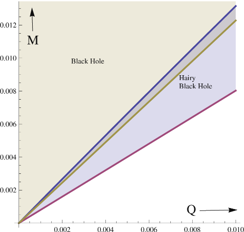
As summarised in Fig.1, hairy black holes exist only in the mass range
| (3) |
where and are the mass and the charge of the hairy black hole.
Above the upper bound in (3) (i.e. in the shaded grey region above the blue line in Fig.1.), RNAdS black holes are stable and are the only known stationary solutions. The upper end of (3) coincides with the onset of superradiant instabilities for RNAdS black holes. The lower bound in (3) is marked by the lowest (i.e. red) line in Fig.1. The extremality line for RNAdS black holes (the yellow line in Fig.1.) lies in the middle of this range in (3). At masses below lower bound of (3) (red line in Fig.1.), the system presumably has no states.
As we have emphasised, a hairy black hole may approximately be thought of as a non interacting superposition of a RNAdS black hole and a scalar Bose condensate. At the upper bound of (3) the condensate vanishes, and hairy black holes reduce to a RNAdS black holes. As we decrease the mass of a hairy black hole at fixed charge (or increase the charge at fixed mass), the fraction of the condensate increases. Eventually, at the lower end of (3) - the red line in Fig.1. - the black hole shrinks to zero. In this limit 1010 10 We take the limit purely within classical relativity. Of course stringy and quantum gravity effects (including the one loop energy density of the gas outside the black hole) become important when the black hole becomes parametrically small. Such effects are important only in an infinitesimal wedge above the red line in Fig. 1 and depend on the detailed microphysics of the system (they would be different, for instance, in string theory and M theory). We ignore all such effects in this paper. We thank K. Papadodimas for a discussion on this issue. the solution reduces to a regular horizon free soliton (see [13] for the appearance of a similar solitonic solution in a qualitatively similar context). The solitonic solution, on the red line of Fig.1 is simpler than the hairy black hole solution. As on this solution, it may be generated as an expansion in a single parameter ; in Appendix C we have carried out this expansion to 17th order. Hairy black holes may be thought of as solitons with small RNAdS solutions in their centre (see the related general analysis1111 11 We thank G. Horowitz and H. Reall for drawing our attention to this reference. of [14] ).
In summary, the hairy black hole interpolates between pure black hole and pure condensate as we scan from the upper to the lower bound of (3) (or down from the blue line to the red line in Fig.1.).Throughout the range of its existence, the hairy black hole is the only known stable solution1212 12 Except for excited solitons, see below for details.. It is also the thermodynamically dominant solution, as the entropy of the hairy black hole exceeds that of the RNAdS black hole of the same mass and charge, whenever both solutions exist.
Note that the solitonic solutions described above have some similarities to so called boson stars1313 13 We thank G. Horowitz, M. Rangamani and K. Papadodimas for drawing our attention to the literature on boson stars and explaining their properties to us. K. Papadodimas has further drawn our attention to the fact that our soliton reduces precisely to a traditional boson star in the limit . Of course hairy black holes exist only when and so do not exist in the small limit., which have been extensively discussed in the General Relativity literature, mainly in asymptotically flat space (see e.g. [15]) but also in asymptotically AdS spaces (see e.g. [16]). However boson stars usually have scalar fields with a harmonic time dependence, which obstructs placing black holes in their centre (the scalar field would oscillate an infinite number of times as it approaches the horizon). Our solitonic solutions are genuinely stationary1414 14 The presence of the gauge field allows us to evade Derrick’s theorem. We thank K. Papadodimas pointing this out. in a particular gauge. In this gauge the temporal component of the gauge field takes a particular non zero value at the origin of the soliton. This allows us to construct stationary hairy black hole solutions by placing charged black holes at the centre of the soliton (roughly via the procedure of [14].) if and only if the black holes are chosen so that their chemical potential matches the gauge field at the centre of the soliton. The last condition has a simple and intuitive thermodynamical interpretation; solitons and black holes can be put into an approximately non interacting mix only when their chemical potentials match!
The hairy black hole we have described so far in this introduction is a weakly interacting mix of the RNAdS black hole and a condensate of the ground state of the scalar field. The reader may wonder whether it is possible to construct an excited hairy black hole solution that is a weakly interacting mix of a RNAdS black hole and an excited state of the scalar field. This is indeed the case. The set of spherically symmetric linearised excitations of a massless scalar field appear in a one parameter family1515 15 These modes are dual, under the state operator map, to the operator , where is the dimension 4 operator that corresponds to the bulk field according to the rules of the AdS/CFT dictionary. labelled by an integer . The energy of the state is where . It turns out to be possible to mimic the construction described above to construct excited hairy black holes that reduce, at small masses, to the superposition of a RNAdS black hole with with a condensate of the scalar excited state. It turns out that these excited hairy black holes are all unstable to the superradiant decay of the scalar mode with energy . They presumably decay to the ground state hairy black hole, in comparison to which they are all turn out to be entropically sub dominant.
Each excited hairy black hole exists in a limited mass range which turns out to be a subset of the mass range (3). At the lower end of this range, each excited hairy black hole reduces to a horizon free scalar condensate, i.e. an excited soliton. Here we find a surprise. Recall that the instability of excited state hairy black holes is superradiant in nature. Superradiant instability rates scale like , and so go to zero as . It thus appears that excited state scalars are actually stable to small fluctuations, and so cannot decay classically. The discussion of this paragraph actually leaves open the possibility that excited solitons may have an independent non super radiant instability mode. It is, however, possible to demonstrate that the spectrum of small oscillations about arbitrary unstable solitons has no exponentially growing eigenmode, at least within the assumption of spherical symmetry (see 6.3). While this result does not rigorously prove the stability of excited solitons [17, 18], it at least suggests that they are stable. We find this surprising and do not have a clear sense for its implications.
It may be worth pausing to consider the relative merits and disadvantages of the perturbative procedure of this paper versus the numerical approach more usually used to study hairy black branes. On the negative side our perturbative procedure gives us no information about the regime of large masses and charges (where the perturbative expansion breaks down). Within its regime of validity, however, our perturbative procedure is very powerful. It allows us, once and for all, to compute the phase diagram and thermodynamics of all relevant solutions - including each of the infinite number of excited state hairy black holes - as analytic function of the parameters of the problem (e.g. the mass and charge of the scalar field). Perhaps more importantly our procedure gives us qualitative intuitive insight into the nature of hairy black holes. For instance, as we have explained many times, the hairy black hole is an approximately non interacting mix of a RN-AdS black hole and the scalar condensate. This picture together with a few lines of algebra, immediately yields a formula for the entropy of the hairy black hole, to leading order in its mass and charge (see 6.4). In other words the perturbative approach employed in this paper gives more than numerical answers; it helps us to understand why small hairy black holes behave the way they do.
In this paper we have focussed on the black holes in global AdS at small mass and charge. Almost all previous studies of the Lagrangian (1) have studied the system in the Poincare patch1616 16 See however [10] for a study in global AdS. .The local dynamics of black holes in global AdS reduces to the dynamics of black branes of Poincare AdS at large mass and charge. It follows that the phase diagram displayed in Fig.1 should make contact with the results of previous analyses at large mass and charge. In section 7 we present a conjectural phase diagram that interpolates between the small mass and charge behaviour derived in this paper and the large mass and charge behaviour determined in previous work. The analysis of that section makes it clear that something special happens to the phase diagram of hairy at charges, in units of the inverse Newton constant, of order unity. We leave the detailed study of this special behaviour to future work.
The reader who is interested in asymptotically AdS gravitational dynamics principally because of the AdS/CFT correspondence might legitimately complain that our choice of the Lagrangian (1) was arbitrary; the dynamics of charged scalar fields in any given example of the AdS/CFT correspondence is unlikely to be given by (1). Our attitude to this is the following: we regard (1) as a toy model which we have chosen to study (in common with much earlier work on the subject), largely because it is a simple system that possesses several of the ingredients that are qualitatively important for hairy black hole dynamics. Our exhaustive study in this paper of the toy model sets the stage for a similar analysis of small hairy black holes in ‘realistic’ theories IIB theory on AdS. We expect small of black holes in this special bulk theory to share many of the qualitative features discussed in this paper, but also to have some properties that result from dynamical features special to it. We have already commenced this study and hope to report on it in the near future. 1717 17 In this context it is however important to keep in mind that small black holes in IIB theory on sometimes suffer from Gregory Laflamme instabilities [19] (in addition to potential superradiant instabilities), an additional feature that complicates (but enriches) the dynamics of small black holes in a ‘realistic’ theory like IIB SUGRA on .
Note added in v2 : After the first version of this paper appeared, we became aware of a recent work by Maeda.et.al.[20] studying a similar subject.
2 The basic setup for the Hairy BHs
2.1 Basic equations of motion
As mentioned in the introduction, in this paper we study the Lagrangian (1). This action describes the interaction of a massless minimally coupled scalar field, of charge , interacting with a negative cosmological constant Einstein Maxwell system. Through most of this paper we will be interested in stationary, spherically symmetric solutions of this system . However, in Appendix.A we will generalise to the study of time-dependent configurations to investigate the stability against small fluctuations. We adopt a Schwarzschild like gauge and set
| (4) |
The four unknown functions , , and are constrained by Einstein’s equations, the Maxwell equations and the minimally coupled scalar equations. It is possible to demonstrate that are solutions to the equations of motion if and only if
| (5) |
The four equations listed in (5) are the and components of Einstein’s equations, the Maxwell equation and the minimally coupled scalar equation, in that order.
The equations (5) contain only first derivatives of and , but depend on derivatives upto the second order for and . It follows that (5) admit a 6 parameter set of solutions. One of these solutions is empty AdS5 space, given by , , . We are interested in those solutions to (5) that asymptote to AdS spacetime, i.e. solutions whose large behaviour is given by
| (6) |
It turns out that these conditions effectively impose two conditions on the solutions of (5), so that the system of equations admits a four parameter set of asymptotically AdS solutions1818 18 For example, the equations above are easily solved in linearisation about AdS5 ;the six dimensional solution space is given by (7) The asymptotically AdS condition set . . We will also be interested in solutions that are regular (in a suitable sense) in the interior. As we will see below, this requirement will cut down solution space to distinct classes of two parameter space of solutions (the parameters may be thought of as the mass and charge of the solutions). In particular, we are seeking the hairy black hole solutions of the above equations that constitute the endpoint of the superradiant instability of small RNAdS black holes. To set the stage and notations for our computation we first briefly review the charged RNAdS black hole solutions in global AdS spacetime.
2.2 RNAdS Black Holes and their superradiance
The AdS-Reissner-Nordstrom black holes constitute a very well known two parameter set of solutions to the equations (5). These solutions are given by
| (8) |
where is the chemical potential of the RNAdS black hole. The function in (8) vanishes at and consequently this solution has a horizon at . In fact, it can be shown that is the outer event horizon provided
| (9) |
We will review later the thermodynamics of these solutions in more detail with a particular focus on small charged black holes whose . Consider the small RNAdS black hole solutions of the system described by the Lagrangian in (1). As we have explained in the introduction, in the limit we expect the solution in (8) to be unstable to superradiant decay provided . In appendix A, we verify this intuitive expectation by determining the lowest quasinormal mode of this system in a power series in . In a gauge where , we find that the time dependence of this lowest mode is given by where
| (10) |
Note in particular that
it follows that the time dependence of this mode represents an exponential damping when but an exponential growth when . Consequently, small charged black holes are unstable when , in agreement with the intuitive expectations outlined in the introduction. Further, note that the decay (or growth) constant of the lowest quasi normal mode is given by , and goes to zero either when goes to zero or as goes near . As we have argued in the introduction, this motivates us to seek a hairy black hole solution which is constructed in a perturbation theory about these RNAdS blackholes.
2.3 Setting up the perturbation theory
The starting point of our construction is a small RNAdS black hole
| (11) |
at arbitrary but small , and
| (12) |
Here is the as yet unknown chemical potential of our final solution. Note that, at the leading order in the perturbative expansion, .
To proceed we simply expand every unknown function
| (13) |
Here , and are the values of the functions , and for a RNAdS black hole with radius and chemical potential . given in (12). We expand our equations in a power series in . At each order in we have a set of linear differential equations (see below for the explicit form of the equations), which we solve subject to the requirements of the normalisability of and at infinity together with the regularity of and the metric at the horizon. These four physical requirements turn out to automatically imply that i.e. the gauge field vanishes at the horizon, as we would expect of a stationary solution. These four physical requirements determine 4 of the six integration constants in the differential equation, yielding a two parameter set of solutions. We fix the remaining two integration constants by adopting the following conventions to label our solutions: we require that fall off at infinity like (definition of ), that the horizon area of our solution is (definition of ). This procedure completely determines our solution as a function of and . We can then read of the value of in (12) on our solution from the value of the gauge field at infinity.
As we have explained in the introduction, the linear differential equations that arise in perturbation theory are difficult to solve exactly, but are easily solved in a power series expansion in , by matching near field and far field solutions. At every order in we thus have a solution as an expansion in . Our final solutions are, then presented in a double power series expansion in and .
In the next few sections, we present a detailed description of the implementation of this perturbation expansion at order and . In Appendix B we present explicit results for this perturbation expansion at higher orders.
3 Perturbation theory at
We will now present a detailed description of the implementation of our perturbative expansion at . The procedure described in this subsection applies, with minor modifications, to the perturbative construction at for all .
In this section we wish to construct the first order correction around the black hole
| (14) |
Plugging in (13), we expand the equations of motion in a power series in to . Of course all equations are automatically obeyed at . The only nontrivial equation at is where is the linearised gauge covariantised Laplace equation about the background (14). We will now solve this equation subject to the constraints of normalisability at infinity, regularity at the horizon, and the requirement that at large .
3.1 Far Field Region
Let us first focus on the region . In this region the background (14) is a small perturbation about global AdS space. For this reason we expand
| (15) |
where the superscript out emphasises that this expansion is good at large . In the limit , (14) reduces to global AdS spacetime with . A stationary linearised fluctuation about this background is gauge equivalent to a linearised fluctuation with time dependence about global AdS space with ( is the temporal component of the gauge field). The required solution is simply the ground state excitation of a massless minimally coupled scalar field about global AdS
| (16) |
The overall normalisation of the mode is set by the requirement
We now plug (15) into the equations of motion and expand to to solve for . Here is the gauge covariant Laplacian about the background (11). Now
where is the gauge covariant Laplacian about global AdS spacetime with background gauge field . It follows that, at ,
This equation is easily integrated and we find
| (17) |
We could iterate this process to generate till any desired . As in (17), it turns out that the expressions are increasingly singular as . In fact it may be shown that the most singular piece of scales like , upto logarithmic corrections. In other words the expansion of in powers of is really an expansion in (upto log corrections) and breaks down at .
In summary we have found that, to
| (18) |
The small expansion of this result is given by
| (19) |
Note that this result depends on the as yet unknown parameter . This quantity will be determined below by matching with the near field solution.
3.2 Near Field Region
Let us now turn to inner region . Over these length scales the small black hole is far from a small perturbation about AdS5 space. Instead the simplification in this region arises from the fact that background gauge field, which is of order unity, is negligible compared to the mass scale set by the horizon radius . In other words the gauge field is a small perturbation about the black hole background in this region. To display this fact it is convenient to work in a rescaled radial coordinate and a rescaled time coordinate . Note that the near field region consists of spacetime points with of order unity. In these coordinates the background black hole solution takes the form
| (20) |
The explicit factor of in in (20) demonstrates the effective weakness of the gauge field. This justifies an expansion of the near field solution in a power series in
| (21) |
To determine the unknown functions in this expansion, we must solve the equation , where is the gauge covariant Laplacian about the background (20). Our solutions are subject to the constraint of regularity at the horizon. Further, they must match with the far field expansion in equations (18) and (19) above.
Note
where in is the leading part of in an R expansion. At leading order we find The two linearly independent solutions of this equation are easily obtained by integration. The only solution regular at the horizon is the constant
where we have determined the value of the constant by matching with equations (18) and (19) (more below about the matching).
At next order in we obtain an equation of the form
Even though is a constant, the RHS of this equation is nonzero because of the gauge field in (14). The equation is easily solved by integration; imposing regularity of the solution at the horizon we find1919 19 The apparent logarithmic singularities at , in two of the terms of (22), actually cancel.
| (22) |
where is the polylog function as defined in Mathematica 6
The single unknown parameter in this solution will be determined by matching below.
The perturbative procedure described above may be iterated to arbitrary order. It turns out that the fields at high are increasingly singular at large . In fact it may be shown that the dominant growth of is generically . It follows that the near field perturbative expansion is an expansion in .
In summary
| (23) |
The large expansion of this result is given by
| (24) |
In (24) we have determined in terms of the as yet unknown parameter which will be determined by matching below.
3.3 Matching
In order to match the near and far field results, we substitute in (24) (the large expansion of ) and view the resultant expression as an expansion about small and small . As we have explained above, the resultant expression is reliable to all order in but only to order ; all terms of order or higher receive contributions from as yet undetermined fourth order terms in the perturbation expansion of (24).
We then compare this expression with the small expansion of , (19). We can generate this expansion to any order in that we desire (merely by Taylor expanding (19)); however the resultant expression is clearly valid only to in (terms of obviously receive contributions from as yet undetermined fourth order terms in the expansion of ). Terms of the form , and (together with logarithmic corrections) are reliably computed by both expansions and so must agree. The unknown parameters and are determined to ensure this (as we have more conditions than variables we also obtain valuable consistency checks). We find
This completes our determination of our solution to . The procedure described in this subsubsection can be iterated to obtain the solution at higher orders.
4 Perturbation theory at
We now briefly outline the procedure used to evaluate the solution at . We proceed in close imitation to the previous subsection. The main difference is that at this (and all even orders) in the expansion, perturbation theory serves to determine the corrections to the functions , and rather than the function . The procedure described here applies, with minor modifications, to the perturbative construction at for all .
4.1 Far Field Region
In the far field region we expand
| (25) |
Plugging this expansion into the equations of motion and expanding to we find equations of the form
| (26) |
Where are the source terms at order which are obtained from terms quadratic in . The most general normalisable solution to these equations takes the form
| (27) |
Note that this solution has three undetermined integration constants and .
Let us first focus on . The constants and are determined by the requirement that the expansion of and at small starts out regular (i.e. has no term that goes like ). This requirement follows from matching with the near field solution. For example, a term in results would match onto a term in that scales like . However has a regular power series expansion in and so does not have such a term 2020 20 At higher orders in the expansion in , similar reasoning will not set and to zero but will instead determine them by matching with . . The constant , is as yet undetermined.
4.2 Near Field Region
We now turn to the solution in the inner region . As in the previous section we find it convenient to solve the equations here in the rescaled and coordinates. We expand
| (28) |
The equations are slightly simpler when rewritten in terms of a new function
where
In terms of this function the final set of equations take the following form.
| (29) |
Where are the source terms which depend on the solutions at all previous orders. The most general solution to these equations is given by
| (30) |
In the above solution two of the four integration constants are chosen such that the solution obeys the requirement that vanishes at the horizon (regularity of the gauge field at the horizon in Euclidean space) and that (this is the requirement that the horizon is located at , which follows from our definition of ). It may also be shown that the remaining two constants in the inner solution at may be determined by matching to the outer solution at the same order ().
In particular, the inner solution at order is completely determined by matching with the outer solution that we have already determined above, in terms of a single unknown . This yields the complete solution at order in terms of this one unknown number.
4.3 Iteration
This process may now be iterated. Our determination of the inner solution at permits an unambiguous determination of the integration constants in the outer solution at . This then allows the complete determination of the inner solution at , which, in turn, permits the determination of the outer solution at and so on. This procedure may be iterated indefinitely.
In summary the procedure described in this subsection permits the complete determination of the correction to our solution (order by order in ), as a function of the shift in the chemical potential at , i.e. in terms of the as yet unknown numbers . These numbers are left undetermined by analysis, but turn out to be fixed by the requirement that there exist regular solutions of the scalar equation at . This is completely analogous to the fact that the shift in the chemical potential was determined from the analysis of the scalar equation at .
It is relatively straightforward (though increasingly tedious) to carry out our perturbative expansion to higher orders in perturbation theory. The equations at odd orders in the expansion serve to determine scalar field corrections, while equations at even orders serve to determine corrections to the metric and gauge field. In Appendix B we list explicit results for the correction to the metric, gauge field and scalar field at low orders in perturbation theory. We will analyse the thermodynamics of these hairy black holes in more detail in later sections.
5 The Soliton
The hairy black hole solitons of the previous section appear in a two parameter family labelled by and . In general our solutions may be thought of as a small RNAdS black hole surrounded by a cloud of scalar condensate. As we have described in the introduction, the limit switches off the condensate cloud. In this limit (the blue line of Fig. 1) hairy black holes reduce to RNAdS black holes. On the other hand, in the limit the black hole at the centre of the condensate cloud shrinks to zero size, apparently leaving behind a horizon free scalar cloud. This is indeed the case. Indeed the solitonic solutions so obtained are considerably simpler than hairy black holes, as they may be generated as a single expansion in . The linear differential equations that we encounter at every order in this process are exactly solvable without recourse to the elaborate matching procedure described in the previous section.
In this section we will directly construct the hairy black hole at in a perturbation expansion in . We refer to the solution of this section as the ‘soliton’. In order to construct the soliton, we search for all stationary charged solutions that are everywhere completely singularity (and horizon) free. We use global AdS as a starting point for these solutions, which we construct in a perturbative expansion in the scalar amplitude. As in the previous section we will only study rotationally invariant solutions, i.e. solutions that preserve the full symmetry group of AdS5 .
At linear order the complete set of regular, asymptotically AdS5 , symmetric fluctuations about global AdS is given by2121 21 We remind the reader that the Gauss’s hypergeometric function is a solution to the equation defined by the series where the ‘Pochhammer symbol’ is defined by the raising factorial Note also that for n an integer, the function is actually an n-th degree polynomial in the variable .
| (31) |
The equation (31) is simply the most general rotationally invariant normalisable and regular solution to the equation . The constant in (31) can be set to any desired value by a choice of gauge. While (31) is generically time dependent, it reduces to a stationary solution when only one of the modes is turned on and is chosen accordingly.i.e.,
for some non-negative integer k. This yields a discrete set of stationary, one parameter, solutions to the equations of motion, labelled by their amplitude. In the rest of this section we describe the construction of the nonlinear counterparts of these solutions in a power series expansion in the amplitude. We refer to these stationary solutions as nonlinear ‘solitons’.
Unlike the two parameter set of black hole solutions described in the previous section, the solitonic solutions of this subsection appear in a one parameter family, labelled by their charge; the soliton mass is a determined function of its charge. The fact that their are fewer solitonic than black hole solutions is related to the fact that the solitons we construct in this subsection have no horizons, and therefore carry no macroscopic entropy.
The ground state soliton (i.e. the soliton at ) has a specially simple interpretation. It may be thought of as the nonlinear version of the Bose condensate, that forms when a macroscopic number of scalar photons each occupies the scalar ground state ‘wave function’. It also represents the limit of the hairy black hole solution of the previous section. We will construct this solution in this section, postponing discussion of excited solitons to the next section.
5.1 Perturbation theory for soliton
To initiate the perturbative construction of the ground state soliton we set
| (32) |
and plug these expansions into (5). We then expand out and solve these equations order by order in . All equations are automatically solved upto . At order the last equation in (5) is trivial while the first three take the form
| (33) |
On the other hand, at order the first three equations in (5) is trivial while the last equation reduces to
| (34) |
Here the source terms are the source terms which are completely determined by the solution to lower orders in perturbation theory, and so should be thought of as known functions, in terms of which we wish to determine the unknowns , , and .
Note that (33) are identical to the equations that appear in the far field expansion of the hairy black hole solution of the previous section. This is intuitive; in the limit all of the hairy black hole spacetime lies within the far field region. The soliton is simpler to construct than the hairy black hole precisely because it has no separate near field region. The differential equations that arise, at any given order of perturbation theory, may simply be solved once and for all, with no need for an elaborate matching procedure.
The equations (33) are all easily integrated. It also turns out that all the integration constants in these equations are uniquely determined by the requirements of regularity, normalisability and our definition of , as we now explain.
The integration constant in the first equation of (33) is determined by the requirement that is regular at the origin. The integration constant in the second equation is fixed by requirement of normalisability for . The constant for the first of the two integrals needed to solve the third equation is fixed by the regularity of at the origin. The constant in the second integral (an additive shift in ) is left unfixed at but is fixed at (see below).
The equation (34) is also easily solved by integration. The constant in the first integration needed to solve this equation is determined by the requirement of regularity of at the origin. Once we have fixed this constant, it turns out that the solution for is generically non normalisable for every value of the second integration constant. In fact normalisability is achieved only when the previously undetermined constant shift of takes a specific value, a condition that determines this quantity. The constant in the last integral that determines from (34) is determined by our definition of which implies that
for .
5.2 Soliton upto
In summary, the perturbative procedure outlined in this subsection is very easily implemented to arbitrary order in perturbation theory. In fact, by automating the procedure described above, we have implemented this perturbative series to 17th order in a Mathematica programme.
We present some of the results, to this order, in Appendix C. In the rest of this subsection we content ourselves with a presentation of our results to .
| (35) |
| (36) |
| (37) |
| (38) |
We will postpone the discussion of the thermodynamics of these solution for later.
5.3 Excited state solitons and hairy BHs
As explained around (31), the stationary solitonic solution constructed in the previous section is simply one (albeit a special one, as it has the smallest mass to charge ratio) of an infinite class of stationary solitonic solutions, each of which may be constructed in a perturbative expansion in , exactly as in the previous section. We label solitonic solutions by an integer ; the stationary soliton has chemical potential at small amplitude.
We have explicitly constructed the excited solitons with and upto a high order in perturbation theory. In Appendix D below we present some of the details of our results at low orders. Further, we can further construct a large class of excited hairy black holes which reduce to these excited state solitons as their horizon size goes to zero. These black holes may be thought of as a mixture of the excited solitons and a small RNAdS black holes with . In Appendix.E, we construct this excited state hairy black hole at . We have a simple program in Mathematica that may be used to generate the excited hairy black hole solution at any fixed value of . It should prove possible to generalise this construction once and for all at arbitrary , but we have not attempted this generalisation. We will present a detailed analysis of the thermodynamics (and stability) of the excited solitons ad black holes later in the paper.
6 Thermodynamics in the Micro Canonical Ensemble
In this section we compare the entropies of the various solutions constructed in this paper as a function of their mass and charge. We find it convenient to present all formulae in terms of the rescaled mass and the rescaled charge . The physical mass and charge of the system, and , differ from and by the rescaling
| (39) |
The grand canonical partition function for the system is defined by the formula
where is the temperature and is the chemical potential.
6.1 RNAdS Black Hole
The basic thermodynamics for an RNAdS blackhole is summarised by the following formulae2222 22 Throughout this paper, we find it convenient to consistently omit a factor of from all our extensive quantities.
| (40) |
were is the charge, is the mass of the black hole, is its entropy, its temperature and its chemical potential.We use the symbol to denote the area of the outer horizon. The condition for to be the outer horizon radius is
| (41) |
We are mainly interested in small RNAdS black holes with . and the thermodynamic expressions can be simplified in this limit. The mass of RNAdS black holes at fixed charge is bounded from below; at small and , we have
For every pair that obeys this inequality, there exists a unique black hole solution.
At small mass and charge (with mass and charge taken to be of the same order) the entropy and the radius of the black hole is given by
| (42) |
At leading order in mass and charge, the chemical potentials of these black holes are given as solutions to the equation
| (43) |
while the temperature is given by
| (44) |
where is given in (42).
6.2 Soliton - Ground State and Excited states
Using the soliton solution in the previous section, the mass of the ground state soliton can be easily determined as a function of its charge. We find
| (45) |
In Appendix C.1, we give the relation of the mass and the charge implicitly upto higher orders.
Upon continuing to Euclidean space, our soliton yields a regular solution for arbitrary periodicity of the Euclidean time coordinate (it is similar to global AdS spacetime in this respect). It follows that, within the classical gravity approximation, this soliton can be in thermodynamical equilibrium at arbitrary temperature. As the soliton has no horizon, its entropy vanishes in the classical gravity approximation. This implies that the free energy of the soliton is equal to its mass.
The chemical potential of the soliton is given by the value of the gauge potential at infinity
| (46) |
Note that the coefficient of in the formula above is positive when so that the chemical potential of the soliton increases with charge whenever hairy black holes exist. It is plausible that the only classical gravity state in the system with is the vacuum (or more precisely a thermal gas about the vacuum; this gas is absent in classical gravity).
The grand free energy of the ground state soliton is given by
| (47) |
The above analysis is easily generalised to excited state solitons. For the general excited state solitons, we present thermodynamical formulae only at leading order. The mass and chemical potential of the soliton are given by
| (48) |
We have explicitly constructed the excited solitons with and upto a high order in perturbation theory. In Appendix D we present some of the details of our results at low orders. This allows us to give the thermodynamic formulae for these cases upto a higher order At we find
| (49) |
while at
| (50) |
Note that the coefficient of in the expansion of in the expansion of (49) is positive whenever so that the first excited hairy black hole exists. On the other hand, the coefficient of in the expansion of is negative at , the threshold for the existence of the second excited hairy black hole (see below).
6.3 Dynamical Stability of solitons
In this subsection, we comment on the dynamical stability of the excited solitons. In particular we will prove below that the spectrum of small fluctuations about excited solitons have no symmetric exponentially growing modes, within the perturbative expansion. This result suggests (but does not strictly prove [17, 18]) that small excited state solitons are all dynamically stable against small fluctuations.
As we have mentioned above, the normal modes of the scalar field constitute the only symmetric fluctuations of (1) about global AdS spacetime. At small the solitonic solution is everywhere a small perturbation around global AdS spacetime. It follows that the symmetric perturbations about the soliton, at small , are small perturbations of spherically symmetric scalar normal modes about global AdS spacetime. These modes obey the equation
| (51) |
where is the gauge covariant derivative about the soliton background. We study perturbations of the form
and wish to investigate whether the frequencies (which are all real about global AdS ) can develop a small imaginary piece about the solitonic background. We will now demonstrate that this is impossible in the expansion. To establish this we multiply the equation (51) by and integrate the resultant scalar over AdS spacetime. We find
Here is the soliton metric and is the gauge field of the solitonic solution.
Now recall that . It follows that
As the leading term on the RHS is and positive, it follows that is real within the expansion. Consequently the spectrum of spherically symmetric small fluctuations about the soliton background does not have exponentially growing modes in the expansion. This suggests that all excited solitons are classically stable. We find this result surprising, and think that it warrants further study.
6.4 Massive scalar : Hairy black hole thermodynamics
We concluded at the end of the previous subsection that the excited solitons seem to be classically stable. In contrast, our calculations in the appendix A indicate that the RNAdS blackhole can become superradiantly unstable. It is an interesting question to ask what is the thermodynamics of the resultant hairy black hole. Since, we have an explicit construction of the hairy black hole solutions, we can directly go ahead to compute the thermodynamic quantities for these hairy solutions. Before doing that however we wish to present an argument in this subsection which gives us some intuition about the kind of thermodynamics we should expect at the leading order.
We will present this argument in a slightly more general framework than we have been working till now - we wish to consider the effect of adding a scalar mass term to the Lagrangian(1).,i.e., we work with a more general system
| (52) |
This system has a minimally coupled charge scalar with mass and charge in AdS5. By the standard rules of AdS/CFT, the dual boundary operator has a scaling dimension
In a gauge where , this is also the energy of the lowest mode in vacuum AdS5. For the case , this reduces to .
The other spherically symmetric modes of (dual to the descendants )have an energy
For the case , . Hence, in a gauge where , the energy of the n-th excited state is also given by . We can form a non-linear Bose condensate by dumping a charge into this n-th excited state - this is equivalent to populating this excited state with number of charged Bosons. To the leading order, where we neglect self-interaction between these Bosons, the mass of such a soliton is given by
This sets the chemical potential of the soliton to be
The entropy of such a solution is zero . This in particular means that within this approximation, this solution exists at arbitrary temperatures .
Now, let us form a hairy black-hole by placing at the core of this non-linear Bose condensate a small ordinary RNAdS black hole with a small outer horizon radius and chemical potential . Such a black hole has a mass
a charge
an entropy
and a temperature
If the number of Bosons is small, then the condensate outside is a small perturbation on the RNAdS black hole. And if the radius of the blackhole is small, then it is a small perturbation on the soliton on length scales large compared to . Hence, if both these conditions are met, it is legitimate at the leading order to assume that there is no interaction between the core and the condensate parts of the hairy black hole. In this regime, since the core and the condensate can still exchange charge and energy, all that is needed for a stationary solution is that the core and the condensate be at a thermal and chemical equilibrium,i.e.,
and
Using these equilibrium conditions we want to figure out the ‘mole fractions’ of these two phases at equilibrium as a function of total mass and charge
This is easily done and we get the mass fractions of the core and the condensate are given by
| (53) |
The charge fractions of the core and the condensate are given by
| (54) |
The radius of the black hole at the core is
| (55) |
and the entropy of the hairy black hole is given by
| (56) |
The existence region of the hairy black holes is in between where the hairy black hole coincides with the RNAdS black hole on one side and where it coincides with the pure soliton on the other side. This gives the existence region as
| (57) |
and this happens only if
where is the critical charge above which the pure black hole becomes superradiantly unstable to radiation in the n-th excited state.
In this regime, the upper bound on is a decreasing function of whereas the lower bound is an increasing function of . This implies that the existence region of n-th excited state hairy black hole is entirely inside the existence region of (n-1)th excited state black hole (see Figure.2). Further, in this regime, one can show that the radius is a decreasing function of . Hence, the higher excited state hairy black holes have smaller cores and consequently are entropically subdominant to the lower excited state hairy black holes.
Armed with the above intuition, in the next few sections, we will derive the thermodynamics of hairy black holes with directly from our solutions and show that their leading order behaviour is captured by the kind of non-interaction arguments that we have presented in this subsection.
6.5 Ground State Hairy Black Hole
Once we have our solutions for hairy black holes from Appendix B, the evaluation of their thermodynamic charges and potentials is a straight forward exercise. At low orders in the perturbative expansion we find2323 23 Throughout this paper, we find it convenient to consistently omit a factor of from all our extensive quantities.
| (58) |
It may be verified that these quantities obey the first law of thermodynamics
Equation (58) above lists formulae for the mass and charge of small hairy black holes as a function of and . Inverting these relations we find
| (59) |
Hairy black holes exist for all positive values of and . Of course and are positive; this implies that the mass and charge of hairy black holes vary over the range (3). As we have mentioned in the introduction, it is possible to satisfy this inequality only when . Assuming this is the case, we have hairy black hole solutions only within the band (3). At the upper end of the band the solution reduces to a RNAdS black hole . At the lower end of the band the solution reduces to the soliton with .
It is now a simple matter to plug (59) into (58) to determine the entropy, temperature and chemical potential of the black hole as a function of its mass and charge. We find
| (60) |
As we have explained in the previous subsection, at leading order, these formulae have a very simple and intuitive explanation in terms of a noninteracting mixture of a RNAdS black hole and the ground state soliton. It is easily checked that the formulae in this section agree with the expressions that we had derived before if we put .
6.6 Excited Hairy black holes
We begin by reporting some of the basic thermodynamical formulae that follow from the formulae presented in Appendix.E. For the mass, charge and chemical potential we find
| (61) |
| (62) |
| (63) |

The excited state is a small deformation of a small RNAdS black hole at . RNAdS black holes at this value of the chemical potential have superradiant instabilities. It follows that the excited hairy black hole also has unstable linear fluctuation modes, which tend to flow the black hole to lower excited (generically ground state) hair black holes.
The excited hairy black hole exists only when . When this condition is fulfilled, the excited state black hole exists only when
This is completely in accordance with our non-interaction argument as expected.
7 Discussion
In this paper we have demonstrated that very small charged hairy black holes of the Lagrangian (1) are extremely simple objects. To leading order in an expansion of the mass and charge, these objects may be thought of as an non interacting superposition of a small RNAdS black hole and a charged soliton. The different components of this mixture interact only weakly for two related reasons. The black hole does not affect the soliton because it is parametrically smaller than the soliton. The soliton does not backreact on the black hole because its energy density is parametrically small.
We have constructed an infinite class of hairy black hole solutions labelled by a single parameter . Excepting the ground state hairy black hole, each of these solutions is classically unstable. The time scale for this instability is proportional to the area of the RNAdS black hole that sits inside the hairy solution, and goes to zero in the limit that this area goes to zero. In particular all excited state solitons could well be stable configurations (see 6.3). We find the likely existence of an infinite number of classically stable classical solutions surprising, and do not have a good feeling for the implications of this observation. Of course these excited solitons will all eventually decay to the ground state hairy black hole via quantum tunnelling, but the rate for this decay will be exponentially suppressed. It would be interesting to construct the instanton that mediates this decay process.
We have constructed hairy black holes in a perturbative expansion in their mass and charge. As we increase the mass and charge, the soliton and the black hole begin to interact with each other. At large mass and charge (where this system has been intensively previously investigated) there is probably no sense in which the hairy black hole can usefully be regarded as a mix of two independent entities. In fact we suspect that the soliton does not even exist as an independent object at large enough charge. It is very natural to wonder how the phase diagram of Figure 1 continues to large mass and charge. We sketch one possibility for this continuation in Fig. 3
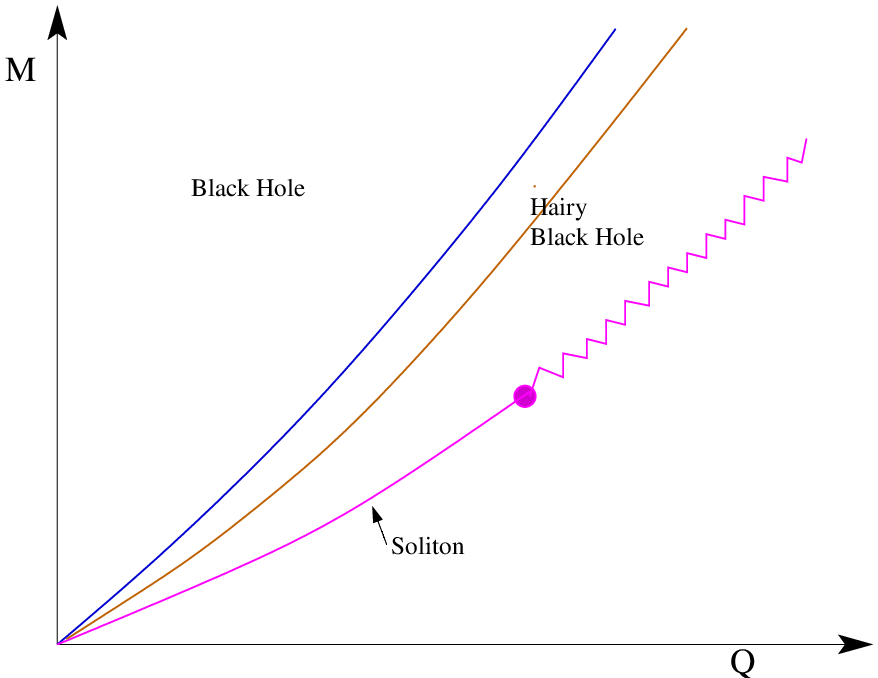
The main point of interest of the conjectured phase diagram of Fig. 3 is the lower edge of the diagram. As we have explained below, the hairy black hole phase is bounded from below by the solitonic solution at small mass and charge. The temperature of the hairy black hole also tends to infinity as we approach this line. On the other hand, it seems plausible that the solitonic solution goes singular past its ‘Chandrasekhar’ critical charge (the dot in Fig. 3). If this is indeed the case, it is of great interest to know the nature of the lower bound of Fig. 3 at higher values of the charge (the jagged line in Fig. 3). We get some information from studies of the system in the Poincare patch limit (see for instance [21, 22, 23]),so asymptotically large charges in Fig. 3. In this limit prior studies appear to suggest that the jagged line is the zero temperature limit of hairy black brane solution2424 24 It is interesting that the zero temperature limit of hairy black branes appears to depend qualitatively on the mass of the charged scalar field, and case is rather special. In the small black hole limit, on the other hand, we do not expect a qualitative dependence of our phase diagram on the mass of the scalar field. Indeed the leading order thermodynamics of hairy black holes in the Lagrangian (1) supplemented by a mass term for the scalar field can be easily obtained based on general non-interaction arguments (see 6.4) and it gives results that are qualitatively similar to the case. We thank A. Yarom for a discussion about this point.. If the phase diagram of Fig. 3 is indeed correct, it is natural to suppose that the jagged line everywhere represents the zero temperature limit of a hairy black hole. This suggests that the neighbourhood of the limiting soliton solution (the dot in Fig. 3) is extremely interesting. Hairy black holes on the solid lower line in the neighbourhood of this dot are at infinite temperature. On the other hand, points on the jagged line in the neighbourhood of this dot are at zero temperature. As we circle the dot from the solid to the jagged line we presumably pass through all temperatures in between. While all this is very speculative, would be very interesting to investigate it further.
Although all the analysis of this paper focussed on the concrete and especially simple context of charged black holes in the system (1), the basic physical picture of small hairy black holes as a linear combination of approximately non interacting pieces is based on very general considerations, should apply equally to the study of any bulk gravitational asymptotically AdS system that hosts RNAdS black holes which suffer from a superradiant instability. It should be straightforward to generalise the calculations of this paper to systems in which (1) is modified by the addition of a potential for the scalar field, and / or is studied in different dimensions. It may also be possible to generalise the constructions of this paper to superradiant instabilities in charged rotating black holes[24, 25].
As we have explained in section 2, at leading order in perturbation theory, small hairy black holes exist for , but do not exist when . The case lies on the edge, and is particularly interesting. The question of whether hairy black holes exist at this critical value is determined by a second rather than first order calculation. In the system under study in this paper, it turns out that hairy black holes do exist for . One way of understanding this statement goes as follows.
At any fixed value of the charge , hairy black holes exist if and only if where
(one may derive this result by comparing the mass of the soliton with the extremal RNAdS black hole at equal charge). It follows that small charge hairy black holes do exist at , but we have to go beyond leading order in perturbation theory to see this2525 25 On the other hand, the study of the near horizon BF bound in highly charged extremal black hole backgrounds (which are locally well-approximated by extremal black-branes) indicates that as , Note that the leading deviation from the black-brane result of is positive and in the large q limit continues to be monotonically decreasing. In other words, all available data is consistent with the conjecture that is a monotonically decreasing function that interpolates between and as ranges from 0 to . . Although we will not elaborate in detail in this paper, it turns out that the properties of small charged black holes at differ qualitatively from the properties of the same objects at larger . This observation is particularly relevant as it turns out that charged scalar fields are forced to sit at this critical value of charge in some natural supersymmetric bulk theories. We postpone the elaboration of these remarks and their consequences to future work.
A very interesting arena in which the ideas of this paper might find application is to the study of charged and rotating black holes in IIB theory on AdS. Small charged rotating black holes in IIB theory on AdS sometimes suffer from superradiant instabilities. It should be possible to apply the ideas of this to the study small black holes on AdS (we have started work in this direction). In this context one should, however, also keep in mind that small black holes in this system sometimes also suffer from Gregory Laflamme type instabilities[19] even when they are uncharged, a feature that complicates (but enriches) the study of this system.
Recall also that IIB supergravity on AdS hosts a 4 parameter set of one sixteenth BPS supersymmetric black hole solutions[26, 27, 28]. It is possible that there exist new BPS hairy black holes consisting of a non interacting mix of these SUSY black holes with a SUSY graviton condensate. It would be very interesting to investigate this further.
Acknowledgements
We would like to thank R. Gopakumar, S. Hartnoll, H. Liu, G. Mandal, K. Papadodimas, W. Song, A. Strominger, T. Takayanagi, S. Trivedi, S. Wadia and A. Yarom for useful discussions. We would also like to thank S.Hartnoll, G.Horowitz, K. Papadodimas, M.Rangamani, H.Reall , A.Strominger, S. Trivedi and A.Yarom for useful comments on a draft version of this manuscript. SM would like to thank IPMU for hospitality while this work was being completed. The work of SM was supported in part by a Swarnajayanti Fellowship. We must also acknowledge our debt to the steady and generous support of the people of India for research in basic science.
Appendix A Superradiant Instability of small black holes
In this section we analyse the dynamical stability of RNAdS black holes in AdS5 to superradiant emission in the presence of a massless charged minimally coupled scalar field. As we have explained in the introduction, we intuitively expect very small black hole to be unstable whenever . In this Appendix we verify this expectation by computing the frequency of the lowest quasi normal mode of the black hole in a perturbative expansion , the radius of the black hole. We find that the imaginary part of this frequency flips sign (from stable to unstable) as increases past , exactly as we expected on intuitive grounds.
We wish to compute the lowest quasi normal mode of (11) at small . By definition, quasi normal modes are regular at the future horizon, so it is useful to work in coordinates that are good at the future horizon. We choose to work in ingoing Eddington Finkelstein coordinate; in other words we replace the Schwarzschild time with the new time variable
where given by
| (64) |
In these new coordinates the background (11) takes the form
| (65) |
with
| (66) |
A linearised scalar fluctuation about this background takes the form
| (67) |
where
with being the background gauge field (66)
In the rest of this appendix we will solve (67) separately in a far field region, and a near field region . In the limit , of interest here, the solution may then be determined everwhere by matching the two solutions in their overlapping domain of validity. The matching procedure may be carried out systematically in a power series in , and turns out to determine the frequency of the quasi normal mode in a power series in . We carry out this procedure to order , the first order at which the quasi normal frequency develops an imaginary component. 2626 26 The fact that the quasi normal frequency first develops an imaginary piece at is simply related to the fact that the area - and so low frequency absorption cross section of a black hole in 5 dimensions - scales like .
A.1 Solution in near field region
When it is useful to work with the rescaled coordinate given by
Let the scalar fluctuation take the form
| (68) |
where
| (69) |
and
| (70) |
Note we have chosen to study the quasi normal mode with the frequency ; here we have used the physical expectation that the lowest quasinormal mode should reduce to the lowest normal mode in the limit . The energy of the lowest normal mode is .
It is a simple matter to solve (67) perturbatively in . Imposing the physical requirement of regularity at the horizon we find
| (71) |
where and are as yet undetermined integration constants (they will be determined below by matching). For brevity we have also presented the result assuming , a result that turns out to be forced on us by matching with the far field expansion below.
A.2 Solution in the far field region
In the outer region the fluctuation takes the form
| (72) |
where
| (73) |
Solving the equation of motion subject to the requirement of normalisability at large we find
| (74) |
and,
| (75) |
where once again we have presented the results only for . We have also plugged in the expression for and (this is forced on us by the matching condition below). Here besides imposing normalisability at infinity, we have also demanded that the coefficient of the leading normalisable piece is one.
A.3 Conditions for patch up
In order to complete our determination of the solution, we must now match the near and far field solutions. The logic for this matching procedure is exactly as described in subsection 3.3. Implementing this procedure we find
| (76) |
Also the quasi-normal frequency is determined to be
| (77) |
Once these matching conditions are imposed, the large expansion of the near field solution (with substituted by ) and the small expansion of the far field solution both share the common expansions
| (78) |
Equation (77) is the main result of this Appendix. Note that the imaginary part of turns positive as exceeds , demonstrating that RNAdS black holes with suffer from a super radiant instability.
Appendix B Results of the Low Order Perturbative Expansion of the Hairy Black Hole
In this Appendix we present explicit results for the perturbative expansion of the Hairy black hole solution at low orders in perturbation theory. See section 2 for explanation of the notation etc.
B.1 Near Field Expansion
| (79) |
| (80) |
| (81) |
| (82) |
where
| (83) |
B.2 Far Field Expansion
| (84) |
| (85) |
| (86) |
| (87) |
Appendix C The soliton at high orders in perturbation theory
C.1 Explicit Results to
As we have mentioned in section 5, the perturbation theory that generates the soliton solution as a function of is straightforward and hence may be automated on Mathematica. We have implemented this automation and used it to generate the ground state soliton solution to . For what its worth, we present the resultant explicit formulae for all thermodynamical quantities: the mass, the charge and the chemical potential to . Later in this appendix we will also speculate that our solution develops a singularity at the origin at a finite value of . To aid this discussion we also present formulas for and to the same order in .
C.2 Particular case
Of course, the formulae of the previous subsection are not immediately illuminating. In order to extract some (tentative) physical conclusions from those formulae, we specialise, in this section, to a particular value of , namely . At this specific value of we were able to coax Mathematica into producing results upto . We will not explicitly list our results, but use them to generate some plots that may carry qualitative lessons.
We are principally interested in the following question: does our solitonic solution develop a singularity (and so cease to exist) past a particular critical value of (or charge)? It would seem intuitively that this should be the case; no solitonic solution should exist at a mass greater than the ‘Chandrasekhar limit’ for this configuration.
Of course it is far from clear that perturbation theory can capture any phenomenon - particularly one as interesting as singularity formation - at finite values of . Nonetheless, in this subsection we will investigate the clues that we can glean from our perturbative analysis.


In Figs 4 and 5 we present a plot of at and at . We also present a plot of the scalar field at the origin as a function of . Note that is everywhere positive at while it goes negative near the origin at . Note also that the scalar field behaves quite smoothly at the origin at but shows a pronounced peak near the origin at .


We take these results to indicate that the actual solution develops a singularity at some value of between and . Let us use the vanishing of at the horizon as an estimator of the onset of this singularity. In Fig. 7 we plot as a function of . Note that this graph goes through the origin at .


In Figs 8 and 9 we plot the mass and charge of the solution as a function of . Note that these graphs do not show a pronounced peak near . We take this result to indicate that the mass and charge of the soliton are finite as we approach the singularity. All of the ‘conclusions’ of this subsection are at best suggestive. A more serious analysis of the perturbative expansions described in this appendix could plausibly yield more solid indications as to the existence (or otherwise) of a singularity in the solution (rather than simply in the perturbative expansion) at . Numerical solutions to the differential equations would also likely yield valuable insights here. We leave all such discussions to future work.
Appendix D Excited State Solitons
In this section, we will present explicit solution for the solitons obtained by populating the first and the second excited state.
D.1 The first excited state soliton
The solution obtained by populating the first excited state takes the form
| (88) |
Here C1 is a constant that will be determined by the regularity and normalisability conditions on at one higher order.
D.2 The second excited state soliton
The solution obtained by populating the second excited state is
| (89) |
Here again C1 is determined at one higher order. Finally the scalar field in this case is given by
| (90) |
Appendix E The First Excited Hairy Black Hole
In this Appendix we present the results of our construction of the first excited hairy black hole metric. We have written a Mathematica programme that allows us to generate the corresponding solution for the excited hairy black hole at any given value of . We use the same conventions as in appendixB.
E.1 Near Field Expansion
| (91) |
| (92) |
| (93) |
| (94) |
E.2 Far Field Solutions
| (95) |
| (96) |
| (97) |
| (98) |
In the above formulae and are constants which will only be determined by regularity and normalisability of the scalar field at one higher order.
Appendix F Thermodynamics in the Canonical Ensemble
In the following subsections, we will describe the canonical phase diagrams that result from a competition between small RNAdS black holes, small hairy black holes and small solitons. Everywhere in this section we completely ignore large black holes and large hairy black holes.
In the microcanonical ensemble this was logically justified; large black holes never have small mass and charge. However large black holes can (and do) have temperatures (and or chemical potentials) comparable to their small counterparts. Consequently the phase diagrams we will draw in this appendix do not, in general, represent the true thermo dynamical equilibrium of our system at finite temperature and chemical potential. The phase diagrams of this appendix should be regarded as formal; their purpose is to help us better understand the formal interrelationship between the phases constructed in this paper, ignoring all other phases that might exist in the system.
In this section we will study the interelationship between small black hole, soliton and excited black hole phases at fixed charge and temperature. We find it convenient to work with the rescaled inverse temperature variable
In this section we will assume that and are small. We also assume that and are of the same order, and present all formulae only to leading order in and .
F.1 RNAdS Black Hole
At any fixed charge, the temperature of a small RNAdS black hole is given, as a function of its chemical potential by
| (99) |

In Fig.10, we present a plot of versus . Note that
(the constraint follows directly from the requirement of positivity of the temperature in (99)). Note also that
| (100) |
This inequality is saturated at at .
Note that there exist two small black holes (with different values of ) for any given that obeys (100) The free energy is given as a function on and by
| (101) |


In Fig. 11 we present a plot of versus . Note that
and the minimum value occurs at (this is the same value of at which the temperature curve has a maximum). As is visually apparent from these graphs, the RNAdS black hole with the larger value of has lower free energy at any fixed and (see fig.12). In this appendix we will refer to this solution as the small RNAdS black hole. We will completely ignore the free energetically subdominant RNAdS black hole in the rest of this Appendix.
F.2 Soliton
Solitonic solutions exist at all values of and . At leading order the Free energy and chemical potential of the soliton are given by
| (102) |
Note that whenever
It follows that the soliton free energetically dominates that RNAdS black hole whenever this inequality is obeyed. At smaller values of , on the other hand, the RNAdS black hole free energetically dominates the soliton at large enough temperatures (but temperatures that are small enough to be allowed by (100), i.e. whenever
| (103) |
We will return to a more detailed comparison of phases below.
F.3 Hairy Black hole
Hairy black holes exist if and only if
| (104) |
In this regime their chemical potential, mass and free energy are given by
| (105) |
(where we have listed perturbative corrections, but will only use leading order results in what follows). Note that the difference between the free energy of a hairy black hole and the soliton is a positive number times , so that hairy black holes are free energetically always subdominant compared to the soliton.
It is also interesting to perform a comparison between RNAdS and hairy black holes. First notice that the existence ranges (104) and (100) overlap only when
Moreover hairy black holes only exist for . Within this range of hairy and RNAdS black holes in an overlapping region in the , plane. It turns out that RNAdS black holes always dominate over hairy black holes in these overlapping regions.
F.4 Plots of Phase Existence and Dominance
As we have explained above, the phase diagram of our system depends qualitatively on the value of . In particular, there are three special values of
Recall that RNAdS black holes are always stable - and no hairy black holes exist - for . In this regime the only phases of the system are the RNAdS black hole and the soliton. It turns out that the RNAdS black hole is free energetically dominant whenever it exists. The phase diagram is depicted in Fig.13 below.

RNAdS black holes exist only above the line drawn in Fig 13, and give the dominant phase when they exist. The soliton dominates the phase diagram elsewhere.
In the regime hairy black holes exist as a phase (below the topmost line in Fig. 14) but are never dominant. In this regime the RNAdS black holes exist above the bottom most line but free energetically dominate the soliton only in the region between the bottom most line and the intermediate line. The soliton is free energetically dominant elsewhere. The RNAdS black hole is free energetically dominant over the hairy black hole over their common region of existence.
In the regime the phase diagram (shown in Fig.15) is very similar to that in Fig.14, except that there is no intermediate region; the soliton is the thermodynamically dominant solution everywhere. Note that in this regime the RNAdS and hairy black hole solutions continue to exist as phases; the RNAdS black hole is free energetically dominant over the hairy black hole over this region of overlap (i.e., region B in 15).


We turn, finally to the range . Note that in this range . Recall that the chemical potential of a hairy black hole is equal to at leading order. It follows that the RNAdS black hole component of a hairy black hole, in this regime, has . In other words, in this regime, the RNAdS black hole that lies in the centre of a hairy black hole is of negative specific heat. In this regime, also, there is no overlap in the existence regimes of RNAdS black holes (100) and hairy black holes (104). At any given value of and we have at most two phases (soliton and black hole or soliton and hairy black hole) and the soliton is always the free energetically dominant phase. The phase diagram is displayed in Fig. 16

Appendix G Thermodynamics in the Grand Canonical Ensemble
In the following subsections, we will describe the grand canonical phase diagrams that result from a competition between small RNAdS black holes, small hairy black holes and small solitons. Everywhere in this section we completely ignore large black holes and large hairy black holes. Like our discussion on canonical ensemble given in the previous appendix, this is not entirely justified if we are interested in the actual phase diagram of the system. However, the formal diagrams which we present in this appendix are still helpful in contrasting the various phases constructed in this paper.
In this section we will study the thermodynamics of our system as a function of
G.1 RNAdS Black Holes
As we have seen above, small RNAdS black holes exist only for
Moreover these black holes also satisfy the inequality
This last inequality is automatically obeyed for parametrically small values of , of prime interest to us in this paper, and so will play no important role in the analysis below. Whenever these inequalities are satisfied, we have a unique small black hole.
The various important thermodynamical quantities of small RNAdS black holes, in the grand canonical ensemble, are given by
| (106) |
| (107) |
G.2 Soliton
The soliton exists for all temperatures but for . Its thermodynamical quantities are given by
| (108) |
It is easy to verify that the solitonic solution always has lower grand free energy (it is negative at leading order) than the RNAdS black hole (the free energy is positive at leading order ) within the validity of perturbation theory. Consequently the system undergoes a first order phase transition from the RNAdS black hole to the solitonic phase as is raised above
G.3 Hairy Black hole
Hairy black holes exist whenever
| (109) |
Their thermodynamical quantities are given by
| (110) |
It is easily verified that (within perturbation theory) hairy black holes are free energetically subdominant compared to solitons in their common domain of existence. On the other hand, it may be checked that they are free energetically dominant compared to RNAdS black holes, where the solutions coexist.
G.4 Phase Diagrams
The phase diagram of our system is very simple when . Hairy black holes don’t exist. The two phases that do exist - RNAdS black holes and the soliton - never coexist at the same and . The RNAdS black hole dominates when it exists; the soliton dominates when it exists. The phase diagram is sketched in Fig.17 below.


The phase diagram is more interesting when . As we have mentioned above, the system undergoes a first order phase transition from the black hole to the solitonic phase as is raised above . The hairy black hole phase is always subdominant compared to the soliton, but free energetically dominates the black hole when both exist. The phase diagram is depicted in Fig. 18 below. Note that the black hole and hairy black holes phases are identical, where the hairy black hole is first created. In the absence of the solitonic solution, consequently, our system would have undergone a second order transition from the RNAdS black hole to the hairy black hole phase upon raising .
Appendix H Notation
H.1 Basic Setup
Throughout this paper, we work in asymptotically (global) AdS5 spacetimes with a bulk metric , a bulk charged scalar field and a bulk gauge field with a Lagrangian
| (111) |
where is the Newtons’s constant and the radius of AdS5 is set to unity. This implies that the bulk cosmological constant is taken to be .
The radial co-ordinate of AdS5 is denoted by with the boundary of AdS5 being at . For solutions with the horizon, the outer horizon is taken to be at . The Schwarzschild-like temporal co-ordinate is denoted by . Sometimes, we find it convenient to work with rescaled co-ordinates and , especially in the near-field expansion at small radius (). In Appendix A, we shift to Eddington-Finkelstein like co-ordinates, with an Eddington-Finkelstein(EF) time co-ordinate denoted by .
Since throughout this paper we work with spherically symmetric solutions, we will leave the co-ordinates parametrising S3 implicit. Mostly, we work in a gauge where the bulk fields take a form
| (112) |
In Appendix A, we work with the EF co-ordinate metric for a small charged black hole (see below).
The charge of the scalar field is denoted by and its mass by . We take for most of the paper except in section 6.4 . By the standard rules of AdS/CFT, the dual boundary operator has a scaling dimension
This is also the energy of the lowest mode in vacuum AdS5. For the case , . The other spherically symmetric modes of (dual to the descendants ) have an energy
For the case , . The covariant derivative acting on is denoted by . The symbol is used to denote the covariant Laplacian.
H.2 Thermodynamic quantities
We now turn to notations involving thermodynamic quantities. First, we omit a factor of from all our extensive quantities in order to simplify our expressions. With this understanding, we will denote the ADM mass by , the charge of a solution by and its entropy by . We often find it convenient to work with a rescaled mass and a rescaled charge which are related to the actual mass and charge via the relations
| (113) |
We use to denote Helmholtz free-energy appropriate to the canonical ensemble and to denote the grand potential appropriate to the grand-canonical ensemble. Coming to the intensive variables represents the chemical potential and represents the temperature both of which are defined by the first law
We sometimes find it convenient to work with the ‘rationalised’ inverse temperature and the chemical potential excess over the super-radiant bound .
H.3 Double expansions
Quantities in this paper are often expressed as double expansions about two parameters - first is the parameter which is the amplitude of the leading normalisable mode in . Under AdS/CFT, roughly , the boundary expectation value of , the operator dual to . The second parameter is the outer horizon radius of the small charged blackhole at the core of the hairy blackhole. Further, our solutions are often expressed in terms of a matched asymptotic expansion with a near-field expansion at small radius () and a far field expansion far away from the horizon () matched at their common domain of validity. We use the superscripts and to denote these two expansions respectively. Many formulae in this paper involve the coefficients in this expansion which are defined via
| (114) |
In a similar vein, one can define an expansion of the covariant Laplacian
Further, the boundary value of the gauge field or the chemical potential has the double expansion
References
- [1] S. S. Gubser, Breaking an Abelian gauge symmetry near a black hole horizon, Phys. Rev. D78 (2008) 065034, [arXiv:0801.2977].
- [2] S. Sachdev, Condensed matter and AdS/CFT, arXiv:1002.2947.
- [3] G. T. Horowitz, Introduction to Holographic Superconductors, arXiv:1002.1722.
- [4] S. A. Hartnoll, Quantum Critical Dynamics from Black Holes, arXiv:0909.3553.
- [5] S. A. Hartnoll, Lectures on holographic methods for condensed matter physics, Class. Quant. Grav. 26 (2009) 224002, [arXiv:0903.3246].
- [6] C. P. Herzog, Lectures on Holographic Superfluidity and Superconductivity, J. Phys. A42 (2009) 343001, [arXiv:0904.1975].
- [7] P. Basu, J. He, A. Mukherjee, and H.-H. Shieh, Superconductivity from D3/D7: Holographic Pion Superfluid, JHEP 11 (2009) 070, [arXiv:0810.3970].
- [8] C. P. Herzog and S. S. Pufu, The Second Sound of SU(2), JHEP 04 (2009) 126, [arXiv:0902.0409].
- [9] R. Gregory, S. Kanno, and J. Soda, Holographic Superconductors with Higher Curvature Corrections, JHEP 10 (2009) 010, [arXiv:0907.3203].
- [10] J. Sonner, A Rotating Holographic Superconductor, Phys. Rev. D80 (2009) 084031, [arXiv:0903.0627].
- [11] J. D. Bekenstein, Extraction of energy and charge from a black hole, Phys. Rev. D7 (1973) 949–953.
- [12] W. H. Press and S. A. Teukolsky, Floating Orbits, Superradiant Scattering and the Black-hole Bomb, Nature 238 (July, 1972) 211–212.
- [13] T. Nishioka, S. Ryu, and T. Takayanagi, Holographic Superconductor/Insulator Transition at Zero Temperature, arXiv:0911.0962.
- [14] D. Kastor and J. H. Traschen, Horizons inside classical lumps, Phys. Rev. D46 (1992) 5399–5403, [hep-th/9207070].
- [15] F. E. Schunck and E. W. Mielke, General relativistic boson stars, Class. Quant. Grav. 20 (2003) R301–R356, [arXiv:0801.0307].
- [16] D. Astefanesei and E. Radu, Boson stars with negative cosmological constant, Nucl. Phys. B665 (2003) 594–622, [gr-qc/0309131].
- [17] R. M. Wald, On the instability of the n=1 Einstein Yang-Mills black holes and mathematically related systems, J. Math. Phys. 33 (1992) 248–255.
- [18] M. D. Seifert and R. M. Wald, A general variational principle for spherically symmetric perturbations in diffeomorphism covariant theories, Phys. Rev. D75 (2007) 084029, [gr-qc/0612121].
- [19] V. E. Hubeny and M. Rangamani, Unstable horizons, JHEP 05 (2002) 027, [hep-th/0202189].
- [20] K. Maeda, J.-i. Koga, and S. Fujii, The final fate of instability of Reissner-Nordstróm- anti-de Sitter black holes by charged complex scalar fields, arXiv:1003.2689.
- [21] S. S. Gubser and F. D. Rocha, The gravity dual to a quantum critical point with spontaneous symmetry breaking, Phys. Rev. Lett. 102 (2009) 061601, [arXiv:0807.1737].
- [22] S. S. Gubser and A. Nellore, Ground states of holographic superconductors, Phys. Rev. D80 (2009) 105007, [arXiv:0908.1972].
- [23] G. T. Horowitz and M. M. Roberts, Zero Temperature Limit of Holographic Superconductors, JHEP 11 (2009) 015, [arXiv:0908.3677].
- [24] H. K. Kunduri, J. Lucietti, and H. S. Reall, Gravitational perturbations of higher dimensional rotating black holes: Tensor Perturbations, Phys. Rev. D74 (2006) 084021, [hep-th/0606076].
- [25] V. Cardoso, O. J. C. Dias, and S. Yoshida, Classical instability of Kerr-AdS black holes and the issue of final state, Phys. Rev. D74 (2006) 044008, [hep-th/0607162].
- [26] J. P. Gauntlett, J. B. Gutowski, C. M. Hull, S. Pakis, and H. S. Reall, All supersymmetric solutions of minimal supergravity in five dimensions, Class. Quant. Grav. 20 (2003) 4587–4634, [hep-th/0209114].
- [27] J. B. Gutowski and H. S. Reall, Supersymmetric AdS(5) black holes, JHEP 02 (2004) 006, [hep-th/0401042].
- [28] J. B. Gutowski and H. S. Reall, General supersymmetric AdS(5) black holes, JHEP 04 (2004) 048, [hep-th/0401129].
- [29] H. Lin, O. Lunin, and J. M. Maldacena, Bubbling AdS space and 1/2 BPS geometries, JHEP 10 (2004) 025, [hep-th/0409174].
*