Many-body physics from a quantum information perspective

R. Augusiak F. M. Cucchietti and M. Lewenstein Affiliation: Remigiusz Augusiak Affiliation: ICFO–Institut de Ciències Fotòniques, Mediterranean Technology Park, 08860 Castelldefels (Barcelona), Spain, Affiliation: ICFO–Institut de Ciències Fotòniques, Mediterranean Technology Park, 08860 Castelldefels (Barcelona), Spain, ICREA–Institució Catalana de Recerca i Estudis Avançats, Lluis Companys 23, 08010 Barcelona, Spain E-mail: maciej.lewenstein@icfo.es

Abstract

The quantum information approach to many-body physics has been very successful in giving new insights and novel numerical methods. In these lecture notes we take a vertical view of the subject, starting from general concepts and at each step delving into applications or consequences of a particular topic. We first review some general quantum information concepts like entanglement and entanglement measures, which leads us to entanglement area laws. We then continue with one of the most famous examples of area-law abiding states: matrix product states, and tensor product states in general. Of these, we choose one example (classical superposition states) to introduce recent developments on a novel quantum many-body approach: quantum kinetic Ising models. We conclude with a brief outlook of the field.

1 Introduction

There has been an explosion of interest in the interface between quantum information (QI) and many-body systems, in particular in the fields of condensed matter and ultracold atomic gases. Remarkable examples are Ref. [1], which proposed using ultracold atomic gases in optical lattices for QI (and stimulated interest in distributed quantum information processing), and Refs. [2, 3, 4], who discussed the first connections between entanglement and quantum phase transitions (QPT). Overall, the confluence of ideas has opened fundamentally deep questions about QPT’s, as well as practical questions about how to use QI ideas in numerical simulations of many-body quantum systems. Here, we will (partially) review these two major themes. We will first introduce some basic notions and tools of quantum information theory, focusing on entanglement and entanglement measures. We shall then discuss area laws, i.e. laws that characterize correlations and entanglement in physically relevant many-body states, and allow to make general statements about computational complexity of the corresponding Hamiltonians. Afterwards, we will explore the concept of matrix product states (MPS) and their generalizations (projected entangled pairs states, PEPS, and tensor networks states). These states provide not only a very useful ansatz for numerical applications, but also a powerful tool to understand the role of entanglement in the quantum many-body theory. We will review one particular example of a state with a straightforward MPS representation: the classical superposition state. The introduction of its parent Hamiltonian will lead us to the final subject of these lectures: quantum kinetic Ising models — an analytically solvable generalization of the popular classical many-body model described by a master equation.

2 Aspects of Quantum Information

Quantum theory contains elements that are radically different from our everyday (“classical”) description of Nature: a most important example are the quantum correlations present in quantum formalism. Classically, complete knowledge of a system implies that the sum of the information of its subsystems makes up the total information for the whole system. In the quantum world, this is no longer true: there exist states of composite systems about which we have complete information, but we know nothing about its subsystems. We may even reach paradoxical conclusions if we apply a classical description to such “entangled” states—whose concept can be traced back to 1932 in manuscripts of E. Schrödinger.

What we have just realized during the last two decades is that these fundamentally nonclassical states (from hereon “entangled states”) can provide us with more than just paradoxes: They may be used to perform tasks that cannot be achieved with classical states. As landmarks of this transformation in our view of such nonclassical states, we mention the spectacular discoveries of (entanglement-based) quantum cryptography [5], quantum dense coding [6], and quantum teleportation [7]. Even though our knowledge of entanglement is still far from complete, significant progress has been made in the recent years and very active research is currently underway (for a recent and very complete review see [8]).

In the next section, we will focus on bipartite composite systems. We will define formally what entangled states are, present some important criteria to discriminate entangled states from separable ones, and show how they can be classified according to their capability to perform some precisely defined tasks. However, before going into details, let us introduce the notation. In what follows we will be mostly concerned with bipartite scenarios, in which traditionally the main roles are played by two parties called Alice and Bob. Let $\mathcal{H}_{A}$ denote the Hilbert space of Alice’s physical system, and $\mathcal{H}_{B}$ that of Bob’s. Our considerations will be restricted to finite-dimensional Hilbert spaces, so we can set $\mathcal{H}_{A}=\mathbb{C}^{d_{A}}$ and $\mathcal{H}_{B}=\mathbb{C}^{d_{B}}$ . Thus, the joint physical system of Alice and Bob is described by the tensor product Hilbert space $\mathcal{H}_{AB}=\mathcal{H}_{A}\otimes\mathcal{H}_{B}=\mathbb{C}^{d_{A}}\otimes\mathbb{C}^{d_{B}}$ . Finally, $\mathcal{B}(\mathcal{H})$ will denote the set of bounded linear operators from the Hilbert space $\mathcal{H}$ to $\mathcal{H}$ .

2.1 Bipartite pure states: Schmidt decomposition

We start our study with pure states, for which the concepts are simpler. Pure states are either separable or entangled states according to the following definition:

Definition 1

Consider a pure state $|\psi_{AB}\rangle$ from $\mathcal{H}_{A}\otimes\mathcal{H}_{B}$ . It is called separable if there exist pure states $|\psi_{A}\rangle\in\mathcal{H}_{A}$ and $|\psi_{B}\rangle\in\mathcal{H}_{B}$ such that $|\psi_{AB}\rangle=|\psi_{A}\rangle\otimes|\psi_{B}\rangle$ . Otherwise we say that $|\psi_{AB}\rangle$ is entangled.

The most famous examples of entangled states in $\mathcal{H}_{AB}$ are the maximally entangled states, given by

|\psi_{+}^{(d)}\rangle=\frac{1}{\sqrt{d}}\sum_{i=0}^{d-1}|i\rangle_{A}\otimes|i\rangle_{B}\qquad(d=\min\{d_{A},d_{B}\}),

(1)

where the vectors $\{|i\rangle_{A}\}$ and $\{|i\rangle_{B}\}$ form bases (in particular they can be the standard ones) in $\mathcal{H}_{A}$ and $\mathcal{H}_{B}$ , respectively. In what follows, we also use $P_{+}^{(d)}$ to denote the projector onto $|\psi_{+}^{(d)}\rangle$ . The reason why this state is called maximally entangled will become clear when we introduce entanglement measures.

In pure states, the separability problem — the task of judging if a given quantum state is separable — is easy to handle using the concept of Schmidt decomposition:

Theorem 2.1

Let $|\psi_{AB}\rangle\in\mathcal{H}_{AB}=\mathbb{C}^{d_{A}}\otimes\mathbb{C}^{d_{B}}$ with $d_{A}\leq d_{B}$ . Then $|\psi_{AB}\rangle$ can be written as a Schmidt decomposition

|\psi_{AB}\rangle=\sum_{i=1}^{r}\lambda_{i}|e_{i}\rangle\otimes|f_{i}\rangle,

(2)

where $|e_{i}\rangle$ and $|f_{i}\rangle$ form a part of an orthonormal basis in $\mathcal{H}_{A}$ and $\mathcal{H}_{B}$ , respectively, $\lambda_{i}>0$ , $\sum_{i=1}^{r}\lambda_{i}^{2}=1$ , and $r\leq d_{A}$ .

Proof

A generic pure bipartite state $|\psi_{AB}\rangle$ can be written in the standard basis of $\mathcal{H}_{A}\otimes\mathcal{H}_{B}$ as $|\psi_{AB}\rangle=\sum_{i=0}\sum_{j=0}\alpha_{ij}|i\rangle\otimes|j\rangle$ , where, in general, the coefficients $\alpha_{ij}$ form a $d_{A}\times d_{B}$ matrix $\Lambda$ obeying $\mathrm{tr}(\Lambda^{\dagger}\Lambda)=1$ . Using singular-value decomposition, we can write $\Lambda=VD_{\Lambda}W^{\dagger}$ , where $V$ and $W$ are unitary ( $V^{\dagger}V=W^{\dagger}W=\mathbbm{1}_{A}$ ) and $D_{\Lambda}$ is diagonal matrix consisting of the eigenvalues $\lambda_{i}$ of $|\Lambda|=\sqrt{\Lambda^{\dagger}\Lambda}$ . Using this we rewrite $|\psi_{AB}\rangle$ as

|\psi_{AB}\rangle=\sum_{i=0}^{d_{A}-1}\sum_{j=0}^{d_{B}-1}\sum_{k=1}^{r}V_{ik}\lambda_{k}U_{jk}^{*}|i\rangle|j\rangle,

(3)

where $r\leq d_{A}\leq d_{B}$ denotes the rank of $\Lambda$ . By reshuffling terms, and defining $|e_{k}\rangle=\sum_{i=0}^{d_{A}-1}V_{ik}|i\rangle$ and $|f_{k}\rangle=\sum_{j=0}^{d_{B}-1}U^{*}_{jk}|j\rangle$ we get the desired form [Eq. (2)]. To complete the proof, we notice that due to the unitarity of $V$ and $W$ , vectors $|e_{i}\rangle$ and $|f_{i}\rangle$ satisfy $\langle e_{i}|e_{j}\rangle=\langle f_{i}|f_{j}\rangle=\delta_{ij}$ , and constitute bases of $\mathcal{H}_{A}$ and $\mathcal{H}_{B}$ , respectively. In fact, $\{\lambda_{i}^{2},|e_{i}\rangle\}$ and $\{\lambda_{i}^{2},|f_{i}\rangle\}$ are eigensystems of the first and second subsystem of $|\psi_{AB}\rangle$ . Moreover, since $\mathrm{tr}(\Lambda^{\dagger}\Lambda)=1$ it holds that $\sum_{i}\lambda^{2}_{i}=1$ . $\blacksquare$

The numbers $\lambda_{i}>0$ $(i=1,\ldots,r)$ are called the Schmidt coefficients, and $r$ the Schmidt rank of $|\psi_{AB}\rangle$ . One can also notice that $\{\lambda_{i}^{2},|e_{i}\rangle\}$ and $\{\lambda_{i}^{2},|f_{i}\rangle\}$ are eigensystems of the first and second subsystem of $|\psi_{AB}\rangle$ , and that the Schmidt rank $r$ denotes the rank of both subsystems. Then, comparison with definition 2.1 shows that bipartite separable states are those with Schmidt rank one. Thus, to check if a given pure state is separable, it suffices to check the rank $r$ of one of its subsystems. If $r=1$ (the corresponding subsystem is in a pure state) then $|\psi_{AB}\rangle$ is separable; otherwise it is entangled. Notice that the maximally entangled state (1) is already written in the form (2), with $r=d$ and all the Schmidt coefficients equal to $1/\sqrt{d}$ .

2.2 Bipartite mixed states: Separable and entangled states

The easy-to-handle separability problem in pure states complicates considerably in the case of mixed states. In order to understand the distinction between separable and entangled mixed states — first formalized by Werner in 1989 [9] — let us consider the following state preparation procedure. Suppose that Alice and Bob are in distant locations and can produce and manipulate any physical system in their laboratories. Moreover, they can communicate using a classical channel (for instance a phone line). However, they do not have access to quantum communication channels, i.e. they are not allowed to exchange quantum states. These two capabilities, i.e. local operations (LO) and classical communication (CC), are frequently referred to as LOCC.

Suppose now that in each round of the preparation scheme, Alice generates with probability $p_{i}$ a random integer $i$ $(i=1,\ldots,K)$ , which she sends to Bob. Depending on this number, in each round Alice prepares a pure state $|e_{i}\rangle$ , and Bob a state $|f_{i}\rangle$ . After many rounds, the result of this preparation scheme is of the form

\displaystyle\varrho_{AB}=\sum_{i=1}^{K}p_{i}|e_{i}\rangle\!\langle e_{i}|\otimes|f_{i}\rangle\!\langle f_{i}|,

(4)

which is the most general one that can be prepared by Alice and Bob by means of LOCC. In this way we arrive at the formal definition of separability in the general case of mixed states.

Definition 2

We say that a mixed state $\varrho_{AB}$ acting on $\mathcal{H}_{AB}$ is separable if and only if it can be represented as a convex combination of the product of projectors on local states as in Eq. (4). Otherwise, the mixed state is said to be entangled.

The number of pure separable states $K$ necessary to decompose any separable state according to Eq. (4) is limited by the Caratheodory theorem as $K\leq(d_{A}d_{B})^{2}$ (see Refs. [10, 8]). No better bound is known in general, however, for two-qubit and qubit-qutrit systems it was shown that $K\leq 4$ [11] and $K\leq 6$ [12], respectively.

By definition, entangled states cannot be prepared locally by two parties even after communicating over a classical channel. To prepare entangled states, the physical systems must be brought together to interact¹¹ 1 Due to entanglement swapping [13], one must suitably enlarge the notion of preparation of entangled states. So, an entangled state between two particles can be prepared if and only if either the two particles (call them A and B) themselves come together to interact at a time in the past, or two other particles (call them C and D) do the same, with C having interacted beforehand with A and D with B.. Mathematically, a nonlocal unitary operator²² 2 A unitary operator on $\mathcal{H}_{A}\otimes\mathcal{H}_{B}$ is said to be “nonlocal” if it is not of the form $U_{A}\otimes U_{B}$ , where $U_{A}$ is a unitary operator acting on $\mathcal{H}_{A}$ and $U_{B}$ acts on $\mathcal{H}_{B}$ . must necessarily act on the physical system described by $\mathcal{H}_{A}\otimes\mathcal{H}_{B}$ to produce an entangled state from an initial separable state.

The question whether a given bipartite state is separable or not turns out to be quite complicated. Although the general answer to the separability problem still eludes us, there has been significant progress in recent years, and we will review some such directions in the following paragraphs.

2.3 Entanglement criteria

An operational necessary and sufficient criterion for detecting entanglement still does not exist. However, over the years the whole variety of criteria allowing for detection of entanglement has been worked out. Below we review some of the most important ones, while for others the reader is referred to Ref. [14]. Note that, even if we do not have necessary and sufficient separability criteria, there are numerical checks of separability: semidefinite programming was used to show that separability can be tested in a finite number of steps, although this number can become too large for big systems [15, 16]. In general —without a restriction on dimensions— the separability problem belongs to the NP-hard class of computational complexity [17].

2.4 Partial Transposition

Let us start with an easy–to–apply necessary criterion based on the transposition map recognized by Choi [18] and then independently formulated directly in the separability context by Peres [19].

Let $\varrho_{AB}$ be a state on the product Hilbert space ${\cal H}_{AB}$ , and $T:\mathcal{B}(\mathbb{C}^{d})\to\mathcal{B}(\mathbb{C}^{d})$ a transposition map with respect to some real basis $\{|i\rangle\}$ in $\mathbb{C}^{d}$ , defined through $T(X)\equiv X^{T}=\sum_{i,j}x_{ij}|j\rangle\!\langle i|$ for any $X=\sum_{i,j}x_{ij}|i\rangle\!\langle j|$ from $\mathcal{B}(\mathbb{C}^{d})$ . Let us now consider an extended map $T\otimes I_{B}$ called hereafter partial transposition, where $I_{B}$ is the identity map acting on the second subsystem. When applied to $\varrho_{AB}$ , the map $T\otimes I_{B}$ transposes the first subsystem leaving the second one untouched. More formally, writing $\varrho_{AB}$ as

\varrho_{AB}=\sum_{i,j=0}^{d_{A}-1}\sum_{\mu,\nu=0}^{d_{B}-1}\varrho_{ij}^{\mu\nu}|i\rangle\!\langle j|\otimes|\mu\rangle\!\langle\nu|,

(5)

where $\{|i\rangle\}$ and $\{|\mu\rangle\}$ are real bases in Alice and Bob Hilbert spaces, respectively, we have

(T\otimes I_{B})(\varrho_{AB})\equiv\varrho_{AB}^{T_{A}}=\sum_{i,j=0}^{d_{A}-1}\sum_{\mu,\nu=0}^{d_{B}-1}\varrho_{ij}^{\mu\nu}|j\rangle\!\langle i|\otimes|\mu\rangle\!\langle\nu|.

(6)

Similarly, one may define partial transposition with respect to the Bob’s subsystem (denoted by $\varrho_{AB}^{T_{B}}$ ). Although the partial transposition of $\varrho_{AB}$ depends upon the choice of the basis in which $\varrho_{AB}$ is written, its eigenvalues are basis independent. The applicability of the transposition map in the separability problem can be formalized by the following statement [19].

Theorem 2.2

If a state $\rho_{AB}$ is separable, then $\rho_{AB}^{T_{A}}\ \geq\ 0$ and $\rho_{AB}^{T_{B}}\ \geq\ 0$ .

Proof

Since $\varrho_{AB}$ is separable, according to definition 2 it has the form (4). Then, performing the partial transposition with respect to the first subsystem, we have

\displaystyle\rho_{AB}^{T_{A}}=\sum_{i=1}^{K}\ p_{i}\left(|e_{i}\rangle\!\langle e_{i}|\right)^{T_{A}}\otimes|f_{i}\rangle\!\langle f_{i}|=\sum_{i=1}^{K}\ p_{i}|e_{i}^{*}\rangle\!\langle e_{i}^{*}|\otimes|f_{i}\rangle\!\langle f_{i}|.

(7)

In the second step we used that $A^{\dagger}=\left(A^{*}\right)^{T}$ for all $A$ . The above shows that $\rho_{AB}^{T_{A}}$ is a proper (and also separable) density matrix implying that $\rho_{AB}^{T_{A}}\geq 0$ . The same reasoning leads to the conclusion that $\rho_{AB}^{T_{B}}\geq 0$ , finishing the proof. $\blacksquare$

Due to the identity $\varrho_{AB}^{T_{B}}=(\varrho_{AB}^{T_{A}})^{T}$ , and the fact that global transposition does not change eigenvalues, partial transpositions with respect to the $A$ and $B$ subsystems are equivalent from the point of view of the separability problem.

In conclusion, we have a simple criterion (partial transposition criterion) for detecting entanglement. More precisely, if the spectrum of one of the partial transpositions of $\varrho_{AB}$ contains at least one negative eigenvalue then $\varrho_{AB}$ is entangled. As an example, let us apply the criterion to pure entangled states. If $|\psi_{AB}\rangle$ is entangled, it can be written as (2) with $r>1$ . Then, the eigenvalues of $|\psi_{AB}\rangle\!\langle\psi_{AB}|^{T_{A}}$ will be $\lambda_{i}^{2}$ $(i=1,\ldots,r)$ and $\pm\lambda_{i}\lambda_{j}$ $(i\neq j\;i,j=1,\ldots,r)$ . So, an entangled $|\psi_{AB}\rangle$ of Schmidt rank $r>1$ has partial transposition with $r(r-1)/2$ negative eigenvalues violating the criterion stated in theorem 2.2.

The partial transposition criterion allows to detect in a straightforward manner all entangled states that have non–positive partial transposition (hereafter called NPT states). However, even if this is a large class of states, it turns out that —as pointed out in Refs. [10, 20]--- there exist entangled states with positive partial transposition (called PPT states) (cf. Fig. 2). Moreover, the set of PPT entangled states does not have measure zero [21]. It is, therefore, important to have further independent criteria that identify entangled PPT states. Remarkably, PPT entangled states are the only known examples of bound entangled states, i.e., states from which one cannot distill entanglement by means of LOCC, even if the parties have an access to an unlimited number of copies of the state [20, 8]. The conjecture that there exist NPT “bound entangled” states is one of the most challenging open problems in quantum information theory [22, 23]. Note also that both separable as well as PPT states form convex sets.

Theorem 2.2 is a necessary condition of separability in any arbitrary dimension. However, for some special cases, the partial transposition criterion is both a necessary and sufficient condition for separability [24]:

Theorem 2.3

A state $\varrho_{AB}$ acting on $\mathbb{C}^{2}\otimes\mathbb{C}^{2}$ or $\mathbb{C}^{2}\otimes\mathbb{C}^{3}$ is separable if and only if $\varrho_{AB}^{T_{A}}\ \geq\ 0$ .

We will prove this theorem later. Also, we will see that Theorem 2.2 is true for a whole class of maps (of which the transposition map is only a particular example), which also provide a sufficient criterion for separability. Before this, let us discuss the dual characterization of separability via entanglement witnesses.

2.5 Entanglement Witnesses from the Hahn-Banach theorem

Central to the concept of entanglement witnesses is the corollary from the Hahn--Banach theorem (or Hahn--Banach separation theorem), which we will present here limited to our needs and without proof (which the reader can find e.g. in Ref. [25]).

Theorem 2.4

Let $S$ be a convex compact set in a finite–dimensional Banach space. Let $\rho$ be a point in this space, however, outside of the set $S$ ( $\rho\not\in S$ ). Then there exists a hyperplane³³ 3 A hyperplane is a linear subspace with dimension smaller by one than the dimension of the space itself. that separates $\rho$ from $S$ .

Figure 1: Schematic picture of the Hahn-Banach theorem. The (unique) unit vector orthonormal to the hyperplane can be used to define right and left with respect to the hyperplane by using the sign of the scalar product.

The statement of the theorem is illustrated in figure 1. In order to apply it to our problem let $S$ denote now the set of all separable states acting on $\mathcal{H}_{A}\otimes\mathcal{H}_{B}$ . This is a convex compact subset of the Banach space of all the linear operators $\mathcal{B}(\mathcal{H}_{A}\otimes\mathcal{H}_{B})$ . The theorem implies that for any entangled state $\varrho_{AB}$ there exists a hyperplane separating it from $S$ .

Let us introduce a coordinate system located within the hyperplane (along with an orthogonal vector $W$ chosen so that it points towards $S$ ). Then, every state $\varrho_{AB}$ can be characterized by its ‘‘distance” from the plane, here represented by the Hilbert--Schmidt scalar product⁴⁴ 4 Let $\mathcal{H}$ be some Hilbert space. Then the set $\mathcal{B}(\mathcal{H})$ of linear bounded operators acting on $\mathcal{H}$ is also a Hilbert space with the Hilbert-Schmidt scalar product $\langle A|B\rangle=\mathrm{tr}(A^{\dagger}B)$ ( $A,B\in\mathcal{B}(\mathcal{H})$ ). . According to our choice of the coordinate system (see Fig. 1), for any such hyperplane $W$ every separable state has a positive “distance”, while there are some entangled states with a negative “distance”. More formally, theorem (2.4) implies the following seminal result [24].

Theorem 2.5

Let $\varrho_{AB}$ be some entangled state acting on $\mathcal{H}_{AB}$ . Then there exists a Hermitian operator $W\in\mathcal{B}(\mathcal{H}_{A}\otimes\mathcal{H}_{B})$ such that $\mathrm{tr}(\varrho_{AB}W)<0$ and $\mathrm{tr}(\sigma_{AB}W)\geq 0$ for all separable $\sigma_{AB}\in\mathcal{B}(\mathcal{H}_{A}\otimes\mathcal{H}_{B})$ .

It is then clear that all the operators $W$ representing such separating hyperplanes deserve special attention as they are natural candidates for entanglement detectors. That is, given some Hermitian $W$ , if $\mathrm{tr}(W\varrho_{AB})<0$ and simultaneously $\mathrm{tr}(W\sigma_{AB})\geq 0$ for all separable $\sigma_{AB}$ , we know that $\varrho_{AB}$ is entangled. One is then tempted to introduce the following definition [26].

Definition 3

We call the Hermitian operator $W$ an entanglement witness if $\mathrm{tr}(W\sigma_{AB})\geq 0$ for all separable $\sigma_{AB}$ and there exists an entangled state $\varrho_{AB}$ such that $\mathrm{tr}(W\varrho_{AB})<0$ .

Example 1

Let us discuss how to construct entanglement witnesses for all NPT states. If $\varrho_{AB}$ is NPT then its partial transposition has at least one negative eigenvalue. Let $|\psi_{i}\rangle$ denote the eigenstates of $\varrho^{T_{B}}_{AB}$ corresponding to its negative eigenvalues $\lambda_{i}<0$ . Then the Hermitian operator $W_{i}=|\psi_{i}\rangle\!\langle\psi_{i}|^{T_{B}}$ has negative mean value on $\varrho_{AB}$ , i.e., $\mathrm{tr}(\varrho_{AB}|\psi_{i}\rangle\!\langle\psi_{i}|^{T_{B}})=\mathrm{tr}(\varrho_{AB}^{T_{B}}|\psi_{i}\rangle\!\langle\psi_{i}|)=\lambda_{i}<0$ . Simultaneously, using the identity $\mathrm{tr}(AB^{T})=\mathrm{tr}(A^{T}B)$ obeyed by any pair of matrices $A$ and $B$ , it is straightforward to verify that $\mathrm{tr}(W_{i}\sigma_{AB})\geq 0$ for all $i$ and separable $\sigma_{AB}$ . One notices also that any convex combination of $W_{i}$ and in particular $\varrho_{AB}^{T_{B}}$ itself are also entanglement witnesses.

Let us comment shortly on the properties of entanglement witnesses. First, it is clear that they have negative eigenvalues, as otherwise their mean value on all entangled states would be positive. Second, since entanglement witnesses are Hermitian, they can be treated as physical observables — which means that separability criteria based on entanglement witnesses are interesting from the experimental point of view. Third, even if conceptually easy, entanglement witnesses depend on states in the sense that there exist entangled states that are only detected by different witnesses. Thus, in principle, the knowledge of all entanglement witnesses is necessary to detect all entangled states.

2.6 Positive maps and the entanglement problem

Transposition is not the only map that can be used to deal with the separability problem. It is rather clear that the statement of theorem 2.2 remains true if, instead of the transposition map, one uses any map that when applied to a positive operator gives again a positive operator (a positive map). Remarkably, as shown in Ref. [24], positive maps give not only necessary but also sufficient conditions for separability and entanglement detection. Moreover, via the Jamiołkowski-Choi isomorphism, theorem 2.5 can be restated in terms of positive maps. To see this in more detail we need to review a bit of terminology.

We say that a map $\Lambda:\mathcal{B}(\mathcal{H}_{A})\rightarrow\mathcal{B}(\mathcal{H}_{B})$ is linear if $\Lambda(\alpha X+\beta Y)=\alpha\Lambda(X)+\beta\Lambda(Y)$ for any pair of operators $X,Y$ acting on $\mathcal{H}_{A}$ and complex numbers $\alpha,\beta$ . We also say that $\Lambda$ is Hermiticity–preserving (trace–preserving) if $\Lambda(X^{\dagger})=[\Lambda(X)]^{\dagger}$ ( $\mathrm{tr}[\Lambda(X)]=\mathrm{tr}(X)$ ) for any Hermitian $X\in\mathcal{B}(\mathcal{H}_{A})$ .

Definition 4

A linear map $\Lambda:\mathcal{B}(\mathcal{H}_{A})\rightarrow\mathcal{B}(\mathcal{H}_{B})$ is called positive if for all positive $X\in\mathcal{B}(\mathcal{H}_{A})$ the operator $\Lambda(X)\in\mathcal{B}(\mathcal{H}_{B})$ is positive.

As every Hermitian operator can be written as a difference of two positive operators, any positive map is also Hermiticity–preserving. On the other hand, a positive map does not have to be necessarily trace–preserving.

It follows immediately from the above definition that positive maps applied to density matrices give (usually unnormalized) density matrices. One could then expect that positive maps are sufficient to describe all quantum operations (as for instance measurements). This, however, is not enough, as it may happen that the considered system is only part of a larger one and we must require that any quantum operation on our system leaves the global system in a valid physical state. This requirement leads us to the notion of completely positive maps:

Definition 5

Let $\Lambda:\mathcal{B}(\mathcal{H}_{A})\rightarrow\mathcal{B}(\mathcal{H}_{B})$ be a positive map and let $I_{d}:M_{d}(\mathbb{C})\rightarrow M_{d}(\mathbb{C})$ denote an identity map. Then, we say that $\Lambda$ is completely positive if for all $d$ the extended map $I_{d}\otimes\Lambda$ is positive.

Let us illustrate the above definitions with some examples.

Example 2

(Hamiltonian evolution of a quantum state) Let $\mathcal{H}_{A}=\mathcal{H}_{B}=\mathcal{H}$ and let $\Lambda_{U}:\mathcal{B}(\mathcal{H})\rightarrow\mathcal{B}(\mathcal{H})$ be defined as $\Lambda_{U}(X)=UXU^{\dagger}$ for any $X\in\mathcal{B}(\mathcal{H})$ , with $U$ being some unitary operation acting on $\mathcal{H}$ . Since unitary operations do not change eigenvalues when applied to $X$ , it is clear that $\Lambda_{U}$ is positive for any such $U$ . Furthermore, $\Lambda_{U}$ is completely positive: an application of the extended map $I_{d}\otimes\Lambda_{U}$ to $X\in\mathcal{B}(\mathcal{H}\otimes\mathcal{H})$ gives $(I_{d}\otimes\Lambda_{U})(X)=(\mathbbm{1}_{d}\otimes U)X(\mathbbm{1}_{d}\otimes U)^{\dagger}$ , where $\mathbbm{1}_{d}$ denotes identity acting on $\mathcal{H}$ . Therefore, the extended unitary $\widetilde{U}=\mathbbm{1}_{d}\otimes U$ is also unitary. Thus, if $X\geq 0$ , then $\widetilde{U}X\widetilde{U}^{\dagger}\geq 0$ . The commonly known example of $\Lambda_{U}$ is the unitary evolution of a quantum state $\varrho(t)=U(t)\varrho(0)[U(t)]^{\dagger}=\Lambda_{U(t)}(\varrho(0))$ .

Example 3

(Transposition map) The second example of a linear map is the already considered transposition map $T$ . It is easy to check that $T$ is Hermiticity and trace–preserving. However, the previously discussed example of partially transposed pure entangled states shows that it cannot be completely positive.

To complete the characterization of positive and completely positive maps let us just mention the Choi–Kraus–Stinespring representation. Recall first that any linear Hermiticity–preserving (and so positive) map $\Lambda:\mathcal{B}(\mathbb{C}^{d})\rightarrow\mathcal{B}(\mathbb{C}^{d})$ can be represented as [27]:

\Lambda(X)=\sum_{i=1}^{k}\eta_{i}V_{i}XV_{i}^{\dagger},

(8)

where $k\leq d^{2}$ , $\eta_{i}\in\mathbb{R}$ , and $V_{i}:\mathbb{C}^{d}\rightarrow\mathbb{C}^{d}$ are orthogonal in the Hilbert–Schmidt scalar product $\mathrm{tr}(V_{i}^{\dagger}V_{j})=\delta_{ij}$ . In this representation, completely positive maps are those (and only those) that have $\eta_{i}\geq 0$ for all $i$ . As a result, by replacing $W_{i}=\sqrt{\eta_{i}}\,V_{i}$ (which preserves the orthogonality of $W_{i}$ ), we arrive at the aforementioned form for completely positive maps [28, 29, 30].

Theorem 2.6

A linear map $\Lambda:\mathcal{B}(\mathbb{C}^{d})\rightarrow\mathcal{B}(\mathbb{C}^{d})$ is completely positive iff admits the Choi–Kraus–Stinespring form

\Lambda(X)=\sum_{i=1}^{k}V_{i}XV_{i}^{\dagger},

(9)

where $k\leq d^{2}$ and $V_{i}:\mathbb{C}^{d}\rightarrow\mathbb{C}^{d}$ , called usually Kraus operators, are orthogonal in the Hilbert–Schmidt scalar product.

Finally, let us recall the so–called Choi–Jamiołkowski isomorphism [31, 28]: every linear operator $X$ acting on $\mathbb{C}^{d}\otimes\mathbb{C}^{D}$ can be represented as $X=(I\otimes\Lambda)(P_{+}^{(d)})$ with some linear map $\Lambda:\mathcal{B}(\mathbb{C}^{d})\rightarrow\mathcal{B}(\mathbb{C}^{D})$ . With this isomorphism, entanglement witnesses correspond to positive maps. Notice also that the dual form of this isomorphism reads $\Lambda(X)=\mathrm{tr}_{B}[W(\mathbbm{1}_{A}\otimes X^{T})]$ ).

Equipped with new definitions and theorems, we can now continue with the relationship between positive maps and the separability problem. It should be clear by now that theorem 2.2 is just a special case of a more general necessary condition for separability: if $\varrho_{AB}$ acting on $\mathcal{H}_{A}\otimes\mathcal{H}_{B}$ is separable, then $(I\otimes\Lambda)(\varrho_{AB})$ is positive for any positive map $\Lambda$ . In a seminal paper in 1996 [24], the Horodeckis showed that positive maps also give a sufficient condition for separability. More precisely, they proved the following [24]:

Theorem 2.7

A state $\rho_{AB}\in\mathcal{B}(\mathbb{C}^{d_{A}}\otimes\mathbb{C}^{d_{B}})$ is separable if and only if the condition

(I\otimes\Lambda)(\rho_{AB})\geq 0.

(10)

holds for all positive maps $\Lambda:\mathcal{B}(\mathbb{C}^{d_{B}})\rightarrow\mathcal{B}(\mathbb{C}^{d_{A}})$ .

Proof

The “only if” part goes along exactly the same lines as proof of theorem 2.2, where instead of the transposition map we put $\Lambda$ . On the other hand, the “if” part is much more involved. Assuming that $\varrho_{AB}$ is entangled, we show that there exists a positive map $\Lambda:\mathcal{B}(\mathbb{C}^{d_{B}})\rightarrow\mathcal{B}(\mathbb{C}^{d_{A}})$ such that $(I\otimes\Lambda)(\varrho_{AB})\ngeq 0$ . For this we can use theorem 2.5, which says that for any entangled $\varrho_{AB}$ there always exists entanglement witness $W$ detecting it, i.e., $\mathrm{tr}(W\varrho_{AB})<0$ . Denoting by $L:\mathcal{B}(\mathbb{C}^{d_{A}})\to\mathcal{B}(\mathbb{C}^{d_{B}})$ a positive map corresponding to the witness $W$ via the the Choi–Jamiołkowski isomorphism, i.e., $W=(I\otimes L)(P_{+}^{(d_{A})})$ , we can rewrite this condition as

\mathrm{tr}[(I\otimes L)(P_{+}^{(d_{A})})\varrho_{AB}]<0.

(11)

As $L$ is positive it can be represented as in Eq. (8), and hence the above may be rewritten as $\mathrm{Tr}[P_{+}^{(d_{A})}(I\otimes L^{\dagger})(\varrho_{AB})]$ with $L^{\dagger}:\mathcal{B}(\mathbb{C}^{d_{B}})\rightarrow\mathcal{B}(\mathbb{C}^{d_{A}})$ called the dual map of $L$ . One immediately checks that dual maps of positive maps are positive. This actually finishes the proof since we showed that there exists a positive map $\Lambda=L^{\dagger}$ such that $(I\otimes\Lambda)(\varrho_{AB})\ngeq 0$ . $\blacksquare$

In conclusion, we have two equivalent characterizations of separability in bipartite systems, in terms of either entanglement witnesses or positive maps. However, on the level of a particular entanglement witness and the corresponding map, both characterizations are no longer equivalent. This is because usually maps are stronger in detection than entanglement witnesses (see Ref. [32]). A good example comes from the two qubit case. On one hand, theorem 2.3 tell us that the transposition map detects all the two–qubit entangled states. On the other hand, it is clear that the corresponding witness, the so–called swap operator (see Ref. [9]) $V=P_{+}^{(2)\Gamma}$ does not detect all entangled states — as for instance $\mathrm{tr}(P_{+}^{(2)}V)\geq 0$ .

Let us also notice that an analogous theorem was proven in Ref. [32], which gave a characterization of the set of the fully separable multipartite states

\varrho_{A_{1}\ldots A_{N}}=\sum_{i}p_{i}\varrho_{A_{1}}^{(i)}\otimes\ldots\otimes\varrho_{A_{N}}^{(i)}

(12)

in terms of multipartite entanglement witnesses. Here, however, instead of positive maps one deals with maps which are positive on products of positive operators.

2.7 Positive maps and entanglement witnesses: further characterization and examples

We discuss here the relationship between positive maps (or the equivalent entanglement witnesses) and the separability problem.

Definition 6

Let $\Lambda:\mathcal{B}(\mathcal{H}_{A})\rightarrow\mathcal{B}(\mathcal{H}_{B})$ be a positive map. We call it decomposable if it admits the form⁵⁵ 5 By $\Lambda_{1}\circ\Lambda_{2}$ we denote the composition of two maps $\Lambda_{i}$ $(i=1,2)$ , i.e., a map that acts on a given operator $X$ as $\Lambda_{1}\circ\Lambda_{2}(X)=\Lambda_{1}(\Lambda_{2}(X))$ . $\Lambda=\Lambda_{1}^{\mathrm{CP}}+\Lambda_{2}^{\mathrm{CP}}\circ T$ , where $\Lambda_{i}^{\mathrm{CP}}$ $(i=1,2)$ are some completely positive maps. Otherwise $\Lambda$ is called indecomposable.

It follows from this definition that decomposable maps are useless for detection of PPT entangled states. To see this explicitly, assume that $\varrho_{AB}$ is PPT entangled. Then it holds that $(I\otimes\Lambda)(\varrho_{AB})=(I\otimes\Lambda_{1}^{\mathrm{CP}})(\varrho_{AB})+(I\otimes\Lambda_{2}^{\mathrm{CP}})(\varrho_{AB}^{T_{B}})=(I\otimes\Lambda_{1}^{\mathrm{CP}})(\varrho_{AB})+(I\otimes\Lambda_{2}^{\mathrm{CP}})(\widetilde{\varrho}_{AB})$ , where $\widetilde{\varrho}_{AB}=\varrho_{AB}^{T_{B}}$ is some quantum state. Since $\Lambda_{i}^{\mathrm{CP}}$ are completely positive, both terms are positive and thus $(I\otimes\Lambda)(\varrho_{AB})\geq 0$ for any decomposable $\Lambda$ and PPT entangled $\varrho_{AB}$ .

The simplest example of a decomposable map is the transposition map, with both $\Lambda_{i}^{\mathrm{CP}}$ $(i=1,2)$ being just the identity map. It is then clear that, from the point of view of entanglement detection, the transposition map is also the most powerful example of a decomposable map. Furthermore, as shown by Woronowicz [33], all positive maps from $\mathcal{B}(\mathbb{C}^{2})$ and $\mathcal{B}(\mathbb{C}^{3})$ to $\mathcal{B}(\mathbb{C}^{2})$ are decomposable. Therefore, the partial transposition criterion is necessary and sufficient in two-qubit and qubit-qutrit systems as stated in theorem 2.3.

Using the Jamiołkowski-Choi isomorphism we can check the form of entanglement witnesses corresponding to the decomposable positive maps. One immediately sees that they can be written as $W=P+Q^{T_{B}}$ , with $P$ and $Q$ being some positive operators. Following the nomenclature of positive maps, such witnesses are called decomposable.

It is then clear that PPT entangled states can only be detected by indecomposable maps, or, equivalently indecomposable entanglement witnesses (cf. Fig. 2). Still, however, there is no criterion that allows to judge unambiguously if a given PPT state is entangled.

Figure 2: Schematic view of the Hilbert-space with two states

\rho_{1}

and

\rho_{2}

and two witnesses

EW1

and

EW2

EW1

is a decomposable EW, and it detects only NPT states like

\rho_{1}

EW2

is an indecomposable EW, and it detects also some PPT states like

\rho_{2}

. Note that none of the witnesses detect all entangled states.

To support the above discussion, we give particular examples of positive maps and corresponding entanglement witnesses.

Example 4

Let $\Lambda_{r}:\mathcal{B}(\mathbb{C}^{d})\rightarrow\mathcal{B}(\mathbb{C}^{d})$ be the so-called reduction map map defined through $\Lambda_{r}(X)=\mathrm{tr}(X)\mathbbm{1}_{d}-X$ for any $X\in\mathcal{B}(\mathbb{C}^{d})$ . It was introduced in Ref. [34] and considered first in the entanglement context in Refs. [35, 36]. One immediately finds that $\Lambda_{r}$ is positive, but not completely positive, as it detects entanglement of $P_{+}^{(d)}$ . Moreover, $\Lambda_{r}=\Lambda^{\mathrm{CP}}\circ T$ , where $\Lambda^{\mathrm{CP}}$ is a completely positive map with Kraus operators (cf. theorem 2.6) given by $V_{ij}=|i\rangle\!\langle j|-|j\rangle\!\langle i|$ $(i<j,\;i,j=0,\ldots,d-1)$ , meaning that the reduction map is decomposable.

Example 5

Let $\Lambda_{ext}^{U}:\mathcal{B}(\mathbb{C}^{d})\rightarrow\mathcal{B}(\mathbb{C}^{d})$ be the so-called extended reduction map [37, 38] defined by $\Lambda_{ext}^{U}(X)=\mathrm{tr}(X)\mathbbm{1}_{d}-X-UX^{T}U^{\dagger}$ , where $U$ obeys $U^{T}=-U$ and $U^{\dagger}U\leq\mathbbm{1}_{d}$ . It is obviously positive but not completely positive. However, unlike the reduction map, this one is indecomposable as examples of PPT entangled states detected by $\Lambda_{ext}^{U}$ can be found [37, 38].

Let us summarize our considerations with the following two theorems. First, using the definitions of decomposable and indecomposable entanglement witnesses, we can restate the consequences of the Hahn-Banach theorem in several ways [39, 18, 24, 40, 41]:

Theorem 2.8

The following statements hold.

1.

A state $\rho_{AB}$ is entangled iff there exists an entanglement witness $W$ such that $\mathrm{tr}(W\rho_{AB})<0$ .
2.

A state $\rho_{AB}$ is PPT entangled iff there exists an indecomposable entanglement witness $W$ such that $\mathrm{tr}(W\rho_{AB})<0$ .
3.

A state $\sigma_{AB}$ is separable iff $\mathrm{tr}(W\sigma_{AB})\geq 0$ for all entanglement witnesses.

Notice that the Jamiołkowski-Choi isomorphism between positive maps and entanglement witnesses allows to rewrite immediately the above theorem in terms of positive maps. From a theoretical point of view, the theorem is quite powerful. However, it does not give any insight on how to construct for a given state $\rho$ , the appropriate witness operator.

Second, the relations between maps and witnesses can be collected as follows [31, 39, 24, 40, 41].

Theorem 2.9

Let $W$ be a Hermitian operator and $\Lambda_{W}$ map defined as $\Lambda_{W}(X)=\mathrm{tr}_{B}[W(\mathbbm{1}_{A}\otimes X^{T})]$ . Then the following statements hold.

1.

$W\geq 0$ iff $\Lambda_{W}$ is a completely positive map.
2.

$W$ is an entanglement witness iff $\Lambda_{W}$ is a positive map.
3.

$W$ is a decomposable entanglement witness iff $\Lambda_{W}$ is decomposable map.

2.8 Entanglement measures

The criteria discussed above allow to check if a given state $\varrho_{AB}$ is entangled. However, in general they do not tell us directly how much $\varrho_{AB}$ is entangled. In what follows we discuss several methods to quantify entanglement of bipartite states. This quantification is necessary, at least partly because entanglement is viewed as a resource in quantum information theory. There are several complementary ways to quantify entanglement (see Refs. [42, 43, 44, 45, 46, 47, 48, 49, 50, 51, 8] and references therein). We will present here three possible ways to do so.

Let us just say few words about the definition of entanglement measures⁶⁶ 6 For a more detailed axiomatic description, and other properties of entanglement measures, the reader is encouraged to consult, e.g., Refs. [50, 51, 8].. The main ingredient in this definition is the monotonicity under LOCC operations. More precisely, if $\Lambda$ denotes some LOCC operation, and $E$ our candidate for the entanglement measure, $E$ has to satisfy

E(\Lambda(\varrho))\leq E(\varrho)

(13)

\sum_{i}p_{i}E(\varrho_{i})\leq E(\varrho),

(14)

where $\varrho_{i}$ are states resulting from the LOCC operation $\Lambda$ appearing with probabilities $p_{i}$ (as in the case of e.g. projective measurements). Both requirements follow from the very intuitive condition saying that entanglement should not increase under local operations and classical communication. It follows also that if $E$ is convex, then the condition (14) implies (13), but not vice versa — therefore (14) gives a stronger condition for the monotonicity. For instance, the three examples of measures presented below satisfy this condition. Finally, notice that from the monotonicity under LOCC operations one also concludes that $E$ is invariant under unitary operations, and gives a constant value on separable states (see e.g. Ref. [8]).

Entanglement of formation

Consider a bipartite pure state $\left|\psi_{AB}\right\rangle\in\mathbb{C}^{d_{A}}\otimes\mathbb{C}^{d_{B}}$ shared between Alice and Bob. As shown by Bennett et al. [52], given $nE(|\psi_{AB}\rangle)$ copies of the maximally entangled state, Alice and Bob can by LOCC transform them into $n$ copies of $\left|\psi_{AB}\right\rangle$ , if $n$ is large. Here

E(|\psi_{AB}\rangle)=S(\varrho_{A})=S(\varrho_{B})

(15)

with $\varrho_{A}$ and $\varrho_{B}$ being the local density matrices of $\left|\psi_{AB}\right\rangle$ and $S(\rho)$ stands for the von Neumann entropy of $\rho$ given by $S(\rho)=-\mathrm{tr}\rho\log_{2}\rho$ . It clearly follows from theorem 2.1 that $E$ is zero iff $|\psi_{AB}\rangle$ is separable, while its maximal value $\log_{2}\min\{d_{A},d_{B}\}$ is attained for the maximally entangled states (1).

For the two-qubit maximally entangled state $|\psi_{+}^{(2)}\rangle$ , the function $E$ gives one: an amount of entanglement also called ebit. With this terminology, one can say that $|\psi_{AB}\rangle$ has $E(|\psi_{AB}\rangle)$ ebits. Since $E(\psi_{AB})$ is the number of singlets required to prepare a copy of the state $\left|\psi_{AB}\right\rangle$ , it is called entanglement of formation of $\left|\psi_{AB}\right\rangle$ . We are therefore using the amount of entanglement of the singlet state as our unit of entanglement.

Following Ref. [42], let us now extend the definition of entanglement of formation to all bipartite states. By definition, any mixed state is a convex combination of pure states, i.e., $\varrho=\sum_{i}p_{i}|\psi_{i}\rangle\!\langle\psi_{i}|$ , where probabilities $p_{i}$ and pure states (not necessarily orthogonal) $|\psi_{i}\rangle$ constitute what is called an ensemble. A particular example of such an ensemble is the eigendecomposition of $\varrho$ . Thus, it could be tempting to define the entanglement of formation of $\varrho$ as an averaged cost of producing pure states from the ensemble, i.e., $\sum_{i}p_{i}E(|\psi_{i}\rangle)$ . One knows, however, that there exist an infinite number of ensembles realizing any given $\varrho$ . A natural solution is then to minimize the above function over all such ensembles — with which we arrive at the definition of entanglement of formation for mixed states [42]:

E(\varrho_{AB})=\min_{\{p_{i},|\psi_{i}\rangle\}}\sum_{i}p_{i}E(|\psi_{i}\rangle),

(16)

with the minimum taken over all ensembles $\{p_{i},|\psi_{i}\rangle\}$ such that $\sum_{i}p_{i}|\psi_{i}\rangle\!\langle\psi_{i}|=\varrho_{AB}$ .

In general, the above minimization makes the calculation of entanglement of formation extremely difficult. Nevertheless, it was determined for two-qubits [53, 54], or states having some symmetries, as the so–called isotropic [55] and Werner [56] states. In the first case it amounts to

E_{F}(\varrho_{AB})=H\left(\frac{1+\sqrt{1-C^{2}(\varrho_{AB})}}{2}\right),

(17)

where $H(x)=-x\log_{2}x-(1-x)\log_{2}(1-x)$ is the binary entropy function. The function $C$ is given by

C(\varrho_{AB})=\max\left\{0,\lambda_{1}-\lambda_{2}-\lambda_{3}-\lambda_{4}\right\}.

(18)

with $\lambda_{1},\ldots,\lambda_{4}$ the eigenvalues of the Hermitian matrix $[(\varrho_{AB})^{1/2}\tilde{\varrho}_{AB}(\varrho_{AB})^{1/2}]^{1/2}$ in decreasing order, and $\tilde{\varrho}_{AB}=\sigma_{y}\otimes\sigma_{y}\varrho_{AB}^{*}\sigma_{y}\otimes\sigma_{y}$ . Note that the complex conjugation over $\varrho$ is taken in the $\sigma_{z}$ eigenbasis, and $\sigma_{y}$ denotes the well-known Pauli matrix⁷⁷ 7 In the standard basis $\sigma_{y}$ is given by $\sigma_{y}=-i|0\rangle\langle 1|+i|1\rangle\langle 0|$ .. The function $C$ , called concurrence, can also be used to quantify entanglement of more general quantum states. Although Eq. (18) gives the explicit form of concurrence only for two-qubit states, it can also be defined for arbitrary bipartite states — as we shall discuss in the following section.

Concurrence

For any $|\psi_{AB}\rangle\in\mathbb{C}^{d_{A}}\otimes\mathbb{C}^{d_{B}}$ we define concurrence as $C(|\psi_{AB}\rangle)=\sqrt{2(1-\mathrm{tr}\varrho_{r}^{2})}$ where $\varrho_{r}$ is one of the subsystems of $|\psi_{AB}\rangle$ (note that the value of $C$ does not depend on the choice of subsystems) [57]. In the case $d_{A}=d_{B}=d$ , one sees that its value for pure states ranges from $0$ for separable states to $\sqrt{2(1-1/d)}$ for the maximally entangled state.

The extension to mixed states goes in exactly the same way as in the case of entanglement of formation,

C(\varrho_{AB})=\min_{\{p_{i},|\psi_{i}\rangle\}}\sum_{i}p_{i}C(|\psi_{i}\rangle),

(19)

where again the minimization is taken over all the ensembles that realize $\varrho_{AB}$ . For the same reason, as in the case of EOF, concurrence is calculated analytically only in few instances like two-qubit states [53, 54] and isotropic states [58].

Seemingly, the only difference between $E$ and $C$ lies in the function taken to define both measures for pure states. However, the way concurrence is defined enables one to determine it experimentally for pure states [59, 60], provided that two copies of the state are available simultaneously.

Negativity and logarithmic negativity

Based on the previous examples of entanglement measures, one may get the impression that all of them are difficult to determine. Even if this is true in general, there are entanglement measures that can be calculated for arbitrary states. The examples we present here are negativity and logarithmic negativity. The first one is defined as [21, 61]:

N(\varrho_{AB})=\frac{1}{2}\left(\left\|\varrho_{AB}^{\Gamma}\right\|-1\right).

(20)

The calculation of $N$ even for mixed states reduces to determination of eigenvalues of $\varrho_{AB}^{T_{B}}$ , and amounts to the sum of the absolute values of negative eigenvalues of $\varrho_{AB}^{T_{B}}$ . This measure has a disadvantage: partial transposition does not detect PPT entangled states; therefore $N$ is zero not only for separable states but also for all PPT states.

The logarithmic negativity is defined as [61]:

E_{N}(\varrho_{AB})=\log_{2}\left\|\varrho^{\Gamma}_{AB}\right\|=\log_{2}[2N(\varrho_{AB})+1].

(21)

It was shown in Ref. [62] that it satisfies condition (14). Moreover, logarithmic negativity is additive, i.e., $E(\varrho_{AB}\otimes\sigma_{AB})=E(\varrho_{AB})+E(\sigma_{AB})$ for any pair of density matrices $\varrho_{AB}$ and $\sigma_{AB}$ , which is a desirable feature. However, this comes at a cost: $E_{N}$ is not convex [62]. Furthermore, for the same reason as negativity it cannot be used to quantity entanglement of PPT entangled states. Finally, let us notice that these measures range from zero for separable states, to $(d-1)/2$ for negativity and $\log_{2}d$ for logarithmic negativity.

3 Area laws

Area laws play a very important role in many areas of physics, since generically relevant states of physical systems described by local Hamiltonians (both quantum and classical) fulfill them. This goes back to the seminal work on the free Klein–Gordon field [63, 64], where it was suggested that the area law of geometric entropy might be related to the physics of black holes, and in particular the Bekenstein-Hawking entropy that is proportional to the area of the black hole surface [65, 66, 67]. The related holographic principle [68] says that information about a region of space can be represented by a theory which lives on a boundary of that region. In recent years there has been a wealth of studies of area laws, and there are excellent reviews [69] and special issues [70] about the subject. As pointed out by the authors of Ref. [69], the interest in area laws is particularly motivated by the four following issues:

•

The holographic principle and the entropy of black holes,
•

Quantum correlations in many-body systems,
•

Computational complexity of quantum many-body systems,
•

Topological entanglement entropy as an indicator of topological order in certain many-body systems

3.1 Mean entanglement of bipartite states

Before we turn to the area laws for physically relevant states let us first consider a generic pure state in the Hilbert space in $\mathbb{C}^{m}\otimes\mathbb{C}^{n}$ ( $m\leq n$ ). Such a generic state (normalized, i.e. unit vector) has the form

|\Psi\rangle=\sum_{i=1}^{m}\sum_{j=1}^{n}\alpha_{ij}|i\rangle|j\rangle,

(22)

where the complex numbers $\alpha_{ij}$ may be regarded as random variables distributed uniformly on a hypersphere, i.e. distributed according to the probability density

P(\alpha)\propto\delta\left(\sum_{i=1}^{m}\sum_{j=1}^{n}|\alpha_{ij}|^{2}-1\right),

(23)

with the only constraint being the normalization. As we shall see, such a generic state fulfills on average a “volume” rather than an area law. To this aim we introduce a somewhat more rigorous description, and we prove that on average, the entropy of one of subsystems of bipartite pure states in $\mathbb{C}^{m}\otimes\mathbb{C}^{n}$ ( $m\leq n$ ) is almost maximal for sufficiently large $n$ . In other words, typical pure states in $\mathbb{C}^{m}\otimes\mathbb{C}^{n}$ are almost maximally entangled. This “typical behavior” of pure states happens to be completely atypical for ground states of local Hamiltonians with an energy gap between ground and first excited eigenstates.

Rigorously speaking, the average with respect to the distribution (23) should be taken with respect to the unitarily invariant measure on the projective space $\mathbb{C}P^{mn-1}$ . It is a unique measure generated by the Haar measure on the unitary group by applying the unitary group on an arbitrarily chosen pure state. One can show then that the eigenvalues of the first subsystem of a randomly generated pure state $|\psi_{AB}\rangle$ are distributed according to the following probability distribution [71, 72, 73] (see also Ref. [74]):

P_{m,n}(\lambda_{1},\ldots,\lambda_{m})=C_{m,n}\delta\big(\sum_{i}\lambda_{i}-1\big)\prod_{i}\lambda_{i}^{n-m}\prod_{i<j}(\lambda_{i}-\lambda_{j})^{2},

(24)

where the delta function is responsible for the normalization, and the normalization constant reads (see e.g. Ref. [74])

C_{m,n}=\frac{\Gamma(mn)}{\prod_{i=0}^{m-1}\Gamma(n-i)\Gamma(m-i+1)}

(25)

with $\Gamma$ being the Euler gamma function⁸⁸ 8 In general the gamma function is defined through $\Gamma(z)=\int_{0}^{\infty}t^{z-1}e^{-t}\mathrm{d}t\qquad(z\in\mathbb{C}).$ (26) For $z$ being positive integers $z=n$ the gamma function is related to the factorial function via $\Gamma(n)=(n-1)!$ .

Theorem 3.1

Let $|\psi_{AB}\rangle$ be a bipartite pure state from $\mathbb{C}^{m}\otimes\mathbb{C}^{n}$ $(m\leq n)$ drawn at random according to the Haar measure on the unitary group and $\varrho_{A}=\mathrm{tr}_{B}|\psi_{AB}\rangle\!\langle\psi_{AB}|$ be its subsystem acting on $\mathbb{C}^{m}$ . Then,

\langle S(\varrho_{A})\rangle\thickapprox\log m-\frac{m}{2n}.

(27)

Proof

Let us give here just an intuitive proof without detailed mathematical discussion (which can be found e.g. in Refs. [71, 72, 73, 75, 76, 77, 74]).

Our aim is to estimate the following quantity

\langle S(\varrho_{A})\rangle=-\int\left(\sum_{i=1}^{m}\lambda_{i}\log\lambda_{i}\right)P(\lambda_{1},\ldots,\lambda_{m})\,\mathrm{d}\lambda_{1}\ldots\mathrm{d}\lambda_{1},

(28)

where the probability distribution $P(\lambda_{1},\ldots,\lambda_{m})$ is given by Eq. (24). We can always write the eigenvalues $\lambda_{i}$ as $\lambda_{i}=\frac{1}{m}+\delta_{i}$ , where $\delta_{i}\in\mathbb{R}$ and $\sum_{i}\delta_{i}=0$ . This allows us to expand the logarithm into the Taylor series in the neighborhood of $1/m$ as

\displaystyle\log\left(\frac{1}{m}+\delta_{i}\right)=-\log m+\sum_{k=1}^{\infty}\frac{(-1)^{k-1}}{k}(m\delta_{i})^{k},

(29)

which after application to Eq. (28) gives the following expression for the mean entropy

\langle S(\varrho_{A})\rangle=\log m-\frac{m}{1\cdot 2}\left\langle\sum_{i}\delta_{i}^{2}\right\rangle+\frac{m^{2}}{2\cdot 3}\left\langle\sum_{i}\delta_{i}^{3}\right\rangle-\frac{m^{3}}{3\cdot 4}\left\langle\sum_{i}\delta_{i}^{4}\right\rangle-\ldots.

(30)

Let us now notice that $\mathrm{tr}\varrho_{A}^{2}=\sum_{i}\lambda_{i}^{2}=\sum_{i}(\delta_{i}+1/m)^{2}=\sum_{i}\delta_{i}^{2}+1/m$ , and therefore $\sum_{i}\delta_{i}^{2}=\mathrm{tr}\varrho_{A}^{2}-1/m$ . This, after substitution in the above expression, together with the fact that for sufficiently large $n$ we can omit terms with higher powers of $\delta_{i}$ (cf. [71]), leads us to

\langle S(\varrho_{A})\rangle\thickapprox\log m-\frac{m}{2}\left\langle\mathrm{tr}\varrho_{A}^{2}-\frac{1}{m}\right\rangle.

(31)

One knows that $\mathrm{tr}\varrho_{A}^{2}$ denotes the purity of $\varrho_{A}$ . Its average was calculated by Lubkin [71] and reads

\left\langle\mathrm{tr}\varrho_{A}^{2}\right\rangle=\frac{m+n}{mn+1}.

(32)

Substitution in Eq. (31) leads to the desired results, completing the proof. $\blacksquare$

Two remarks should be made before discussing the area laws. First, it should be pointed out that it is possible to get analytically the exact value of $\langle S\rangle$ . There is a series of papers [75, 76, 77] presenting different approaches leading to

\langle S(\varrho)\rangle=\Psi(mn+1)-\Psi(n+1)-\frac{m-1}{2n}

(33)

with $\Psi$ being the bigamma function⁹⁹ 9 The bigamma function is defined as $\Psi(z)=\Gamma^{\prime}(z)/\Gamma(z)$ and for natural $z=n$ it takes the form $\Psi(n)=-\gamma+\sum_{k=1}^{n-1}\frac{1}{n}$ (34) with $\gamma$ being the Euler constant, of which exact value is not necessary for our consideration as it vanishes in Eq. (33).. Using now the fact that $\Psi(z+1)=\Psi(z)+1/z$ , and the asymptotic properties of bigamma function, $\Psi(z)\approx\log z$ , we get (27).

Second, notice that the exact result of Lubkin (32) can be estimated by relaxing the normalization constraint in the distribution (23), and replacing it by a product of independent Gaussian distributions, $P(\alpha)=\prod_{i,j}(nm/\pi)\exp[-nm|\alpha_{ij}|^{2}]$ , with $\langle\alpha_{ij}\rangle=0$ , and $\langle|\alpha_{ij}|^{2}\rangle=1/nm$ . The latter distribution, according to the central limit theorem, tends for $nm\to\infty$ to a Gaussian distribution for $\sum_{i=1}^{m}\sum_{j=1}^{n}|\alpha_{ij}|^{2}$ centered at 1, with width $\simeq 1/\sqrt{nm}$ . One obtains then straightforwardly $\langle{\rm tr}\varrho_{A}\rangle=1$ , and after a little more tedious calculation $\langle{\rm tr}\varrho^{2}_{A}\rangle=(n+m)/nm$ , which agrees asymptotically with the Lubkin result for $nm\gg 1$ .

3.2 Area laws in a nutshell

In what follows we shall be concerned with lattices $L$ in $D$ spatial dimensions, $L\subseteq\mathbb{Z}^{D}$ . At each site we have a $d$ -dimensional physical quantum system (one can, however, consider also classical lattices, with a $d$ -dimensional classical spin at each site with the configuration space $\mathbb{Z}_{d}=\{0,\ldots,d-1\}$ ) at each site¹⁰¹⁰ 10 For results concerning other kind of systems one can consult Ref. [69].. The distance between two sites $x$ and $y$ of the lattice is defined as

\mathcal{D}(x,y)=\max_{1\leq i\leq D}|x_{i}-y_{i}|.

(35)

Accordingly, we define the distance between two disjoint regions $X$ and $Y$ of $L$ as the minimal distance between all pairs of sites $\{x,y\}$ , where $x\in X$ and $y\in Y$ ; i.e., $\mathcal{D}(X,Y)=\min_{x\in X}\min_{y\in Y}\mathcal{D}(x,y)$ . If $R$ is some region of $L$ , we define its boundary $\partial R$ as the set of sites belonging to $R$ whose distance to $L\setminus R$ (the complement of $R$ ) is one. Formally, $\partial R=\{x\in R|\mathcal{D}(x,L\setminus R)=1\}$ . Finally, by $|R|$ we denote number of sites (or volume) in the region $R$ (see Figure 3).

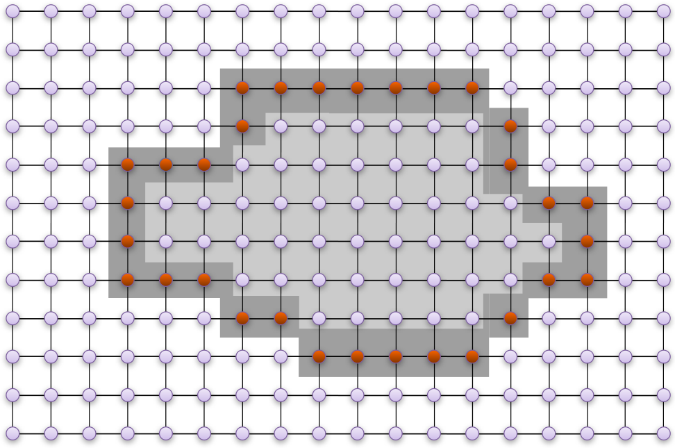
Refer to caption — Figure 3: Schematic representation of a lattice system $L$ , an arbitrary region $R$ (denoted in light grey background), and its boundary $\partial R$ (denoted in dark grey background).

Now, we can add some physics to our lattice by assuming that interactions between the sites of $L$ are governed by some hamiltonian $H$ . We can divide the lattice $L$ into two parts, the region $R$ and its complement $L\setminus R$ . Roughly speaking, we aim to understand how the entropy of the subsystem $R$ scales with its size. In particular, we are interested in the entropy of the state $\varrho_{R}$ reduced from a ground state or a thermal state of the Hamiltonian $H$ . We say that the entropy satisfies an area law if it scales at most as the boundary area¹¹¹¹ 11 Let us shortly recall that the notation $f(x)=O(g(x))$ means that there exist a positive constant $c$ and $x_{0}>0$ such that for any $x\geq x_{0}$ it holds that $f(x)\leq cg(x)$ ., i.e.,

S(\varrho_{R})=O(|\partial R|).

(36)

One-dimensional systems

Let us start with the simplest case of one-dimensional lattices, $L=\{1,\ldots,N\}$ . Let $R$ be a subset of $L$ consisting of $n$ contiguous spins starting from the first site, i.e., $R=\{1,\ldots,n\}$ with $n<N$ . In this case the boundary $\partial R$ of the region $R$ contains one spin for open boundary conditions, and two for periodic ones. Therefore, in this case the area law is extremely simple:

S(\varrho_{R})=O(1).

(37)

The case of $D=1$ seems to be quite well understood. In general, all local gapped systems (away from criticality) satisfy the above law, and there might be a logarithmic divergence of entanglement entropy when the system is critical. To be more precise, let us recall the theorem of Hastings leading to the first of the above statements, followed by examples of critical systems showing a logarithmic divergence of the entropy with the size of $R$ .

Consider the nearest-neighbor interaction Hamiltonian

H=\sum_{i\in L}H_{i,i+1},

(38)

where each $H_{i,i+1}$ has a nontrivial support only on the sites $i$ and $i+1$ . We assume also that the operator norm of all the terms in Eq. (38) are upper bounded by some positive constant $J$ , i.e., $\|H_{i,i+1}\|\leq J$ for all $i$ (i.e., we assume that the interaction strength between $i$ th site and its nearest-neighbor is not greater that some constant). Under these assumptions, Hastings proved the following [78]:

Theorem 3.2

Let $L$ be a one-dimensional lattice with $N$ $d$ -dimensional sites, and let $H$ be a local Hamiltonian as in Eq. (38). Assuming that $H$ has a unique ground state separated from the first excited states by the energy gap $\Delta E>0$ , the entropy of any region $R$ satisfies

S(\varrho_{R})\leq 6c_{0}\xi 2^{6\xi\log d}\log\xi\log d

(39)

with $c_{0}$ denoting some constant of the order of unity and $\xi=\min\{2v/\Delta E,\xi_{C}\}$ . Here, $v$ denotes the sound velocity and is of the order of $J$ , while $\xi_{C}$ is a length scale of order unity.

Let us remark that both constants appearing in the above theorem come from the Lieb-Robinson bound [79] (see also Ref. [80] for a recent simple proof of this bound).

This theorem tells us that when the one-dimensional system with the local interaction defined by Eq. (38) is away from the criticality $(\Delta E>0)$ , the entropy of $R$ is bounded by some constant independent of $|R|$ — even if this bound does not have to be tight. Of course, we can naturally ask if there exist gapped systems with long-range interaction violating (37). This was answered in the affirmative in Ref. [81, 82], which gave examples of one-dimensional models with long–range interactions, nonzero energy gap, and scaling of entropy diverging logaritmically with $n$ .

The second question one could pose is about the behavior of the entropy when the gap $\Delta E$ goes to zero and the system becomes critical. Numerous analytical and numerical results show that usually one observes a logarithmic divergence of $S(\varrho_{R})$ with the size of the region $R$ . Here we recall only the results obtained for the so–called XY model in a transverse magnetic field (for the remaining ones we refer the reader to recent reviews [69, 83], and to the special issue of J. Phys. A devoted to this subject [70]).

The Hamiltonian for the XY model reads

H_{XY}=-\frac{1}{2}\sum_{i\in L}\left(\frac{1+\gamma}{2}\sigma_{i}^{x}\sigma_{i+1}^{x}+\frac{1-\gamma}{2}\sigma_{i}^{y}\sigma_{i+1}^{y}\right)-\frac{h}{2}\sum_{i\in L}\sigma_{i}^{z},

(40)

with $0\leq\gamma\leq 1$ the anisotropy parameter, and $h$ the magnetic field. In the case of vanishing anisotropy ( $\gamma=0$ ), we have the isotropic XY model called shortly XX model, while for $\gamma=1$ one recovers the well–known Ising Hamiltonian in a transverse field. The Hamiltonian $H_{XY}$ is critical when either $\gamma=0$ and $|h|\leq 1$ (the critical XX model) or for $|h|=1$ .

It was shown in a series of papers [84, 85, 86, 87] that for the critical XY model (that is when $\gamma\neq 0$ and $|h|=1$ ) the entropy of the region $R=\{1,\ldots,n\}$ scales as

S(\varrho_{R})=\frac{1}{6}\log_{2}n+O(1),

(41)

while for the critical XX model, the constant multiplying the logarithms becomes one–third. Then, in the case of the critical Ising model ( $\gamma=1$ ), it can be shown that the entropy scales at least logaritmically¹²¹² 12 The notation $f(x)=\Omega(g(x))$ means that there exist $c>0$ and $x_{0}>0$ such that $f(x)\geq cg(x)$ for all $x\geq x_{0}$ ., i.e., $S(\varrho_{R})=\Omega(\log_{2}n)$ [69, 88].

Concluding, let us mention that there is an extensive literature on the logarithmic scaling of the block entropy using conformal field theory methods (see Ref. [89] for a very good overview of these results). Quite generally, the block entropy at criticality scales as

S(\varrho_{R})=\frac{c}{3}\log_{2}\left(\frac{|R|}{a}\right)+O(1),

(42)

or, more in general for the Rényi entropy¹³¹³ 13 Recall that the quantum Rényi entropy is defined as $S_{\alpha}=\frac{1}{1-\alpha}\log_{2}\left[\mathrm{Tr}\left(\varrho^{\alpha}\right)\right]$ (43) where $\alpha\in[0,\infty]$ . For $\alpha=0$ one has $S_{0}(\varrho)=\log_{2}\mathrm{rank}(\varrho)$ and $S_{\infty}=-\log_{2}\lambda_{\mathrm{max}}$ with $\lambda_{\mathrm{max}}$ being the maximal eigenvalue of $\varrho$ .

S_{\alpha}(\varrho_{R})=(c/6)\left(1+1/\alpha\right)\log_{2}(|R|/a)+O(1),

(44)

where $c$ is called the central charge of the underlying conformal field theory, and $a$ is the cutoff parameter (the lattice constant for lattice systems).

Higher–dimensional systems

The situation is much more complex in higher spatial dimensions $(D>1)$ . The boundary $\partial R$ of the general area law, Eq. (36), is no longer a simple one or two–element set and can have a rather complicated structure. Even if there are no general rules discovered so far, it is rather believed that (36) holds for ground states of local gapped Hamiltonians. This intuition is supported by results showing that for quadratic quasifree fermionic and bosonic lattices the area law (36) holds [69]. Furthermore, for critical fermions the entropy of a cubic region $R=\{1,\ldots,n\}^{D}$ is bounded as $\gamma_{1}n^{D-1}\log_{2}n\leq S(\varrho_{R})\leq\gamma_{2}n^{D-1}(\log_{2}n)^{2}$ with $\gamma_{i}$ $(i=1,2)$ denoting some constants [90, 91, 92]. Let us notice that the proof of this relies on the fact that logarithmic negativity (see Eq. (21)) upper bounds the von Neumann entropy, i.e., for any pure bipartite state $|\psi_{AB}\rangle$ , the inequality $S(\varrho_{A(B)})\leq E_{N}(|\psi_{AB}\rangle)$ holds. This in turn is a consequence of monotonicity of the Rényi entropy $S_{\alpha}$ with respect to the order $\alpha$ , i.e., $S_{\alpha}\leq S_{\alpha^{\prime}}$ for $\alpha\geq\alpha^{\prime}$ . This is one of the instances where insights from quantum information help to deal with problems in many–body physics.

Interestingly, very recently Masanes [80] showed that the ground state (and also low–energy eigenstates) entropy of a region $R$ (even a disjoint one) always scales at most as the size of the boundary of $R$ with some correction proportional to $(\log|R|)^{D}$ — as long as the Hamiltonian $H$ is of the local form

H=\sum_{i\in L}H_{i},

(45)

where each $H_{i}$ has nontrivial support only on the nearest-neighbors of the $i$ th site, and satisfies as previously $\|H_{i}\|\leq J$ for some $J>0$ . Thus, the behavior of entropy which is considered to be a violation of the area law (36) can in fact be treated as an area law itself. This is because in this case¹⁴¹⁴ 14 It should be noticed that one can have much stronger condition for such scaling of entropy. To see this explicitly, say that $R$ is a cubic region $R=\{1,\ldots,n\}^{D}$ meaning that $|\partial R|=n^{D-1}$ and $|R|=n^{D}$ . Then since $\lim_{n\to\infty}[(\log n)/n^{\epsilon}]=0$ for any (even arbitrarily small) $\epsilon>0$ , one easily checks that $S(\varrho_{R})/|\partial R|^{1+\epsilon}\to 0$ for $|\partial R|\to\infty$ . $[|\partial R|(\log|R|)^{k}]/|R|\to 0$ for $|R|\to\infty$ with some $k>0$ , meaning that still this behavior of entropy is very different from the typical behavior following from theorem 3.1. That is, putting $m=d^{|R|}$ and $n=d^{|L\setminus R|}$ with $|L|\gg|R|$ one has that $S(\varrho_{R})/|R|$ is arbitrarily close to $\log d$ for large $|R|$ .

Let $R_{1}$ and $R_{2}$ be two disjoint regions of the lattice such that $|R_{1}|\leq|R_{2}|$ , and let $l$ denote the distance between these regions. Let us call $\Gamma$ a function that bounds from above the correlations between two operators $X$ and $Y$ ( $\|X\|,\|Y\|\leq 1$ ) acting respectively on $R_{1}$ and $R_{2}$ , i.e., $C(X,Y)=|\langle XY\rangle-\langle X\rangle\langle Y\rangle|\leq\Gamma(l,|R_{1}|)$ . The first assumption leading to the results of Ref. [80] is that if the mean values in $C$ are taken in the ground state of $H$ , $\Gamma$ is given by

\Gamma(l,|R_{1}|)=c_{1}(l-\xi\log|R_{1}|)^{-\mu}

(46)

with some constants $c_{1}$ , $\xi$ , and $\mu>D$ . Notice that this function decays polynomially in $l$ , meaning that this first assumption is weaker than the property of exponential decay observed in Ref. [93] for gapped Hamiltonians.

Let now $H_{R}$ denote a part of the global Hamiltonian $H$ which acts only on sites in some region $R$ . It has its own eigenvalues and eigenstates, denoted by $e_{n}$ and $|\psi_{n}\rangle$ respectively, with $e_{0}$ denoting the lowest eigenvalue. The second assumption made in Ref. [80] is that there exist constants $c_{2}$ , $\tau$ , $\gamma$ , and $\eta$ such that for any region $R$ and energy $e=2J3^{D}|\partial R|+e_{0}+40v$ (notice that $3^{D}$ is the number of the first neighbours in a cubic lattice), the number of eigenenergies of $H_{R}$ lower than $e$ is upper bounded as

\Omega_{R}(e)\leq c_{2}(\tau|R|)^{\gamma(e-e_{0})+\eta|\partial R|}.

(47)

Now, we are in position to formulate the main result of Ref. [80].

Theorem 3.3

Let $R$ be some arbitrary (even disjoint) region of $L$ . Then, provided the assumptions (46) and (47) hold, the entropy of the reduced density matrix $\varrho_{R}$ of the ground state of $H$ satisfies

S(\varrho_{R})\leq C|\partial R|(10\xi\log|R|)^{D}+O(|\partial R|(\log|R|)^{D-1}),

(48)

where $C$ collects the constants $D,\xi,\gamma,J,\eta$ , and $d$ . If $R$ is a cubic region, the above statement simplifies, giving $S(\varrho_{R})\leq\widetilde{C}|\partial R|\log|R|+O(|\partial R|)$ with $\widetilde{C}$ being some constant.

Leaving out the first assumption, however, at the cost of extending the second assumption to all energies $e$ (not only the ones bounded by $2J3^{D}|\partial R|+e_{0}+40v$ ), leads to the following simple area law:

Theorem 3.4

Let $R$ be an arbitrary region of the lattice $L$ . Assuming that the above number of eigenvalues $\Omega_{R}(e)$ satisfies condition (47) for all $e$ , then

S(\varrho_{R})\leq C|\partial R|\log|R|+O(|\partial R|).

(49)

Proof

Let $|\psi_{i}\rangle$ and $e_{i}$ denote the eigenvectors and ordered eigenvalues $(e_{0}\leq e_{1}\leq\ldots\leq e_{n}\leq\ldots)$ of $H_{R}$ . Then, it is clear that the ground state $|\Psi_{0}\rangle$ of $H$ can be written as $|\Psi_{0}\rangle=\sum_{i,j}\alpha_{ij}|\psi_{i}\rangle|\varphi_{j}\rangle$ , where the vectors $|\varphi_{j}\rangle$ constitute some basis in the Hilbert space corresponding to the region $L\setminus R$ . One may always denote $\sqrt{\mu_{i}}|\widetilde{\varphi}_{i}\rangle=\sum_{j}\alpha_{ij}|\varphi_{j}\rangle$ , and then

|\Psi_{0}\rangle=\sum_{i}\sqrt{\mu_{i}}\,|\psi_{i}\rangle|\widetilde{\varphi}_{i}\rangle,

(50)

where $\mu_{i}=1/\langle\widetilde{\varphi}_{i}|\widetilde{\varphi}_{i}\rangle=1/\sum_{j}|\alpha_{ij}|^{2}\geq 0$ and they add up to unity. The vectors $|\widetilde{\varphi}_{i}\rangle$ in general do not have to be orthogonal, therefore Eq. (50) should not the confused with the Schmidt decomposition of $|\Psi_{0}\rangle$ . Nevertheless, one may show that tracing out the $L\setminus R$ subsystem the entropy of the density matrix acting on $R$ is upper bounded as (see Ref. [52])

S(\varrho_{R})\leq-\sum_{i}\mu_{i}\log\mu_{i}.

(51)

We now aim to maximize the right-hand side of the above equation under the following conditions imposed on $\mu_{i}$ : First, the locality of our Hamiltonian means that $\langle H_{R}\rangle\leq e_{0}+J3^{D}|\partial R|$ , implying that the probabilities $\mu_{i}$ obey

\sum_{i}\mu_{i}\widetilde{e}_{i}\leq J3^{D}|\partial R|,

(52)

with $\widetilde{e}_{i}=e_{i}-e_{0}$ . Second, the modified version of the second assumption allows to infer that for any eigenvalues $e_{i}$ the inequality $i\leq c_{2}(\tau|R|)^{\gamma\widetilde{e}_{i}+\eta|\partial R|}$ holds. Substitution of the above in Eq. (52) gives

\sum_{i}\mu_{i}\log i\leq C|\partial R|\log|R|+O(|\partial R|)

(53)

where $C$ contains the constants $\eta,\gamma,J$ , and $D$ . Eventually, following the standard convex optimization method (see e.g. Ref. [94]) with two constraints (normalization and the inequality (53)) one gets (49). $\blacksquare$

Are laws for mutual information - classical and quantum Gibbs states

So far, we considered area laws only for ground states of local Hamiltonians. In addition, it would be very interesting to ask similar questions for nonzero temperatures. Here, however, one cannot rely on the entropy of a subsystem, as in the case of mixed states it looses its meaning. A very good quantity measuring the total amount of correlation in bipartite quantum systems is the quantum mutual information [95] defined as

I(A:B)=S(\varrho_{A})+S(\varrho_{B})-S(\varrho_{AB}),

(54)

where $\varrho_{AB}$ is some bipartite state with its subsystems $\varrho_{A(B)}$ . It should be noticed that for pure states the mutual information reduces to twice the amount of entanglement of the state.

Recently, it was proven that thermal states $\varrho_{\beta}=e^{-\beta H}/\mathrm{tr}[e^{-\beta H}]$ with local Hamiltonians $H$ obey an area law for mutual information. Interestingly, a similar conclusion was drawn for classical lattices, in which at each site we have a classical spin with the configuration space $\mathbb{Z}_{d}$ , and instead of density matrices one deals with probability distributions. In the following we review these two results, starting from the classical case.

To quantify correlations in classical systems, we use the classical mutual information, defined as in Eq. (54) with the von Neumann entropy substituted by the Shannon entropy $H(X)=-\sum_{x}p(x)\log_{2}p(x)$ , where $p$ stands for a probability distribution characterizing random variable $X$ . More precisely, let $A$ and $B=S\setminus A$ denote two subsystems of some classical physical system $S$ . Then, let $p(x_{A})$ and $p(x_{B})$ be the marginals of the joint probability distribution $p(x_{AB})$ describing $S$ ( $x_{a}$ denotes the possible configurations of subsystems $a=A,B,AB$ ). The correlations between $A$ and $B$ are given by

I(A:B)=H(A)+H(B)-H(AB).

(55)

We are now ready to formulate and prove the following theorem [96].

Theorem 3.5

Let $L$ be a lattice with $d$ –dimensional classical spins at each site. Let $p$ be a Gibbs probability distribution coming from finite–range interactions on $L$ . Then, dividing $L$ into regions $A$ and $B$ , one has

I(A:B)\leq|\partial A|\log d.

(56)

Proof

First, notice that the Gibbs distributions coming from finite–range interactions have the property that if a region $C$ separates $A$ from $B$ in the sense that no interaction is between $A$ and $B$ then $p(x_{A}|x_{C},x_{B})=p(x_{A}|x_{C})$ , which we rewrite as

p(x_{A},x_{B},x_{C})=\frac{p(x_{A},x_{C})p(x_{B},x_{C})}{p(x_{C})}.

(57)

Now, let $A$ and $B$ be two regions of $L$ , and let $\partial A\subset A$ and $\partial B\subset B$ be boundaries of $A$ and $B$ , respectively, collecting all sites interacting with their exteriors. Finally, let $\overline{A}=A\setminus\partial A$ and $\overline{B}=B\setminus\partial B$ . Since $\partial A$ separates $A$ from $\partial B$ (there is no interaction between $A$ and $\partial B$ ), we can use Eq. (57) to obtain

$\displaystyle H(AB)$	$\displaystyle=$	$\displaystyle H(\bar{A}\partial AB)=-\sum_{x_{\bar{A}},x_{\partial A},x_{B}}p(x_{\bar{A}},x_{\partial A},x_{B})\log_{2}p(x_{\bar{A}},x_{\partial A},x_{B})$	(58)
	$\displaystyle=$	$\displaystyle-\sum_{x_{\bar{A}},x_{\partial A}}p(x_{\bar{A}},x_{\partial A})\log_{2}p(x_{\bar{A}},x_{\partial A})$
		$\displaystyle-\sum_{x_{\partial A},x_{B}}p(x_{\partial A},x_{B})\log_{2}p(x_{\partial A},x_{B})$
		$\displaystyle+\sum_{x_{\partial A}}p(x_{\partial A})\log_{2}p(x_{\partial A})$
	$\displaystyle=$	$\displaystyle H(A)+H(\partial AB)-H(\partial A).$

Since $\partial B$ separates $\partial A$ from $B$ , the same reasoning may be applied to the second term of the right-hand side of the above, obtaining $H(\partial AB)=H(\partial A\partial B)+H(B)-H(\partial B)$ . This, together with Eq. (58), gives

H(AB)=H(A)+H(B)+H(\partial A\partial B)-H(\partial A)-H(\partial B),

(59)

which in turn after application to Eq. (55) allows us to write

I(A:B)=I(\partial A:\partial B).

(60)

It means that whenever the probability distribution $p$ has the above Markov property, correlations between $A$ and $B$ are the same as between their boundaries.

Now, we know that the mutual information can be expressed through the conditional Shannon entropy¹⁵¹⁵ 15 The conditional Shannon entropy is defined as $H(A|B)=H(A,B)-H(B)$ . as $I(X:Y)=H(X)-H(X|Y)$ . Since $H(X|Y)$ is always nonnegative, we have the following inequality

I(\partial A:\partial B)\leq H(\partial A)\log d.

(61)

To get Eq. (56) it suffices to notice that $H(A)$ is upper bounded by the Shannon entropy of independently and identically distributed probability $p(x_{A})=1/d^{|A|}$ , which means that $H(A)\leq|A|\log d$ . $\blacksquare$

Let us now show that a similar conclusion can be drawn in the case of quantum thermal states [96], where the Markov property does not hold in general.

Theorem 3.6

Let $L$ be a lattice consisting of $d$ -dimensional quantum systems divided into parts $A$ and $B$ ( $L=A\cup B$ ). Thermal states $(T>0)$ of local Hamiltonians $H$ obey the following area law

I(A:B)\leq\beta\mathrm{tr}[H_{\partial}(\varrho_{A}\otimes\varrho_{B}-\varrho_{AB})].

(62)

Proof

The thermal state $\varrho_{\beta}=e^{-\beta H}/\mathrm{tr}(e^{-\beta H})$ minimizes the free energy $F(\varrho)=\mathrm{tr}(H\varrho)-(1/\beta)S(\varrho)$ , and therefore $F(\varrho_{\beta})\leq F(\varrho^{A}_{\beta}\otimes\varrho^{B}_{\beta})$ with $\varrho^{A}_{\beta}$ and $\varrho^{B}_{\beta}$ subsystems of $\varrho_{\beta}$ . This allows us to estimate the entropy of the thermal state as

$\displaystyle S(\varrho_{\beta})$	$\displaystyle=$	$\displaystyle\beta\left[\mathrm{tr}(H\varrho_{\beta})-F(\varrho_{\beta})\right]$	(63)
	$\displaystyle\geq$	$\displaystyle\beta\left[\mathrm{tr}(H\varrho_{\beta})-F(\varrho^{A}_{\beta}\otimes\varrho^{B}_{\beta})\right]$
	$\displaystyle=$	$\displaystyle\beta\left[\mathrm{tr}(H\varrho_{\beta})-\mathrm{tr}(H\varrho_{\beta}^{A}\otimes\varrho_{\beta}^{B})\right]+S(\varrho_{\beta}^{A}\otimes\varrho_{\beta}^{B})$
	$\displaystyle=$	$\displaystyle\beta\left[\mathrm{tr}(H\varrho_{\beta})-\mathrm{tr}(H\varrho_{\beta}^{A}\otimes\varrho_{\beta}^{B})\right]+S(\varrho_{\beta}^{A})+S(\varrho_{\beta}^{B}),$

where the last equality follows from additivity of the von Neumann entropy $S(\rho\otimes\sigma)=S(\rho)+S(\sigma)$ . Putting Eq. (63) into the formula for mutual information we get

I(A:B)\leq\beta\left[\mathrm{tr}(H\varrho_{\beta}^{A}\otimes\varrho_{\beta}^{B})-\mathrm{tr}(H\varrho_{\beta})\right].

(64)

Let us now write the Hamiltonian as $H=H_{A}+H_{\partial}+H_{B}$ , where $H_{A}$ and $H_{B}$ denote all the interaction terms within the regions $A$ and $B$ , respectively, while $H_{\partial}$ stands for interaction terms connecting these two regions. Then one immediately notices that $\mathrm{tr}[H_{A(B)}(\varrho_{\beta}^{A}\otimes\varrho_{\beta}^{B}-\varrho_{\beta})]=0$ and only the $H_{\partial}$ part of the Hamiltonian $H$ contributes to the right-hand side of Eq. (64). This finishes the proof. $\blacksquare$

Let us notice that the right–hand side of Eq. (62) depends only on the boundary, and therefore it gives a scaling of mutual information similar to the classical case (61). Moreover, for the nearest-neighbor interaction, Eq. (62) simplifies to $I(A:B)\leq 2\beta\|h\|\,|\partial A|$ with $\|h\|$ denoting the largest eigenvalue of all terms of $H$ crossing the boundary.

4 The tensor network product world

Quantum many-body systems are, in general, difficult to describe: specifying an arbitrary state of a system with $N$ -two level subsystems requires $2^{N}$ complex numbers. For a classical computer, this presents not only storage problems, but also computational ones, since simple operations like calculating the expectation value of an observable would require an exponential number of operations. However, we know that completely separable states can be described with about $N$ parameters — indeed, they correspond to classical states. Therefore, what makes a quantum state difficult to describe are quantum correlations, or entanglement. We saw already that even if in general the entropy of a subsystem of an arbitrary state is proportional to the volume, there are some special states which obey an entropic area law. Intuitively, and given the close relation between entropy and information, we could expect that states that follow an area law can be described (at least approximately) with much less information than a general state. We also know that such low entanglement states are few, albeit interesting — we only need an efficient and practical way to describe and parameterize them.

4.1 The tensor network representation of quantum states

Consider a general state of a system with $N$ $d$ -level particles,

|\psi\rangle=\sum_{i_{1},i_{2},\ldots,i_{N}=1}^{d}c_{i_{1}i_{2}\ldots i_{N}}|i_{1},i_{2},\ldots,i_{N}\rangle.

(65)

When the state has no entanglement, then $c_{i_{1}i_{2}\ldots i_{N}}=c^{(1)}_{i_{1}}c^{(2)}_{i_{2}}\ldots c^{(N)}_{i_{N}}$ where all $c$ ’s are scalars. The locality of the information (the set of coefficients $c$ for each site is independent of the others) is key to the efficiency with which separable states can be represented. How can we keep this locality while adding complexity to the state, possibly in the form of correlations but only to nearest-neighbors? As we shall see, we can do this by using a tensor at each site of our lattice, with one index of the tensor for every physical neighbor of the site, and another index for the physical states of the particle. For example, in a one-dimensional chain we would assign a matrix for each state of each particle, and the full quantum state would write as

|\psi\rangle=\sum_{i_{1},i_{2},\ldots,i_{N}=1}^{d}{\rm tr}\left[A^{[1]}_{i_{1}}A^{[2]}_{i_{2}}\ldots A^{[N]}_{i_{N}}\right]|i_{1},i_{2},\ldots i_{N}\rangle,

(66)

where $A^{[k]}_{i_{k}}$ stands for a matrix with dimensions $D_{k}\times D_{k+1}$ . A useful way of understanding the motivations for this representation is to think of a valence bond picture [97]. Imagine that we replace every particle at the lattice by a pair (or more in higher dimensions) of particles of dimensions $D$ that are in a maximally entangled state with their corresponding partners in a neighboring site (see Figure 4). Then, by applying a map from this virtual particles into the real ones,

{\cal A}=\sum_{i=1}^{d}\sum_{\alpha,\beta=1}^{D}A_{\alpha,\beta}^{[i]}|i\rangle\!\langle\alpha,\beta|,

(67)

we obtain a state that is expressed as Eq. (66). One can show that any state $|\psi\rangle\in\mathbb{C}^{dN}$ can be written in this way with $D=\max_{m}D_{m}\leq d^{N/2}$ . Furthermore, a matrix product state can always be found such that [98]

•

$\sum_{i}A^{\dagger[k]}_{i}A^{[k]}_{i}=1_{D_{k}}$ , for $1\leq k\leq N$ ,
•

$\sum_{i}A^{\dagger[k]}_{i}\Lambda^{[k-1]}A^{[k]}_{i}=\Lambda^{[k]}$ , for $1\leq k\leq N$ , and
•

For open boundary conditions $\Lambda^{[0]}=\Lambda^{[N]}=1$ , and $\Lambda^{[k]}$ is a $D_{k+1}\times D_{k+1}$ positive diagonal matrix, full rank, with ${\rm tr}\Lambda^{[k]}=1$ .

In fact, $\Lambda^{[k]}$ is a matrix whose diagonal components $\lambda^{k}_{n}$ , $n=1,\ldots,D_{k}$ , are the non-zero eigenvalues of the reduced density matrix obtained by tracing out the particles from $k+1$ to $N$ , i.e., the Schmidt coefficients of a bipartition of the system at site $k$ . A MPS with these properties is said to be in its canonical form [99].

Figure 4: Schematic representation of tensor networks. In panel

(a)

we show the meaning of the elements in the representation, namely the solid line joining two virtual particles in different sites means the maximally entangled state between them, and the grey circle represents the map from virtual particles in the same site to the physical index. In panel

(b)

we see a one-dimensional tensor network or MPS, while in

(c)

we show how the scheme can be extended intuitively to higher dimensions — in the two-dimensional example shown here, a PEPS that contains four virtual particles per physical site.

Therefore, Eq. (66) is a representation of all possible states — still cumbersome. It becomes an efficient representation when the virtual bond dimension $D$ is small, in which case it is typically said that the state has a matrix product state (MPS) representation. In higher dimensions we talk about projected entangled pair states (PEPS) [100]. When entanglement is small (but finite), most of the Schmidt coefficients are either zero or decay rapidly to zero [84]. Then, if $|\psi\rangle$ contains little entanglement, we can obtain a very good approximation to it by truncating the matrices $A$ to a rank $D$ much smaller than the maximum allowed by the above theorem, $d^{N/2}$ . In fact, we can demonstrate the following

Lemma 1

[99] There exists a MPS $|\psi_{D}\rangle$ with bond dimension $D$ such that $\||\psi\rangle-|\psi_{D}\rangle\|^{2}<2\sum_{\alpha=1}^{N-1}\epsilon_{\alpha}(D)$ , where $\epsilon_{\alpha}(D)=\sum_{i=D+1}^{d^{\min(\alpha,N-\alpha)}}\lambda^{[k]}_{i}$ .

Proof

∎Let us assume that the MPS is in its canonical form with $D=2^{N/2}$ . Defining a projector into the virtual bond dimension $P=\sum_{k=1}^{D}|k\rangle\!\langle k|$ , and a TPCM map $\$_{m}(X)=\sum_{i}A^{[m]\dagger}_{i}XA^{[m]}_{i}$ , we can write the overlap

\langle\psi|\psi_{D}\rangle={\rm Tr}\left[\$_{2}(\ldots\$_{N-2}(\$_{N-1}(\Lambda^{[N-1]}P)P)P)\ldots)P\right].

(68)

By defining $Y^{[k]}=\$_{k}(Y^{[k+1]}P)$ , with $Y^{[N-1]}=\Lambda^{[N-1]}P$ , and using that ${\rm Tr}|\$(X)|\leq{\rm Tr}|X|$ , we can see that

	$\displaystyle\mathrm{tr}\big\|\Lambda^{[k]}-Y^{[k]}\big\|$	$\displaystyle=$	$\displaystyle\mathrm{tr}\big\|\$_{k}(\Lambda^{[k+1]}-Y^{[k+1]}P)\big\|$		(69)
		$\displaystyle\leq$	$\displaystyle\mathrm{tr}\big\|\Lambda^{[k+1]}-Y^{[k+1]}\big\|+\mathrm{tr}\big\|\Lambda^{[k+1]}(1-P)\big\|,$		(69)

where the last term is equal to $\sum_{\alpha=D+1}^{2^{N/2}}\lambda^{[k]}_{\alpha}$ . Finally, applying this last inequality recursively from $N-1$ to $2$ , and using that $\langle\psi_{D}|\psi_{D}\rangle\leq 1$ , we can obtain the desired bound on $\langle\psi|\psi_{D}\rangle$ . ∎

Lemma (1) is most powerful in the context of numerical simulations of quantum states: it gives a controllable handle on the precision of the approximation by MPS. In practical terms, for the representation to be efficient the Schmidt coefficients $\lambda$ need to decay faster than polynomially. However, we can be more precise and give bounds on the error of the approximation in terms of entropies [101]:

Lemma 2

Let $S_{\alpha}(\rho)=\log(\mathrm{tr}\rho^{\alpha})/(1-\alpha)$ be the Rényi entropy of a reduced density matrix $\rho$ , with $0<\alpha<1$ . Denote $\epsilon(D)=\sum_{i=D+1}^{\infty}\lambda_{i}$ , with $\lambda_{i}$ being the eigenvalues of $\rho$ in nonincreasing order. Then,

\log(\epsilon(D))\leq\frac{1-\alpha}{\alpha}\left(S_{\alpha}(\rho)-\log\frac{D}{1-\alpha}\right).

(70)

The question now is when can we find systems with relevant states that can be written efficiently as a MPS; i.e. how broad is the simulability of quantum states by MPS. For example, one case of interest where we could expect the method to fail is near quantum critical points where correlations (and entanglement) are singular and might diverge. However, at least in 1D systems, we can state the following:

Lemma 3

[99] In one dimension there exists a scalable, efficient MPS representation of ground states even at criticality.

Proof

In one dimension, the worst case growth of entropy of a subsystem of size $L$ , exactly at criticality, is given by

S_{\alpha}(\rho_{L})\simeq\frac{c+\tilde{c}}{12}\left(1+\frac{1}{\alpha}\right)\log L.

(71)

Let us take the length $L$ to be half the chain, $N=2L$ . By means of the previous discussion, we can find a MPS $|\psi_{D}\rangle$ such that its distance with the ground state $|\psi_{GS}\rangle$ is bounded as $\||\psi_{GS}\rangle-|\psi_{D}\rangle\|^{2}\leq\epsilon_{0}/L$ , with $\epsilon_{0}$ constant. Now, let $D_{L}$ be the minimal virtual bond dimension needed for this precision, i.e. $\||\psi_{GS}\rangle-|\psi_{D}\rangle\|^{2}\leq 2\times 2L\ \epsilon_{max}(D)$ . We demand that

	$\displaystyle\epsilon_{max}(D)$	$\displaystyle\leq$	$\displaystyle\frac{\epsilon_{0}}{4L^{2}}$		(72)
		$\displaystyle\leq$	$\displaystyle\exp\left[\frac{1-\alpha}{\alpha}\left(\frac{c+\tilde{c}}{12}\frac{1+\alpha}{\alpha}\log L-\log\frac{D_{L}}{1-\alpha}\right)\right],$		(72)

from which we can extract

D_{L}\leq\mathrm{const}\ \left(\frac{L^{2}}{\epsilon_{0}}\right)^{\frac{\alpha}{1-\alpha}}L^{\frac{c+\tilde{c}}{12}\frac{1+\alpha}{\alpha}}\propto{\rm poly}(L).

(73)

$\blacksquare$

Establishing that there exists an efficient representation of the ground state is not enough: we must also know if it is possible to find it efficiently too. In one dimensional gapped systems, the gap $\Delta$ typically scales polynomially, which means that DMRG and MPS methods should converge reasonably fast. One can, however, formalize the regime of efficiency of MPS as a function of how the different Rényi entropies scale with subsystem size [101]. In table (1) we summarize the currently known regimes where the MPS approach is an appropriate one or not.

$S_{\alpha}\sim$	const	$\log L$	$L^{\kappa}(\kappa<1)$	$L$
$S_{\alpha}<1$	OK	OK	?	?
$S\equiv S_{1}$	?	?	?	NO
$S_{\alpha}>1$	?	?	NO	NO

Table 1: Relation between scaling of block Rényi entropies and approximability by MPS [101]). In the “undetermined” region denoted with question marks, nothing can be said about approximability just from looking at the scaling.

4.2 Examples

Here we present a few models and states that are fine examples of the power of MPS representations[99].

Example 6

A well known model with a finite excitation gap and exponentially decaying spin correlation functions was introduced by Affleck, Kennedy, Lieb, and Tasaki [102, 103]—the so called AKLT model. The model Hamiltonian is

H=\sum_{i}\vec{S}_{i}\cdot\vec{S}_{i+1}+\frac{1}{3}\left(\vec{S}_{i}\cdot\vec{S}_{i+1}\right)^{2}.

(74)

For $S=1$ , the local Hilbert space of each spin has three states, thus $d=3$ . The ground state of this Hamiltonian can be written compactly using a translationally invariant MPS with bond dimension $D=2$ , specifically

A_{-1}=\sigma_{x},\ A_{0}=\sqrt{2}\sigma^{+},\ A_{1}=-\sqrt{2}\sigma^{-}.

(75)

Example 7

A paradigmatic example of a frustrated one dimensional spin chain is the Majumdar-Ghosh [104] model with nearest and next nearest-neighbor interactions:

H=\sum_{i}2\vec{\sigma}_{i}\cdot\vec{\sigma}_{i+1}+\vec{\sigma}_{i}\cdot\vec{\sigma}_{i+2},

(76)

The model is equivalent to the or $J_{1}-J_{2}$ Heisenberg model with $J_{1}/J_{2}=2$ . The ground state of this model is composed of singlets between nearest-neighbor spins. However, since the state must be translationally invariant, we must include a superposition of singlets between even-odd spins, and “shifted” singlets between odd-even spins. The state can be written compactly in MPS form using $D=3$ ,

A_{0}=\left(\begin{array}[]{ccc}0&1&0\\ 0&0&-1\\ 0&0&0\end{array}\right),\ \ A_{1}=\left(\begin{array}[]{ccc}0&0&0\\ 1&0&0\\ 0&1&0\end{array}\right)

(77)

Example 8

A relevant state for quantum information theory is the Greenberger–Horne–Zeilinger (GHZ) state, which for $N$ spin $1/2$ particles can be written as

|GHZ\rangle=\frac{|0\rangle^{\otimes N}+|1\rangle^{\otimes N}}{\sqrt{2}}.

(78)

GHZ states are considered important because for many entanglement measures they are maximally entangled, however by measuring or tracing out any qubit a classical state is obtained (although with correlations). GHZ states can be written using $D=2$ MPS, specifically $A_{0,1}=1\pm\sigma_{z}$ . Also the “antiferromagnetic” GHZ state is simple, $A_{0,1}=\sigma^{\pm}$ .

Example 9

Cluster states are relevant for one-way quantum computing. They are the ground state of

H=\sum\sigma^{z}_{i-1}\sigma^{x}_{i}\sigma^{z}_{i+1},

(79)

and can be represented using a $D=2$ MPS,

A_{0}=\left(\begin{array}[]{cc}0&0\\ 1&1\end{array}\right),\ \ A_{1}=\left(\begin{array}[]{cc}1&-1\\ 0&0\end{array}\right)

(80)

Example 10

(Classical superposition MPS) Imagine we have a classical Hamiltonian

H=\sum_{(i,j)}h(\sigma_{i},\sigma_{j}),

(81)

where $\sigma_{i}=1,\ldots,d$ , and $h(\sigma_{i},\sigma_{j})$ are local interactions. The partition function of such a model at a given inverse temperature $\beta$ is

Z=\sum_{\{\sigma\}}\exp\left[-\beta H(\sigma)\right],

(82)

where the sum is over all possible configurations of the vector $\sigma$ . Let us now define a quantum state $|\psi_{\beta}\rangle$ whose amplitude for a given state of the computational basis corresponds to the term in the partition function for that state, i.e.

	$\displaystyle\|\psi_{\beta}\rangle$	$\displaystyle=$	$\displaystyle\frac{1}{\sqrt{Z}}\sum_{\{\sigma\}}\exp\left[-\frac{\beta}{2}H(\sigma)\right]\|\sigma_{1}\ldots\sigma_{N}\rangle$		(83)
		$\displaystyle=$	$\displaystyle\frac{1}{\sqrt{Z}}\sum_{\{\sigma\}}\prod_{(i,j)}\exp\left[-\frac{\beta}{2}h(\sigma_{i},\sigma_{j})\right]\|\sigma_{1}\ldots\sigma_{N}\rangle.$		(83)

We shall now define a map $P$ —in the same manner as in valence bond states— that goes from $\mathbb{C}^{d^{2}}$ to $\mathbb{C}^{2}$ such that

P|s,k\rangle=|s\rangle\langle\varphi_{s}|k\rangle,

(84)

where we have defined

\sum_{\alpha=1}^{d}\langle\varphi_{s}|\alpha\rangle\langle\varphi_{\tilde{s}}|\alpha\rangle=\exp\left[-\frac{\beta}{2}h(s,{\tilde{s}})\right].

(85)

To visualize what happens when we insert these back into the classical superposition state $|\psi_{\beta}\rangle$ , let us concentrate for a moment on a one-dimensional system:

$\displaystyle\|\psi_{\beta}\rangle$	$\displaystyle=$	$\displaystyle\frac{1}{\sqrt{Z}}\sum_{\sigma_{1},\ldots,\sigma_{N}}\exp\left[-\frac{\beta}{2}h(\sigma_{1},\sigma_{2})\right]\ldots\exp\left[-\frac{\beta}{2}h(\sigma_{N-1},\sigma_{N})\right]\|\sigma_{1}\ldots\sigma_{N}\rangle,$
$\displaystyle\|\psi_{\beta}\rangle$	$\displaystyle=$	$\displaystyle\frac{1}{\sqrt{Z}}\sum_{\sigma_{1},\ldots,\sigma_{N}}\left(\sum_{\alpha_{1}=1}^{d}\langle\varphi_{\sigma_{1}}\|\alpha_{1}\rangle\langle\varphi_{\sigma_{2}}\|\alpha_{1}\rangle\sum_{\alpha_{2}=1}^{d}\langle\varphi_{\sigma_{2}}\|\alpha_{2}\rangle\langle\varphi_{\sigma_{3}}\|\alpha_{2}\rangle\right.$	(86)
		$\displaystyle\hskip 65.44142pt\left.\times\ldots\times\sum_{\alpha_{N}=1}^{d}\langle\varphi_{\sigma_{N}}\|\alpha_{N}\rangle\langle\varphi_{\sigma_{1}}\|\alpha_{N}\rangle\right)\|\sigma_{1}\ldots\sigma_{N}\rangle,$	(86)
$\displaystyle\|\psi_{\beta}\rangle$	$\displaystyle=$	$\displaystyle\frac{1}{\sqrt{Z}}\sum_{\sigma_{1},\ldots,\sigma_{N}}\sum_{\alpha_{1},\ldots,\alpha_{N}=1}^{d}\left[\langle\varphi_{\sigma_{1}}\|\alpha_{N}\rangle\langle\varphi_{\sigma_{1}}\|\alpha_{1}\rangle\right]\left[\langle\varphi_{\sigma_{2}}\|\alpha_{1}\rangle\langle\varphi_{\sigma_{2}}\|\alpha_{2}\rangle\right]$	(87)
		$\displaystyle\hskip 98.16191pt\times\ldots\times\left[\langle\varphi_{\sigma_{N}}\|\alpha_{N-1}\rangle\langle\varphi_{\sigma_{N}}\|\alpha_{N}\rangle\right]\|\sigma_{1}\ldots\sigma_{N}\rangle,$	(87)

and we can replace $A^{(i)}_{s_{i},\alpha,\beta}=\langle\varphi_{s_{i}}|\alpha\rangle\langle\varphi_{s_{i}}|\beta\rangle$ , thus expressing the classical thermal superposition state as a MPS.

These states have some important properties:

(i)

They obey strict area laws,
(ii)

They allow to calculate classical and quantum correlations, and
(iii)

They are ground states of local Hamiltonians.

Property (i) should be obvious by now, since we have explicitly shown the MPS form of the state. We can show easily property (ii) for Ising models. A classical correlation function $f$ must be evaluated with the partition function, $\langle f(\sigma)\rangle=\sum_{\sigma}f(\sigma)e^{-\beta H(\sigma)}/Z$ , but this is just the expectation value of an operator made of changing the argument of $f$ into $\sigma_{z}$ operators, and evaluated with $|\psi_{\beta}\rangle$ . Since it is the expectation value of a MPS, it is efficient to compute. Finally, we will demonstrate property (iii) at length in the next section, because it will lead us into the final topic of this lectures: Quantum kinetic models.

4.3 Classical kinetic models

Our goal in this section is to show the local Hamiltonians whose ground state is the classical superposition state defined in the previous section. As we shall see, these Hamiltonians will arise from the master equation of a classical system that is interesting in its own right, so we will first spend some time on it.

Let us consider a system made out of $N$ classical spins interacting through a Hamiltonian $H$ . If $\sigma_{i}$ denotes the state of $i$ th spin, we will label the configurations of the system by $\sigma=(\sigma_{1},\ldots,\sigma_{N})$ , and the probability of finding at time $t$ the system in state $\sigma$ (given that it was in state $\sigma_{0}$ at time $t_{0}$ ) by $P(\sigma,t)=P(\sigma,t|\sigma_{0},t_{0})$ . In what follows we focus on this probability distribution, whose dynamics is described by a master equation:

{\dot{P}}(\sigma,t)=\sum_{\sigma^{\prime}}W(\sigma,\sigma^{\prime})P(\sigma^{\prime},t)-\sum_{\sigma^{\prime}}W(\sigma^{\prime},\sigma)P(\sigma,t),

(88)

where $W(\sigma,\sigma^{\prime})$ is the transition probability from state $\sigma^{\prime}$ to state $\sigma$ . This equation defines the class of kinetic models, and it clearly describes a Markov process — the instantaneous change of $P(\sigma,t)$ does not depend on its history.

We will only consider systems that obey a detailed balance condition, i.e.

W(\sigma,\sigma^{\prime})e^{-\beta H(\sigma^{\prime})}=W(\sigma^{\prime},\sigma)e^{-\beta H(\sigma)}.

(89)

With this condition, the stationary state of the master equation (the one that fulfills ${\dot{P}}_{\mathrm{st}}(\sigma,t)=0$ ) is simply $P_{\mathrm{st}}(\sigma)=e^{-\beta H(\sigma)}/Z$ , with $Z$ being the partition function. This state in particular will map into the classical superposition state defined above, but we still have not found its parent Hamiltonian. For this, we will rewrite Eq. (88) in the form of a matrix Schrödinger equation (albeit with imaginary time) from which we can identify a Hamiltonian.

Let us apply the transformation $\psi(\sigma,t)=e^{\beta H(\sigma)/2}P(\sigma,t)$ , which leads to

	$\displaystyle{\dot{\psi}}(\sigma,t)$	$\displaystyle=$	$\displaystyle\sum_{\sigma^{\prime}}e^{\beta H(\sigma)/2}W(\sigma,\sigma^{\prime})e^{-\beta H(\sigma^{\prime})/2}\psi(\sigma^{\prime},t)-W(\sigma^{\prime},\sigma)\psi(\sigma,t)$		(90)
		$\displaystyle=$	$\displaystyle-\sum_{\sigma^{\prime}}H_{\beta}(\sigma,\sigma^{\prime})\psi(\sigma^{\prime},t)$		(90)

with

H_{\beta}(\sigma,\sigma^{\prime})=\sum_{\sigma^{\prime\prime}}W(\sigma^{\prime\prime},\sigma^{\prime})\delta_{\sigma\sigma^{\prime}}-e^{\beta H(\sigma)/2}W(\sigma,\sigma^{\prime})e^{-\beta H(\sigma^{\prime})/2}.

(91)

Notice that the detailed balance condition guarantees that the matrix $H_{\beta}$ is Hermitian, so we can interpret it as a Hamiltonian. Furthermore, because of the conservation of probability, $H_{\beta}$ can only have non-negative eigenvalues, which means that the state $\psi_{\mathrm{st}}$ associated to the stationary state $P_{\mathrm{st}}$ with eigenvalue zero must be a ground state: the classical superposition MPS that we were looking for.

Remarkably, we have not said anything yet about $H$ . A famous example of such kinetic model is a single spin-flip model considered by Glauber [105], for which $H$ is the Ising Hamiltonian¹⁶¹⁶ 16 This is the reason why the Glauber model is also known as the kinetic Ising model (KIM).

H(\sigma)\equiv H_{\mathrm{Ising}}(\sigma)=-J\sum_{\langle i,j\rangle}\sigma_{i}^{z}\sigma_{j}^{z}\qquad(J>0).

(92)

Denoting by $P_{i}$ the flip operator of the $i$ -th spin, i.e., $P_{i}\sigma_{i}=-\sigma_{i}$ , the general master equation (88) reduces in this case to

\dot{P}(\sigma,t)=\sum_{i}\left[W(\sigma,P_{i}\sigma)P(P_{i}\sigma,t)-W(P_{i}\sigma,\sigma)P(\sigma,t)\right]

(93)

with $W(\sigma,P_{i}\sigma)$ now called spin rates. It was shown in [105] that the most general form of spin rates with symmetric interaction with both nearest-neighbors, and satisfying the detailed balance condition (89), is given by

w(P_{i}\sigma,\sigma)=\Gamma(1+\delta\sigma_{i-1}\sigma_{i+1})[1-(1/2)\gamma\sigma_{i}(\sigma_{i-1}+\sigma_{i+1})]

(94)

with $\Gamma>0$ , $-1\leq\delta\leq 1$ , and $0\leq\gamma\leq 1$ . The $\delta=0$ case was thoroughly investigated by Glauber [105], who showed that all the relevant quantities can be derived analytically — including the dynamical exponent that turned out to be $z=2$ . The more general case of nonzero $\delta$ was treated in a series of papers [106, 107, 108], that showed for instance that the choice $\delta=\gamma/(2-\gamma)$ leads to an interesting dynamical exponent $z\neq 2$ .

If we rewrite the single spin-flip master equation in the form of the Schrödinger equation, we obtain an associated quantum Hamiltonian

	$\displaystyle H_{\beta}(\delta,\gamma)$	$\displaystyle=$	$\displaystyle-\Gamma\sum_{i}\left[\left(A(\delta,\gamma)-B(\delta,\gamma)\sigma_{i-1}^{z}\sigma_{i+1}^{z}\right)\sigma_{i}^{x}\right.$
			$\displaystyle\left.\hskip 39.83368pt-(1+\delta\sigma_{i-1}^{z}\sigma_{i+1}^{z})\left(1-(1/2)\gamma\sigma_{i}^{z}\left(\sigma_{i-1}^{z}+\sigma_{i+1}^{z}\right)\right)\right],$

where

A(\delta,\gamma)=\frac{(1+\delta)\gamma^{2}}{2(1-\sqrt{1-\gamma^{2}})}-\delta,\qquad B(\delta,\gamma)=1-A(\delta,\gamma)

(96)

and $\sigma^{z}$ and $\sigma^{x}$ are the standard Pauli matrices. For $\delta=0$ this Hamiltonian was diagonalized in Ref. [109], and independently in Ref. [110].

The Hamiltonian $H_{\beta}(\delta,\gamma)$ , and also the other ones that can be derived in this way, are typically gapped except at a critical temperature $\beta_{c}$ where the gap vanishes with the critical exponent $z$ that characterizes the model. In one dimension $\beta_{c}=\infty$ , but for larger dimensions this model has a finite critical temperature.

We have seen thus far how the the master equation of a classical spin model (that obeys the detailed balance condition) can be associated to a quantum Hamiltonian with some interesting critical properties — for example, its ground state obeys a strict area law and can be written efficiently as a MPS. Nevertheless, the underlying model is still classical. In the next section, we will see one way in which we can generalize the initial model to be quantum, while retaining the same structure that leads to associated Hamiltonians that obey area laws.

5 Quantum kinetic Ising models

Here we discuss ways to generalize the kinetic equation (88) to a quantum master equation, but in such a way that its diagonal part reproduces the corresponding kinetic model. A similar approach was taken in Ref. [111], where a quantum master equation that reproduced a kinetic Ising model was proposed (see also Ref. [112]). However, no attempts aiming at fully solving such QMEs are known so far. Our purpose is to give quantum generalizations of the classical kinetic models that can be solved analytically.

Recently, we presented such a generalization [113] for the single spin-flip model, Eq. (93), with the spin rates of Eq. (94). In Ref. [113] we were able to decouple the master equation for the density matrix of a quantum system into $2^{N}$ master equations with the same structure as the ones studied above. Here, we will only show the associated Hamiltonians (and their spectra) obtained in these models. However, we will demonstrate how to approach the problem but in a different model that allows transitions that flip two consecutive spins.

5.1 A two spin flip model

First, let us particularize the classical kinetic equation (88) to the case where the flip operator acts on pairs of consecutive spins of the chain, i.e.

\frac{\partial P(\sigma,t)}{\partial t}=\sum_{i}\left[w_{i}(F_{i,i+1}\sigma\rightarrow\sigma)P(F_{i,i+1}\sigma,t)-w_{i}(\sigma\rightarrow F_{i,i+1}\sigma)P(\sigma,t)\right],

(97)

where $F_{i,i+1}$ denote spin flips at positions $i$ and $i+1$ , while the spin rates are given by $w_{i}(F_{i,i+1}\sigma,\sigma)=\Gamma[1-(1/2)\gamma(\sigma_{i-1}\sigma_{i}+\sigma_{i+1}\sigma_{i+2})]$ with $0<\Gamma<\infty$ and $\gamma=\tanh 2\beta J$ . This model was investigated in Ref. [114], where the associated Hamiltonian was found and diagonalized using the Jordan-Wigner transformation [115] followed by Fourier and Bogoliubov-Valatin [116, 117] transformations. In particular, Hilhorst et al. were able to show that, despite the complexity of the transformations, one can easily compute expectation values such as magnetization, energy density, or correlations, and that they have a relatively simple exponential behavior [114].

Here we will define through a master equation a quantum model that resembles the kinetic model above. For this, we will replace classical probabilities with the quantum density matrices, and classical operators with quantum ones (e.g. $\sigma^{x}$ is the qubit flip operator). Consider the following master equation

\partial_{t}\varrho(t)=\sum_{i}\left[\sigma_{i}^{x}\sigma_{i+1}^{x}\sqrt{w_{i}(\sigma^{z})}\varrho(t)\sqrt{w_{i}(\sigma^{z})}\,\sigma_{i}^{x}\sigma_{i+1}^{x}-\frac{1}{2}\{w_{i}(\sigma^{z}),\varrho(t)\}\right],

(98)

where $\{\cdot,\cdot\}$ denotes the anticommutator and $w_{i}(\sigma^{z})$ are quantum mechanical generalizations of the spin rates (94), now written in terms of the $\sigma^{z}$ operators,

w_{i}(\sigma^{z})=\Gamma\left[1-\textstyle\frac{1}{2}\gamma(\sigma_{i-1}^{z}\sigma_{i}^{z}+\sigma_{i+1}^{z}\sigma_{i+2}^{z})\right].

(99)

Although it looks complicated, the quantum kinetic model above can still be solved with techniques similar to the classical case [113]: the key ingredient is to find a large number of constants of motion that allow to split the master equation into a set of ordinary Schrödinger equations. To see this, we must represent the density matrix $\varrho(t)$ as a vector in an expanded Hilbert space. This follows from a simple isomorphism between linear operators from $M_{d}(\mathbb{C})$ and vectors from $\mathbb{C}^{d^{2}}$ . In other words, writing our density matrix in the computational basis in $(\mathbb{C}^{2})^{\otimes N}$ as $\varrho(t)=\sum_{\sigma,\widetilde{\sigma}}[\varrho(t)]_{\sigma,\widetilde{\sigma}}|\sigma\rangle\!\langle\widetilde{\sigma}|$ , we can treat it as a vector $|\varrho(t)\rangle=\sum_{\sigma,\widetilde{\sigma}}[\varrho(t)]_{\sigma,\widetilde{\sigma}}|\sigma\rangle|\widetilde{\sigma}\rangle$ from $(\mathbb{C}^{2})^{\otimes N}\otimes(\mathbb{C}^{2})^{\otimes N}$ . Even if formally we are enlarging the number of spins from $N$ to $2N$ , the advantage is that now we deal with “pure states” instead of density matrices which allows us to find many conserved quantities. This, in turn, shows that the effective Hilbert space used is much smaller than the initial one. To be consistent, operators that appear to the right of $\varrho(t)$ must be replaced with “tilded” operators that act on the right subsystem of the expanded space, while operators on the left of the density matrix (“untilded”) act on the left subsystem (for instance $\sigma_{i}^{x}\widetilde{\sigma}_{i}^{x}|s\rangle|\widetilde{s}\rangle=\sigma_{i}|s\rangle\widetilde{\sigma}_{i}^{x}|\widetilde{s}\rangle$ ). This notation allows us to rewrite the master equation (98) as the following matrix equation

|\dot{\varrho}(t)\rangle=\sum_{i}\left[\sigma_{i}^{x}\sigma_{i+1}^{x}\widetilde{\sigma}_{i}^{x}\widetilde{\sigma}_{i+1}^{x}\sqrt{w_{i}(\sigma^{z})w_{i}(\widetilde{\sigma}^{z})}-\frac{1}{2}[w_{i}(\sigma^{z})+w_{i}(\widetilde{\sigma}^{z})]\right]|\varrho(t)\rangle.

(100)

As was the case for the initial classical master equation, the matrix appearing on the right-hand side of Eq. (100) is not Hermitian. In order to bring it to Hermitian form we can use the detailed balance condition, which suggests the transformation

|\varrho(t)\rangle=\exp\left[-(\beta/4)[\mathcal{H}(\sigma)+\mathcal{H}(\widetilde{\sigma})]\right]|\psi(t)\rangle,

(101)

with $\mathcal{H}$ denoting the quantum generalization of the Ising Hamiltonian $\mathcal{H}=-J\sum_{i}\sigma_{i}^{z}\sigma_{i+1}^{z}$ . With this transformation, and denoting

v_{i}(\sigma^{z})=w_{i}(\sigma^{z})\exp[(\beta J)\sigma_{i}^{z}(\sigma_{i-1}^{z}+\sigma_{i+1}^{z})],

(102)

Eq. (100) can be written as

|\dot{\psi}(t)\rangle=\sum_{i}\left[\sigma_{i}^{x}\sigma_{i+1}^{x}\widetilde{\sigma}_{i}^{x}\widetilde{\sigma}_{i+1}^{x}\sqrt{v_{i}(\sigma^{z})v_{i}(\widetilde{\sigma}^{z})}-\frac{1}{2}[v_{i}(\sigma^{z})+v_{i}(\widetilde{\sigma}^{z})]\right]|\psi(t)\rangle

(103)

which we can see as a Schrödinger equation $|\dot{\psi}(t)\rangle=-H|\psi(t)\rangle$ with Hermitian $H$ .

We have reached the point where all these changes of notation payoff: indeed, the form of $H$ makes it clear that it commutes with $\sigma_{i}^{z}\sigma_{i+1}^{z}\widetilde{\sigma}_{i}^{z}\widetilde{\sigma}_{i+1}^{z}$ $(i=1,\ldots,N)$ . Therefore, we can introduce new variables $\tau_{i}=\sigma_{i}^{z}\sigma_{i+1}^{z}\widetilde{\sigma}_{i}^{z}\widetilde{\sigma}_{i+1}^{z}$ $(i=1,\ldots,N)$ which are constants of motion and reduce the number of degrees of freedom. In particular, tilded variables can be expressed by $\sigma$ and the new variables $\tau$ as $\widetilde{\sigma}_{i}^{z}\widetilde{\sigma}_{i+1}^{z}=\tau_{i}\sigma_{i}^{z}\sigma_{i+1}^{z}$ for any $i$ . In other words, we have replaced $\sigma$ and $\widetilde{\sigma}$ by $\tau$ and $\sigma$ , of which $\tau$ is conserved. To each configuration of $\tau$ ’s we associate a natural number from 0 to $2^{N}-1$ , which corresponds to a particular correlation between the $\sigma$ and $\widetilde{\sigma}$ variables. For example, $\tau=0$ corresponds to all $\tau$ -spins up ( $\tau_{i}=1$ for $i=1,\ldots,N$ ), while $\tau=2^{N}-1$ means that $\tau_{i}=-1$ for $i=1,\ldots,N$ . With this notation, each value of $\tau$ is associated to a Hamiltonian $H_{\tau}$ that acts only in the space of $N$ spins and is of the form

\displaystyle H_{\tau}

\displaystyle=

\displaystyle-\sum_{i}\left[\sigma_{i}^{x}[v_{i}(\sigma^{z})]^{\frac{1}{2}}[v_{i}(\tau\sigma^{z})]^{\frac{1}{2}}-\frac{1}{2}[w_{i}(\sigma^{z})+w_{i}(\tau\sigma^{z})]\right],

(104)

where $\tau\sigma^{z}$ denotes $\tau_{i}\sigma_{i}^{z}$ $(i=1,\ldots,N)$ . Because these Hamiltonians are independent from each other, we have converted the problem of solving the general master equation (98) to the problem of diagonalizing $2^{N}$ Hamiltonians, each of dimension $2^{N}\times 2^{N}$ . Now, we have that

|\psi(t)\rangle=\bigotimes_{\tau=0}^{2^{N}-1}|\psi_{\tau}(t)\rangle,\qquad H=\bigotimes_{\tau=0}^{2^{N}-1}H_{\tau}.

(105)

After simple algebra one sees that the explicit form of $H_{\tau}$ is

	$\displaystyle H_{\tau}$	$\displaystyle=$	$\displaystyle-\sum_{i}\Big[\left(A_{i}(\varphi)-B_{i}(\varphi)\sigma_{i-1}^{z}\sigma_{i}^{z}\sigma_{i+1}^{z}\sigma_{i+2}^{z}\right)\sigma_{i}^{x}\sigma_{i+1}^{x}$		(106)
			$\displaystyle\hskip 28.45274pt\left.-\left[1-\frac{1}{2}\gamma\left(f(\tau_{i-1})\sigma_{i-1}^{z}\sigma_{i}^{z}+f(\tau_{i+1})\sigma_{i+1}^{z}\sigma_{i+2}^{z}\right)\right]\right],$		(106)

where

A_{i}(\varphi)=\left\{\begin{array}[]{ll}\cos^{2}\!\varphi,&\;\;\tau_{i-1}\tau_{i+1}=1\\[4.30554pt] \sqrt{\cos 2\varphi},&\;\;\tau_{i-1}\tau_{i+1}=-1\end{array}\right.,\qquad B_{i}(\varphi)=\left\{\begin{array}[]{ll}\sin^{2}\!\varphi,&\;\;\tau_{i-1}\tau_{i+1}=1\\[4.30554pt] 0,&\;\;\tau_{i-1}\tau_{i+1}=-1,\end{array}\right.

(107)

with

\cos\varphi=\frac{\cosh\!\beta J}{(\cosh^{2}\!\beta J+\sinh^{2}\!\beta J)^{1/2}},\qquad\sin\varphi=\frac{\sinh\!\beta J}{(\cosh^{2}\!\beta J+\sinh^{2}\!\beta J)^{1/2}},

(108)

and $f(x)=(1/2)(1+x)$ . Here the angle ranges from zero (which corresponds to infinite temperature) to $\pi/4$ (which corresponds to $T=0$ ) and in this notation $\gamma=\sin 2\varphi$ . Let us notice that for $\tau=0$ Eqs. (106) and (107), as it should be, reproduce the Hamiltonian derived in [114]. This, however, contrary to the single spin-flip case, is not the case for $\tau=2^{N}-1$ , where one of the terms in the square brackets vanishes and the Hamiltonian reduces to

H_{2^{N}-1}=-\sum_{i}\left[\left(A_{i}(\varphi)-B_{i}(\varphi)\sigma_{i-1}^{z}\sigma_{i}^{z}\sigma_{i+1}^{z}\sigma_{i+2}^{z}\right)\sigma_{i}^{x}\sigma_{i+1}^{x}-1\right]

(109)

Let us discuss now some of the properties of $H_{\tau}$ . Below we show that for all $\tau$ they are always positive operators. We also find all the cases with respect to $\varphi$ and $\tau$ for which the Hamiltonians can have zero-energy ground states.

Lemma 4

The Hamiltonians $H_{\tau}$ are positive for any $\tau=0,\ldots,2^{N}-1$ .

Proof

Let us denote by $H_{\tau}^{(i)}$ the $i$ th term appearing in the sum in Eq. (106). The idea is to show that all $H_{\tau}^{(i)}$ are positive, and the positivity of $H_{\tau}$ follows immediately. Of course, the form of $H_{\tau}^{(i)}$ changes depending on $\tau$ -spins at positions $i-1$ and $i+1$ . Therefore, we distinguish several cases with respect to different possible configurations of these spins.

For $\tau_{i-1}=\tau_{i+1}$ , one easily infers from Eqs. (106) and (107) that

	$\displaystyle H_{\tau}^{(i)}$	$\displaystyle=$	$\displaystyle 1-\frac{1}{2}\gamma\left[f(\tau_{i-1})\sigma_{i-1}^{z}\sigma_{i}^{z}+f(\tau_{i+1})\sigma_{i+1}^{z}\sigma_{i+2}^{z}\right]$		(110)
			$\displaystyle-\left(\cos^{2}\!\varphi-\sin^{2}\!\varphi\,\sigma_{i-1}^{z}\sigma_{i}^{z}\sigma_{i+1}^{z}\sigma_{i+2}^{z}\right)\sigma_{i}^{x}\sigma_{i+1}^{x}.$		(110)

In the case when both spins $\tau_{i-1}$ and $\tau_{i+1}$ are down, the function $f$ is zero and both terms in square brackets vanish and the above operator becomes $1-(\cos^{2}\varphi-\sin^{2}\sigma_{i-1}^{z}\sigma_{i}^{z}\sigma_{i+1}^{z}\sigma_{i+2}^{z})\sigma_{i}^{x}\sigma_{i+1}^{x}$ . It is clear then that its minimal eigenvalue is zero. In the case when $\tau_{i-1}=\tau_{i+1}=1$ these terms do not vanish, however, still this is effectively a $16\times 16$ matrix which can be shown to be positive computationally: using the software Mathematica we can easily see that the minimal eigenvalue is zero.

For $\tau_{i-1}=-\tau_{i+1}$ , one of the values $f(\tau_{i-1})$ or $f(\tau_{i+1})$ is zero. Assuming that $f(\tau_{i-1})=0$ (the case of $f(\tau_{i+1})=0$ leads to the same eigenvalues), one has

H_{\tau}^{(i)}=1-\frac{1}{2}\sin 2\varphi\,\sigma_{i+1}^{z}\sigma_{i+2}^{z}-\sqrt{\cos 2\varphi}\,\sigma_{i}^{x}\sigma_{i+1}^{x}.

(111)

When constrained to three consecutive spins ( $i-1$ , $i$ , and $i+1$ ) this $H_{\tau}^{(i)}$ is just a $8$ by $8$ matrix (on the remaining spins it acts as the identity matrix) and its eigenvalues can be obtained using Mathematica. One then checks that its minimal eigenvalue is $1-(1/2)\sqrt{4\cos 2\varphi+(\sin 2\varphi)^{2}}$ with $\varphi\in[0,\pi/4]$ . Simple analysis shows that this is a nonnegative function of $\varphi$ and gives zero only when $\varphi=0$ .

In conclusion, $H_{\tau}^{(i)}\geq 0$ for all $\tau$ s and $\varphi\in[0,\pi/4]$ and therefore our Hamiltonians $H_{\tau}$ are positive. $\blacksquare$

Figure 5: Low energy states of the Hamiltonians (106) associated to the two flip quantum master equation for a system with

N=16

spins as a function of

\varphi

. The panels are (a)

\tau=2^{8}-1

(half

\tau

-spins up and half down), (b)

\tau=2^{8}

(only one

\tau

-spin up, the others down), and (c)

\tau=2^{9}+2^{8}

(two neighboring

\tau

-spins up, the others down). Only in case (c) the ground state is fully degenerate for all values of

\varphi

, in the other two the first excited state energy is very close but not equal to the ground state. In case (b) the ground state is not degenerate at

\varphi=\pi/4

, while in the other two cases it is.

Based on the above analysis, let us now distinguish all the cases with respect to $\tau$ and $\varphi$ when $H_{\tau}(\varphi)$ can have zero-energy eigenstates. It clearly follows from the proof of lemma 4 that if $\tau\neq 0$ or $\tau\neq 2^{N}-1$ there exists $i$ such that $\tau_{i-1}\neq\tau_{i+1}$ and then the corresponding $H_{\tau}(\varphi)$ can have zero eigenvalues only when $\varphi=0$ . Let us now discuss this case. It follows from Eqs. (106) and (107) that for $\varphi=0$ , which corresponds to infinite temperature, the dependence on $\tau$ vanishes and one obtains

H_{\tau}(0)\equiv\overline{H}=\sum_{i}\left(1-\sigma_{i}^{x}\sigma_{i+1}^{x}\right),

(112)

which has a doubly degenerate ferromagnetic ground state.

For $\tau=0$ one gets the Hamiltonian obtained in [114], that is

	$\displaystyle H_{0}(\varphi)$	$\displaystyle=$	$\displaystyle-\sum_{i}\left[\left(\cos^{2}\!\varphi-\sin^{2}\!\varphi\,\sigma_{i-1}^{z}\sigma_{i}^{z}\sigma_{i+1}^{z}\sigma_{i+2}^{z}\right)\sigma_{i}^{x}\sigma_{i+1}^{x}\right.$		(113)
			$\displaystyle\hskip 28.45274pt-\left.\left(1-(1/2)\sin 2\varphi(\sigma_{i-1}^{z}\sigma_{i}^{z}+\sigma_{i+1}^{z}\sigma_{i+2}^{z})\right)\right].$		(113)

The ground state of this Hamiltonian is doubly degenerate for all values of $\varphi$ , except for $\varphi=\pi/4$ (zero temperature) where also the first excited state becomes degenerate with the ground state [114]. For many values of $\tau$ this statement holds, except that the ground state has a positive energy — implying that the off-diagonal elements of the QME decay in time. In other cases we find that the ground state is unique for all values of $\varphi$ , even $\pi/4$ . Typical spectra for some values of $\tau$ in finite systems are shown in Fig. 5.

5.2 The single flip model

For comparison only, we reproduce here the associated Hamiltonians that are obtained when single flip processes are allowed in the quantum master equation [113]. Again, a set of conserved quantities allows us to break the QME into $2^{N}$ Schrödinger equations labeled by a parameter $\tau$

|\psi_{\tau}(t)\rangle=-H_{\tau}|\psi_{\tau}(t)\rangle\qquad(\tau=0,\ldots,2^{N}-1),

(114)

where the Hamiltonians $H_{\tau}$ are given by

$\displaystyle H_{\tau}\equiv H_{\tau}(\delta,\gamma)$	$\displaystyle=$	$\displaystyle-\Gamma\sum_{i}\left[\left(\widetilde{A}_{i}(\delta,\gamma)-\widetilde{B}_{i}(\delta,\gamma)\sigma_{i-1}^{z}\sigma_{i+1}^{z}\right)\sigma_{i}^{x}\right.$	(115)
		$\displaystyle\hskip 36.98866pt-1+\frac{\gamma}{2}(1+\delta)\sigma_{i}^{z}\left(f(\tau_{i-1}\tau_{i})\sigma_{i-1}^{z}+f(\tau_{i}\tau_{i+1})\sigma_{i+1}^{z}\right)$
		$\displaystyle\left.\hskip 35.56593pt-\delta f(\tau_{i-1}\tau_{i+1})\sigma_{i-1}^{z}\sigma_{i+1}^{z}\right],$

where

\displaystyle\widetilde{A}_{i}(\gamma,\delta)=\left\{\begin{array}[]{ll}\displaystyle\frac{(1+\delta)\gamma^{2}}{2(1-\sqrt{1-\gamma^{2}})}-\delta,&\quad\tau_{i-1}=\tau_{i+1},\\[12.91663pt] \sqrt{1-\delta^{2}}\sqrt[4]{1-\gamma^{2}},&\quad\tau_{i-1}=-\tau_{i+1}\end{array}\right.

and

\displaystyle\widetilde{B}_{i}(\gamma,\delta)=\left\{\begin{array}[]{ll}1-\displaystyle\frac{(1+\delta)\gamma^{2}}{2(1-\sqrt{1-\gamma^{2}})},&\quad\tau_{i-1}=\tau_{i+1},\\[12.91663pt] 0,&\quad\tau_{i-1}=-\tau_{i+1}.\end{array}\right.

Here, each $\tau$ means a configuration of the conserved quantities that is different than the one shown above for the two flip model – however, we still use its binary representation so that $\tau$ is a shorthand notation for $N$ variables $(\tau_{1},\ldots,\tau_{N})$ , each taking values $\pm 1$ . The equation in (114) for $\tau=0$ corresponds to the diagonal elements of $\varrho(t)$ , while for the remaining $\tau\neq 0$ , they describe the off-diagonal elements of the density matrix.

Figure 6: Low energy states of the single flip Hamiltonians studied in Ref. [113] as a function of the temperature parameter

\gamma=\tanh 2\beta J

for the same parameters as in figure 5. The three panels correspond to the same

\tau

-spin configurations, even though the variables

\tau

are defined differently. Notice that in this case the spectra becomes degenerate always at

\gamma=1

, and that the ground state is always unique.

Let us shortly comment on the above model. First, it is easy to notice that for $\tau=0$ or $\tau=2^{N}-1$ , from Eqs. (115), (5.2), and (5.2) one recovers the Hamiltonian (4.3). Since, as shown in Ref. [109] the Hamiltonian (4.3) has a ground state with zero energy, it means that there exist off-diagonal elements surviving the evolution. On the other hand for $\tau\neq 0,2^{N}-1$ one gets (4.3), however, with some impurities. After substitution of bond variables (see e.g. [110]) one can map $H_{\tau}$ to disordered Heisenberg chains meaning that for some particular values of the involved parameters the model can be solved analytically. On the other hand, one may always treat this model numerically through matrix product states.

We show in Fig. 6 the spectra for some of these Hamiltonians, which is to be contrasted with the spectra from the two spin flip models, Fig. 5. In the single flip model the ground state is always unique except at zero temperature, where for all of the associated Hamiltonians one observes criticality.

6 Discussion and Outlook

In these lectures we have seen how quantum information theory can bring about a fresh perspective into many-body physics. However, the field is much bigger than what we have reviewed. Let us just mention here a few relevant topics that we have not covered, but that have received plenty of attention from the community, and that certainly have contributed to sizable advances in our understanding of many body physics.

One interesting application of entanglement is to critical phenomena. We briefly saw how block entanglement entropy scales differently at a gapless critical point. However, many entanglement measures display some kind of special behavior around quantum criticality — which was first observed [4] in the concurrence of nearest-neighbor spins of an Ising chain (see Ref. [118] for a recent review of activity in this field). Quantum criticality, in fact, is a very active subject in the condensed matter community, and has been studied using other quantum information approaches like the ground state fidelity [119] and the Loschmidt echo [120], whose usefulness in practice has been demonstrated experimentally [121, 122].

Another problem that is gaining interest is that of topological order, which we mentioned briefly as one of the motivations for studying area laws. One interesting recent development is the study of entanglement spectra [123, 124], defined through the Schmidt decomposition in such a way that each Schmidt coefficient $\lambda_{\alpha}$ of a bipartition is interpreted as a dimensionless energy $\xi_{\alpha}=-\log\lambda_{\alpha}$ . This approach allows to generalize the von Neumann block entropy by introducing a virtual temperature, and study the structure of entanglement with more detail. In particular, it appears that gapped systems with topological order always have a gapless entanglement spectrum [123]. As a characterization of entanglement, the whole spectrum promises to be better than just entropy — simply because a set of numbers contains more information than a single one.

Although we concentrated mostly on the theoretical aspect of matrix and tensor product states, the field is also strongly geared to the practical application of simulation of many-body systems in classical computers. On the theory side, the tensor product approach has given successful advances in the theory of computational complexity applied to quantum mechanics [101], and in the recent theory of entanglement renormalization [125].

On the computational side, MPS algorithms have expanded the effective DMRG methods, and tremendous progress is being done in the simulation of strongly correlated particle systems. Bosonic particles can be represented straightforwardly[126] by mapping the $d$ internal levels of the spins to the occupation number at each lattice site – thus truncating the Hilbert space to the subspace with at most $d-1$ particles in each site. Fermionic models, however, require some extra care when contracting the indices in the network so that fermionic commutation relations are respected [127, 128, 129, 130, 131, 132]. In any case, tensor networks are still computationally efficient with strongly correlated electron systems, which puts these algorithms at an advantage over quantum Montecarlo type techniques – who suffer from the so called “sign problem” in this type of systems [133]. Therefore, tensor network techniques are important to support the large experimental efforts towards implementing quantum simulations of fermionic models (mainly with trapped ions [134] and ultracold atomic systems [135]).

The quantum kinetic Ising models discussed in the last section hold plenty of potential for the near future in at least two fronts. First, they represent a whole new class of many-body systems amenable to analytical solution, and can therefore bring new insight into our understanding of complex quantum many-body dynamics, as well as some classical reaction-diffusion problems [136]. Second, they have a close relationship and could be useful to the recent ideas on “environment design” [137, 138, 139]: crafting and/or manipulating the environment of a system so that it is driven to an interesting quantum many-body state, usually with a dynamics given by a quantum master equation. Because quantum kinetic models can be well understood and controlled, they might provide the foundation on top of which more elaborated systems are designed.

Acknowledgements.

We are grateful to Ll. Masanes for helpful discussion. We acknowledge the support of Spanish MEC/MINCIN projects TOQATA (FIS2008-00784) and QOIT (Consolider Ingenio 2010), ESF/MEC project FERMIX (FIS2007-29996-E), EU Integrated Project SCALA, EU STREP project NAMEQUAM, ERC Advanced Grant QUAGATUA, Caixa Manresa, AQUTE, and Alexander von Humboldt Foundation Senior Research Prize.

References

(1) D. Jaksch, H.-J. Briegel, J. I. Cirac, C. W. Gardiner, and P. Zoller, Entanglement of Atoms via Cold Controlled Collisions, Phys. Rev. Lett. 82, 1975 (1999).
(2) T. J. Osborne and M. A. Nielsen, Entanglement, Quantum Phase Transitions, and Density Matrix Renormalization, Quantum Inf. Proc. 1, 45 (2002).
(3) T. J. Osborne and M. A. Nielsen, Entanglement in a simple quantum phase transition, Phys. Rev. A 66, 032110 (2002).
(4) A. Osterloh, L. Amico, G. Falci, and R. Fazio, Scaling of entanglement close to a quantum phase transition, Nature 416, 608 (2002).
(5) A. K. Ekert, Quantum cryptography based on Bells theorem, Phys. Rev. Lett. 67, 661 (1991).
(6) C. H. Bennett and S. J. Wiesner, Communication via one- and two-particle operators on Einstein-Podolsky-Rosen states, Phys. Rev. Lett. 69, 2881 (1992).
(7) C. H. Bennett, G. Brassard, C. Crépeau, R. Jozsa, A. Peres, and W. K. Wootters, Teleporting an unknown quantum state via dual classical and Einstein-Podolsky-Rosen channels, Phys. Rev. Lett. 70, 1895 (1993).
(8) R. Horodecki, M. Horodecki, P. Horodecki, and K. Horodecki, Quantum entanglement, Rev. Mod. Phys. 81, 865 (2009).
(9) R. F. Werner, Quantum states with Einstein–Podolsky–Rosen correlations admitting a hidden-variable model, Phys. Rev. A 40, 4277 (1989).
(10) P. Horodecki, Separability criterion and inseparable mixed states with positive partial transposition, Phys. Lett. A 232, 333 (1997).
(11) A. Sanpera, R. Tarrach, and G. Vidal, Local description of quantum inseparability, Phys. Rev. A 58, 826 (1998).
(12) J. Samsonowicz, M. Kuś, and M. Lewenstein, Separability, entanglement, and full families of commuting normal matrices, Phys. Rev. A 76, 022314 (2007).
(13) M. Żukowski, A. Zeilinger, M. A. Horne, and A. K. Ekert, Event-ready-detectors Bell experiment via entanglement swapping, Phys. Rev. Lett. 71, 4287 (1993).
(14) O. Gühne and G. Tóth, Entanglement detection, Phys. Rep. 474, 1 (2009).
(15) A. C. Doherty, P. A. Parrilo, and F. M. Spedalieri, Distinguishing Separable and Entangled States, Phys. Rev. Lett. 88, 187904 (2002).
(16) F. Hulpke and D. Bruß, A two-way algorithm for the entanglement problem, J. Phys. A: Math. Gen. 38, 5573 (2005).
(17) L. Gurvits, Classical complexity and quantum entanglement, STOC 69, 448 (2003).
(18) M.-D. Choi, Positive linear maps, Proc. Symp. Pure Math. 38, 583 (1982).
(19) A. Peres, Separability Criterion for Density Matrices, Phys. Rev. Lett 77, 1413 (1996).
(20) M. Horodecki, P. Horodecki, and R. Horodecki, Mixed–State Entanglement and Distillation: Is there a Bound Entanglement in Nature?, Phys. Rev. Lett. 80, 5239 (1998).
(21) K. Życzkowski, P. Horodecki, A. Sanpera, and M. Lewenstein, Volume of the set of separable states, Phys. Rev. A 58, 883 (1998).
(22) D. P. DiVincenzo, P. W. Shor, J. A. Smolin, B. M. Terhal, and A. V. Thapliyal, Evidence for bound entangled states with negative partial transpose, Phys. Rev. A 61, 062312 (2000).
(23) W. Dür, J. I. Cirac, M. Lewenstein, and D. Bruß, Distillability and partial transposition in bipartite systems, Phys. Rev. A 61, 062313 (2000).
(24) M. Horodecki, P. Horodecki, and R. Horodecki, Separability of mixed states: necessary and sufficient conditions, Phys. Lett. A 223, 1 (1996).
(25) E. Bishop and D. Bridges, Constructive Analysis (Springer, Berlin, 1985).
(26) B. M. Terhal, Bell inequalities and the separability criterion, Phys. Lett. A 271, 319 (2000).
(27) V. Gorini, A. Kossakowski, and E. C. G. Sudarshan, Completely positive dynamical semigroups of $N$ –level systems, J. Math. Phys. 17, 821 (1976).
(28) M.-D. Choi, Completely positive linear maps on complex matrices, Linear Alg. Appl. 10, 285 (1975).
(29) K. Kraus, States, Effects and Operations: Fundamental Notions of Quantum Theory (Springer Verlag, 1983).
(30) W. F. Stinespring, Positive Functions on C*-algebras, Proc. Am. Math. Soc. 6, 211 (1955).
(31) A. Jamiołkowski, Linear transformations which preserve trace and positive semidefiniteness of operators, Rep. Math. Phys. 3, 275 (1972).
(32) M. Horodecki, P. Horodecki, and R. Horodecki, Separability of n-particle mixed states: necessary and sufficient conditions in terms of linear maps, Phys. Lett. A 283, 1 (2001).
(33) S. L. Woronowicz, Positive maps of low dimensional matrix algebras, Rep. Math. Phys. 10, 165 (1976).
(34) K. Tanahashi and J. Tomiyama, Indecomposable positive maps in matrix algebras, Can. Math. Bull 31, 308 (1988).
(35) M. Horodecki and P. Horodecki, Reduction criterion of separability and limits for a class of distillation protocols, Phys. Rev. A 59, 4206 (2000).
(36) N. J. Cerf, C. Adami, and R. M. Gingrich, Reduction criterion for separability, Phys. Rev. A 60, 898 (1999).
(37) H.-P. Breuer, Optimal Entanglement Criterion for Mixed States, Phys. Rev. Lett. 97, 080501 (2006).
(38) W. Hall, A new criterion for indecomposability of positive maps, J. Phys. A 39, 14119 (2006).
(39) S. Woronowicz, Nonextendible positive maps, Comm. Math. Phys. 51, 243 (1976).
(40) M. Lewenstein, B. Kraus, J. I. Cirac, and P. Horodecki, Optimization of entanglement witnesses, Phys. Rev. A 62, 052310 (2000).
(41) B. M. Terhal, A family of indecomposable positive linear maps based on entangled quantum states, Lin. Alg. Appl. 323, 61 (2001).
(42) C. H. Bennett, D. P. DiVincenzo, J. A. Smolin, and W. K. Wootters, Mixed-state entanglement and quantum error correction, Phys. Rev. A 54, 3824 (1996).
(43) V. Vedral, M. B. Plenio, M. A. Rippin, and P. L. Knight, Quantifying Entanglement, Phys. Rev. Lett 78, 2275 (1997).
(44) D. P. DiVincenzo, C. A. Fuchs, H. Mabuchi, J. A. Smolin, A. Thapliyal, and A. Uhlmann, in Proceedings of the first NASA International Conference on Quantum Computing and Quantum Communication (Springer-Verlag, 1998).
(45) T. Laustsen, F. Verstraete, and S. J. van Enk, Local vs. joint measurements for the entanglement of assistance, Quantum Inf. Comput. 3, 64 (2003).
(46) M. A. Nielsen, Conditions for a Class of Entanglement Transformations, Phys. Rev. Lett. 83, 436 (1999).
(47) G. Vidal, Entanglement monotones, J. Mod. Opt. 47, 355 (2000).
(48) D. Jonathan and M. B. Plenio, Minimal Conditions for Local Pure-State Entanglement Manipulation, Phys. Rev. Lett. 83, 1455 (1999).
(49) M. Horodecki, A. Sen(De), and U. Sen, Dual entanglement measures based on no local cloning and no local deleting, Phys. Rev. A 70, 052326 (2004).
(50) M. Horodecki, Distillation and bound entanglement, Quantum Inf. Comput. 1, 3 (2001).
(51) M. B. Plenio and S. Virmani, An introduction to entanglement measures, Quant. Inf. Comp. 7, 1 (2007).
(52) C. H. Bennett, H. J. Bernstein, S. Popescu, and B. Schumacher, Concentrating partial entanglement by local operations, Phys. Rev. A 53, 2046 (1996).
(53) S. Hill and W. K. Wootters, Entanglement of a Pair of Quantum Bits, Phys. Rev. Lett. 78, 5022 (1997).
(54) W. K. Wootters, Entanglement of Formation of an Arbitrary State of Two Qubits, Phys. Rev. Lett. 80, 2245 (1998).
(55) B. M. Terhal and K. G. H. Vollbrecht, Entanglement of Formation for Isotropic States, Phys. Rev. Lett. 85, 2625 (2000).
(56) K. G. H. Vollbrecht and R. F. Werner, Entanglement measures under symmetry, Phys. Rev. A 64, 062307 (2001).
(57) P. Rungta, V. Bužek, C. M. Caves, M. Hillery, and G. J. Milburn, Universal state inversion and concurrence in arbitrary dimensions, Phys. Rev. A 64, 042315 (2001).
(58) P. Rungta and C. M. Caves, Concurrence-based entanglement measures for isotropic states, Phys. Rev. A 67, 012307 (2003).
(59) L. Aolita and F. Mintert, Measuring Multipartite Concurrence with a Single Factorizable Observable, Phys. Rev. Lett. 97, 050501 (2006).
(60) S. P. Walborn, P. H. S. Ribero, L. Davidovich, F. Mintert, and A. Buchleitner, Experimental determination of entanglement with a single measurement, Nature 440, 1022 (2006).
(61) G. Vidal and R. F. Werner, Computable measure of entanglement, Phys. Rev. A 65, 032314 (2002).
(62) M. B. Plenio, Logarithmic Negativity: A Full Entanglement Monotone That is not Convex, Phys. Rev. Lett. 95, 090503 (2005).
(63) L. Bombelli, R. K. Koul, J. Lee, and R. D. Sorkin, Quantum source of entropy for black holes, Phys. Rev. D 34, 373 (1986).
(64) M. Srednicki, Entropy and area, Phys. Rev. Lett. 71, 666 (1993).
(65) J. D. Bekenstein, Black Holes and Entropy, Phys. Rev. D 7, 2333 (1973).
(66) J. D. Bekenstein, Black holes and information theory, Contemp. Phys. 45, 31 (2004).
(67) S. W. Hawking, Black hole explosions?, Nature 248, 30 (1974).
(68) R. Bousso, The holographic principle, Rev. Mod. Phys. 74, 825 (2002).
(69) J. Eisert, M. Cramer, and M. B. Plenio, Area laws for the entanglement entropy – a review, Rev. Mod. Phys. 82, 277 (2010).
(70) P. Calabrese, J. Cardy, and B. Doyon, Special Issue: Entanglement entropy in extended quantum systems, J. Phys. A 42, 500301 (2009).
(71) E. Lubkin, Entropy of an $n$ –system from its correlation with a $k$ –reservoir, J. Math. Phys. 19, 1028 (1978).
(72) S. Lloyd and H. Pagels, Complexity as thermodynamic depth, Ann. Phys. (N.Y.) 188, 186 (1988).
(73) D. N. Page, Average Entropy of a Subsystem, Phys. Rev. Lett. 71, 1291 (1993).
(74) I. Bengtsson and K. Życzkowski, Geometry of Quantum States (Cambridge University Press, 2006).
(75) S. K. Foong and S. Kanno, Proof of a Page’s Conjecture on the Average Entropy of a Subsystem, Phys. Rev. Lett. 72, 1148 (1994).
(76) S. Sen, Average Entropy of a Quantum Subsystem, Phys. Rev. Lett. 77, 1 (1996).
(77) J. Sanchez-Ruíz, Simple proof of Page’s conjecture on the average entropy of a subsystem, Phys. Rev. E 52, 5653 (1995).
(78) M. B. Hastings, An area law for one-dimensional quantum system, J. Stat. Mech. Theory and Exp. p. P08024 (2007).
(79) E. H. Eisert and D. W. Robinson, The finite group velocity of quantum spin systems, Comm. Math. Phys. 28, 251 (1972).
(80) L. Masanes, Area law for the entropy of low-energy states, Phys. Rev. A 80, 052104 (2009).
(81) W. Dür, L. Hartmann, M. Hein, M. Lewenstein, and H.-J. Briegel, Entanglement in Spin Chains and Lattices with Long-Range Ising-Type Interactions, Phys. Rev. Lett. 94, 097203 (2005).
(82) J. Eisert and T. Osborne, General Entanglement Scaling Laws from Time Evolution, Phys. Rev. Lett. 97, 150404 (2006).
(83) J. I. Latorre and A. Riera, A short review on entanglement in quantum spin systems, J. Phys. A 42, 504002 (2009).
(84) G. Vidal, J. I. Latorre, E. Rico, and A. Kitaev, Entanglement in Quantum Critical Phenomena, Phys. Rev. Lett. 90, 227902 (2003).
(85) B.-Q. Jin and V. E. Korepin, Quantum Spin Chain, Toeplitz Deteminants and the Ficher–Hartwig Conjecture, J. Stat. Phys. 116, 79 (2004).
(86) A. R. Its, B.-Q. Jin, and V. E. Korepin, Entanglement in the XY spin chain, J. Phys. A: Math. Gen. 38, 2975 (2005).
(87) J. P. Keating and F. Mezzadri, Entanglement in Quantum Spin Chains, Symmetry Classes of Random Matrices, and Conformal Field Theory, Phys. Rev. Lett. 94, 050501 (2005).
(88) J. Eisert and M. Cramer, Single-copy entanglement in critical quantum spin chains, Phys. Rev. A 72, 042112 (2005).
(89) P. Calabrese and J. Cardy, Entanglement entropy and conformal field theory, J. Phys. A 42, 504005 (2009).
(90) M. M. Wolf, Violation of the Entropic Area Law for Fermions, Phys. Rev. Lett. 96, 010404 (2006).
(91) D. Gioev and I. Klich, Entanglement Entropy of Fermions in Any Dimension and the Widom Conjecture, Phys. Rev. Lett. 96, 100503 (2006).
(92) S. Farkas and Z. Zimboras, The von Neumann entropy asymptotics in multidimensional fermionic systems, J. Math. Phys. 48, 102110 (2007).
(93) M. B. Hastings, Locality in Quantum and Markov Dynamics on Lattices and Networks, Phys. Rev. Lett. 93, 140402 (2004).
(94) S. Boyd and L. Vanderberghe, Convex Optimization (Cambridge University Press, 2004).
(95) B. Groisman, S. Popescu, and A. Winter, Quantum, classical, and total amount of correlations in a quantum state, Phys. Rev. A 72, 032317 (2005).
(96) M. M. Wolf, F. Verstraete, M. B. Hastings, and J. I. Cirac, Area Laws in Quantum Systems: Mutual Information and Correlations, Phys. Rev. Lett. 100, 070502 (2008).
(97) F. Verstraete, M. Popp, and J. I. Cirac, Entanglement versus Correlations in Spin Systems, Phys. Rev. Lett. 92, 027901 (2004).
(98) G. Vidal, Efficient Classical Simulation of Slightly Entangled Quantum Computations, Phys. Rev. Lett. 91, 147902 (2003).
(99) D. Perez-García, F. Verstraete, M. M. Wolf, and J. I. Cirac, Matrix product state representation, Quantum Inf. Comput. 7, 401 (2007).
(100) F. Verstraete and J. I. Cirac, Renormalization algorithms for Quantum-Many Body Systems in two and higher dimensions, cond-mat/0407066 (2004).
(101) N. Schuch, M. M. Wolf, F. Verstraete, and J. I. Cirac, Computational Complexity of Projected Entangled Pair States, Phys. Rev. Lett. 98, 140506 (2007).
(102) I. Affleck, T. Kennedy, E. H. Lieb, and H. Tasaki, Rigorous results on valence-bond ground states in antiferromagnets, Phys. Rev. Lett. 59, 799 (1987).
(103) I. Affleck, T. Kennedy, E. H. Lieb, and H. Tasaki, Valence bond ground states in isotropic quantum antiferromagnets, Commun. Math. Phys. 115, 477 (1988).
(104) C. K. Majumdar and D. K. Ghosh, On Next-Nearest-Neighbor Interaction in linear chain. I, J. Math. Phys. 10, 1388 (1969).
(105) R. J. Glauber, Time-Dependent Statistics of the Ising Model, J. Math. Phys 4, 294 (1963).
(106) U. Deker and F. Haake, Renormalization Group Transformation for the Master Equation of a Kinetic Ising Chain, Z. Phys. B 35, 281 (1979).
(107) J. C. Kimball, The kinetic Ising model: Exact susceptibilities of two simple examples, J. Stat. Phys. 21, 289 (1979).
(108) F. Haake and K. Thol, Universality Classes for One Dimensional Kinetic Ising Models, Z. Phys. B 40, 219 (1980).
(109) B. U. Felderhof, Spin relaxation of the Ising chain, Rep. Math. Phys. 1, 215 (1971).
(110) E. D. Siggia, Pseudospin formulation of kinetic Ising models, Phys. Rev. B 16, 2319 (1977).
(111) S. P. Heims, Master Equation for Ising Model, Phys. Rev. 138, A587 (1965).
(112) K. Kawasaki, in Phase Transition and Critical Phenomena, vol. 2, ed. by C. Domb and M. S. Green (Academic Press, 1972)., chap. 11, pp. 443–501
(113) R. Augusiak, F. M. Cucchietti, F. Haake, and M. Lewenstein, Quantum kinetic Ising models, New J. Phys. 12, 025021 (2010).
(114) H. J. Hilhorst, M. Suzuki, and B. U. Felderhof, Kinetics of the stochastic Ising chain in a two–flip model, Physica 60, 199 (1972).
(115) P. Jordan and E. Wigner, Über das Paulische Aequivalenzverbot, Z. Phys. 47, 631 (1928).
(116) N. N. Bogoliubov, On a new method in the theory of superconductivity, Nuovo Cimento 7, 794 (1958).
(117) J. G. Valatin, Comments on the theory of superconductivity, Nuovo Cimento 7, 843 (1958).
(118) L. Amico, R. Fazio, A. Osterloh, and V. Vedral, Entanglement in many-body systems, Rev. Mod. Phys. 80, 517 (2008).
(119) P. Zanardi and N. Paunković, Ground state overlap and quantum phase transitions, Phys. Rev. E 74, 031123 (2006).
(120) H. T. Quan, Z. Song, X. F. Liu, P. Zanardi, and C. P. Sun, Decay of Loschmidt Echo Enhanced by Quantum Criticality, Phys. Rev. Lett. 96, 140604 (2006).
(121) C. Zhang, S. Tewari, R. Lutchyn, and S. D. Sarma, $p_{x}+ip_{y}$ Superfluid from s-Wave Interactions of Fermionic Cold Atoms, Phys. Rev. Lett. 101, 160401 (2008).
(122) J. Zhang, F. M. Cucchietti, C. M. Chandrashekar, M. Laforest, C. A. Ryan, M. Ditty, A. Hubbard, J. K. Gamble, and R. Laflamme, Direct observation of quantum criticality in Ising spin chains, Phys. Rev. A 79, 012305 (2009).
(123) H. Li and F. D. M. Haldane, Entanglement Spectrum as a Generalization of Entanglement Entropy: Identification of Topological Order in Non-Abelian Fractional Quantum Hall Effect States, Phys. Rev. Lett. 101, 010504 (2008).
(124) P. Calabrese and A. Lefevre, Entanglement spectrum in one-dimensional systems, Phys. Rev. A 78, 032329 (2008).
(125) G. Vidal, Entanglement Renormalization, Phys. Rev. Lett. 99, 220405 (2007).
(126) S. R. Clark and D. Jaksch, Dynamics of the superfluid to Mott-insulator transition in one dimension, Phys. Rev. A 70, 043612 (2004).
(127) C. V. Kraus, N. Schuch, F. Verstraete, and J. I. Cirac, Fermionic projected entangled pair states, Phys. Rev. A 81, 052338 (2010).
(128) P. Corboz and G. Vidal, Fermionic multiscale entanglement renormalization ansatz, Phys. Rev. B 80, 165129 (2009).
(129) P. Corboz, G. Evenbly, F. Verstraete, and G. Vidal, Simulation of interacting fermions with entanglement renormalization, Phys. Rev. A 81, 010303 (2010).
(130) T. Barthel, C. Pineda, and J. Eisert, Contraction of fermionic operator circuits and the simulation of strongly correlated fermions, Phys. Rev. A 80, 042333 (2009).
(131) P. Corboz, R. Orús, B. Bauer, and G. Vidal, Simulation of strongly correlated fermions in two spatial dimensions with fermionic projected entangled-pair states, Phys. Rev. B 81, 165104 (2010).
(132) C. Pineda, T. Barthel, and J. Eisert, Unitary circuits for strongly correlated fermions, Phys. Rev. A 81, 050303 (2010).
(133) M. Troyer and U.-J. Wiese, Computational Complexity and Fundamental Limitations to Fermionic Quantum Monte Carlo Simulations, Phys. Rev. Lett. 94, 170201 (2005).
(134) K. Kim, M.-S. Chang, S. Korenblit, R. Islam, E. E. Edwards, J. K. Freericks, G.-D. Lin, L.-M. Duan, and C. Monroe, Quantum simulation of frustrated Ising spins with trapped ions, Nature 465, 590 (2010).
(135) R. Jördens, L. Tarruell, D. Greif, T. Uehlinger, N. Strohmaier, H. Moritz, T. Esslinger, L. De Leo, C. Kollath, A. Georges, V. Scarola, L. Pollet, E. Burovski, E. Kozik, and M. Troyer, Quantitative Determination of Temperature in the Approach to Magnetic Order of Ultracold Fermions in an Optical Lattice, Phys. Rev. Lett. 104, 180401 (2010).
(136) K. Temme, M. M. Wolf, and F. Verstraete, Stochastic exclusion processes versus coherent transport, e-print arXiv:0912.0858 (2009).
(137) F. Verstraete, M. M. Wolf, and J. I. Cirac, Quantum computation and quantum-state engineering driven by dissipation, Nat. Phys. 5, 633 (2009).
(138) B. Kraus, H. P. Büchler, S. Diehl, A. Kantian, A. Micheli, and P. Zoller, Preparation of entangled states by quantum Markov processes, Phys. Rev. A 78, 042307 (2008).
(139) S. Diehl, A. Micheli, A. Kantian, B. Kraus, H. P. Büchler, and P. Zoller, Quantum states and phases in driven open quantum systems with cold atoms, Nat. Phys. 4, 878 (2008).

$\displaystyle\|\psi_{\beta}\rangle$	$\displaystyle=$	$\displaystyle\frac{1}{\sqrt{Z}}\sum_{\sigma_{1},\ldots,\sigma_{N}}\exp\left[-\frac{\beta}{2}h(\sigma_{1},\sigma_{2})\right]\ldots\exp\left[-\frac{\beta}{2}h(\sigma_{N-1},\sigma_{N})\right]\|\sigma_{1}\ldots\sigma_{N}\rangle,$
$\displaystyle\|\psi_{\beta}\rangle$	$\displaystyle=$	$\displaystyle\frac{1}{\sqrt{Z}}\sum_{\sigma_{1},\ldots,\sigma_{N}}\left(\sum_{\alpha_{1}=1}^{d}\langle\varphi_{\sigma_{1}}\|\alpha_{1}\rangle\langle\varphi_{\sigma_{2}}\|\alpha_{1}\rangle\sum_{\alpha_{2}=1}^{d}\langle\varphi_{\sigma_{2}}\|\alpha_{2}\rangle\langle\varphi_{\sigma_{3}}\|\alpha_{2}\rangle\right.$	(86)
		$\displaystyle\hskip 65.44142pt\left.\times\ldots\times\sum_{\alpha_{N}=1}^{d}\langle\varphi_{\sigma_{N}}\|\alpha_{N}\rangle\langle\varphi_{\sigma_{1}}\|\alpha_{N}\rangle\right)\|\sigma_{1}\ldots\sigma_{N}\rangle,$	(86)
$\displaystyle\|\psi_{\beta}\rangle$	$\displaystyle=$	$\displaystyle\frac{1}{\sqrt{Z}}\sum_{\sigma_{1},\ldots,\sigma_{N}}\sum_{\alpha_{1},\ldots,\alpha_{N}=1}^{d}\left[\langle\varphi_{\sigma_{1}}\|\alpha_{N}\rangle\langle\varphi_{\sigma_{1}}\|\alpha_{1}\rangle\right]\left[\langle\varphi_{\sigma_{2}}\|\alpha_{1}\rangle\langle\varphi_{\sigma_{2}}\|\alpha_{2}\rangle\right]$	(87)
		$\displaystyle\hskip 98.16191pt\times\ldots\times\left[\langle\varphi_{\sigma_{N}}\|\alpha_{N-1}\rangle\langle\varphi_{\sigma_{N}}\|\alpha_{N}\rangle\right]\|\sigma_{1}\ldots\sigma_{N}\rangle,$	(87)