The inert doublet model of dark matter revisited
Abstract
The inert doublet model, a minimal extension of the Standard Model by a second higgs doublet with no direct couplings to quarks or leptons, is one of the simplest scenarios that can explain the dark matter. In this paper, we study in detail the impact of dark matter annihilation into the three-body final state () on the phenomenology of the inert doublet model. We find that this new annihilation mode dominates, in a relevant portion of the parameter space, over those into two-body final states considered in previous analysis. As a result, the computation of the relic density is modified and the viable regions of the model are displaced. After obtaining the genuine viable regions for different sets of parameters, we compute the direct detection cross section of inert higgs dark matter and find it to be up to two orders of magnitude smaller than what is obtained for two-body final states only. Other implications of these results, including the modification to the decay width of the higgs and to the indirect detection signatures of inert higgs dark matter, are also briefly considered. We demonstrate, therefore, that the annihilation into the three-body final state can not be neglected, as it has a important impact on the entire phenomenology of the inert doublet model.
1 Introduction
Even though dark matter accounts for about of the energy density of the Universe [1], we do not yet know what exactly it consists of. The identification of the dark matter particle is, indeed, one of the most challenging problems in astroparticle physics today. Over the years, many dark matter candidates have been proposed in different scenarios for physics beyond the standard model. Among them, the inert higgs –the lightest odd particle of the inert doublet model– has earned a special place as a representative candidate of weakly interacting scalar dark matter.
In the inert doublet model, a higgs doublet , odd under a new symmetry, is added to the standard model particle content. The lightest inert (odd) particle, , turns out to be stable and hence a suitable dark matter candidate. After being introduced in [2], this model has been extensively studied in a number of recent works [3, 4, 5, 6, 7, 8, 9, 10, 11, 12, 13, 14].
Recently, it was pointed out that the annihilation of dark matter particles can receive large contributions from three-body final states consisting of a real and a virtual massive particle [15, 16, 17]. A fact that had been overlooked, notably, in all previous analysis of the inert doublet model. The annihilation into the three-body final state (), in particular, is expected to be important in the region , which has already been shown to be viable and to feature a rich and interesting phenomenology [7]. In this paper, we revisit the inert doublet model of dark matter in view of these new contributions to the annihilation of dark matter particles. We will see that the inclusion of the three-body final state not only modifies the viable parameter space of the model, but it also changes significantly the prospects for the detection of inert higgs dark matter.
In the next section we present a brief introduction to the inert doublet model, followed, in section 3, by the calculation of the annihilation cross section of inert higgs dark matter into (the analytical formulas are given in the Appendix). Section 4 is devoted to the analysis of the dependence of the three-body annihilation rate on the parameters of the inert doublet model. In section 5, the impact of the three-body final state on the inert higgs relic density is studied in detail. Then, we use those results, in section 6, to derive the genuine viable parameter space of the inert doublet model. The implications of this new viable parameter space for the direct detection of inert higgs dark matter are investigated in section 7. Finally, in section 8, we concisely discuss other implications of the three-body final state regarding the indirect detection of dark matter and the decays of the higgs boson.
2 The inert doublet model
The inert doublet model is a simple extension of the standard model with one additional higgs doublet and an unbroken symmetry under which is odd while all other fields are even. This discrete symmetry prevents the direct coupling of to fermions and, crucial for dark matter, guarantees the stability of the lightest inert particle. The scalar potential of this model is given by
| (1) |
where is the standard model higgs doublet, and and are real parameters. Four new physical states are obtained in this model: two charged states, , and two neutral ones, and . Either of them could be dark matter. In the following we choose as the lightest inert particle, , and, consequently, as the dark matter candidate. After electroweak symmetry breaking, the inert scalar masses take the following form
| (2) |
where GeV is the vacuum expectation value of . Of pertinence to our study is the interaction term between a pair of and the higgs boson, which is proportional to . In addition to it, it is convenient to take , , , and the higgs mass, , as the remaining free parameters of the inert doublet model.
In our analysis, we take into account all the known theoretical and experimental constraints on this model –see [4] and [7]. The requirement of vacuum stability imposes
| (3) |
whereas the precise determination of the decay width at LEP requires that and that . Because of the specific decay modes considered in the analysis, the bound on the mass of a charged higgs from LEP [18] can not be applied to this model. In [19], the constraint GeV was derived using the results of the OPAL collaboration [20]. Some regions in the plane () are also constrained by LEP II data, see [12]. Additionally, the inert doublet, , contributes to electroweak precision observables such as and . For the range of parameters we consider, however, compatibility with present data is easily achieved. Finally, from section 6 on, we require also that the relic density of inert higgs dark matter be compatible with the observed dark matter density.
In previous works [4, 5, 7, 8, 11, 10, 21, 13, 9, 12, 14] several aspects of this model, including constraints from present data and prospects for dark matter detection, were studied. It turns out that the dark matter constraint can only be satisfied for restricted values of . Three viable regions can be distinguished: a small mass regime with GeV [6, 11], a large mass regime with GeV [22, 7, 23] and an intermediate mass regime () [4, 7]. This intermediate mass regime gives rise to a very rich phenomenology [7], with significant direct detection cross section and good indirect detection prospects via gamma rays [8]. It also coincides with the mass range where the annihilation into the three-body final state , a process not considered in any previous work on this model, is expected to be particularly relevant. In this paper, we take into account, for the first time, the impact of the final state on the phenomenology of the inert doublet model.
3 annihilation into
It has been recently emphasized that dark matter annihilations could receive large additional contributions from three-body final states consisting of a real and a virtual massive particle [15]. The inert higgs dark matter, in particular, could annihilate into , , , and . The latter two, however, are certainly irrelevant. The branching ratio into them is small and, in any case, the region where they could give a significant contribution (for just below the and thresholds) is not consistent with the relic density constraint. In that region, the annihilation into and is so effective that it drives the thermal abundance of inert higgs dark matter well below the WMAP measurement. Including the additional annihilation into and would, at most, yield an even smaller relic density. That leaves us only with the gauge bosons three-body final states. They seem promising because the region below the and thresholds partially overlaps with the intermediate viable region of the inert doublet model, . Between the two, we expect the final state to be more important, for we know that its real counterpart dominates the annihilation branching ratio in the region . Besides, the virtual is farther off-shell than the virtual within the viable region of the model, , giving an additional suppression. It turns out that the final state is actually negligible with respect to over the entire viable parameter space of the inert doublet model. Thus, the only three-body final state that can modify the phenomenology of the inert double model is .
 |
 |
 |
Three different diagrams contribute to the annihilation of dark matter into () in the inert doublet model –see figure 1. The amplitude of the first diagram depends only on gauge parameters whereas the second and the third also depend respectively on and on and . The contribution from the direct annihilation diagram (left diagram) is usually dominant whereas the one from the -mediated diagram is typically small. The higgs-mediated contribution can be important, particularly close to the higgs resonance, where it becomes dominant. is of utmost importance in our discussion, as it enters explicitly into the indirect detection rates and into the computation of the relic density. The analytical result for this cross section can be found in the Appendix A. depends very weakly on (only through the higgs width), and on (the mediated diagram is suppressed by the t-(u-)channel propagator). So, we will study its dependence on , (sign and magnitude), and .
 |
 |
The two-body annihilation rate, on the other hand, is determined by higgs-mediated processes into light fermions. So, it is proportional to and it is dominated by the final state. In spite of being formally of higher order, the three-body process can compete with the two-body ones thanks to the Yukawa suppression present in the latter and to the large multiplicity of final states associated with (). To check that it is indeed the case, we must compute the three-body annihilation cross section, , and compare it with the two-body one.
To begin with, let us study the behaviour of the annihilation rate at low velocities, , with respect to the parameters of the model. Figure 2 compares the two-body and the three-body () annihilation rate as a function of for two different higgs masses, (left panel) and (right panel), and the two possible signs of . From the left panel, we see that, as expected, the three-body cross section generically increases as gets closer to . The atypical behaviour observed around the higgs resonance, , is the result of the interference between the purely gauge diagram and the higgs mediated diagram, as explained in Appendix B. Because of such interference, the three-body cross section for (dash-dotted line) is larger than that for (dashed line) above the higgs resonance but smaller than it below the resonance. In any case, the crucial point for us is that the three-body cross section is not negligible at all. It becomes larger than the two-body one for depending on the sign of .
For (figure 2, right panel), the effect is even more pronounced. In this case, the three-body cross section dominates the annihilation rate in almost the whole range –a fact partially due to the suppression of the two-body annihilation that is expected for a higher higgs mass. We see that the only regions where the two-body cross section is larger are two narrow mass intervals around the resonance where the interference effects between the higgs and pure gauge contribution suppress the three-body cross section. Also notice that right at the resonance, the two-body annihilation rate is larger than the three-body one for whereas it is the other way around for . This is in agreement with the known result that in the Standard Model a higgs boson decays dominantly into two-body final states whereas a higgs boson decays mainly into three-body final states. For even higher values of the higgs mass, the differences between the and cases will tend to fade out as the higgs resonance moves further away from the relevant parameter space. We have thus illustrated, via figure 2, the importance of and its dependence on , and the sign of .
4 Effects on - a systematic analysis

With the goal of understanding the relevance of the three-body final state, in this section we perform a systematic analysis of the ratio between the three-body cross section (sometimes denoted simply as ) and the two-body one (denoted also as ) within the inert doublet model. For the higgs mass, we consider three typical values compatible with electroweak precision data: , , and .
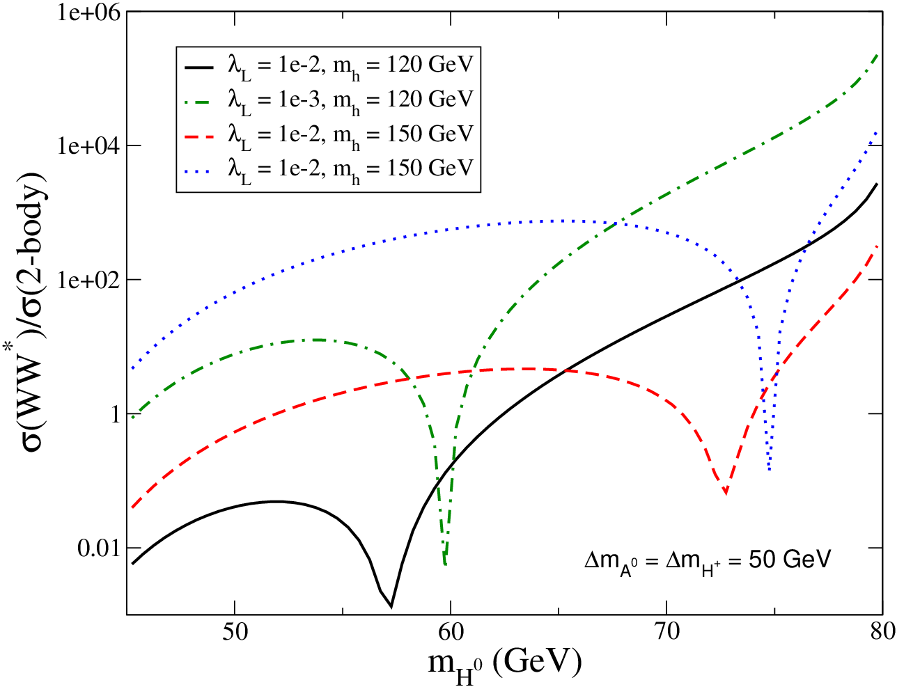
Figure 3 displays the ratio of cross sections as a function of for different values of the higgs mass. For this figure was set to whereas and , which hardly affect the results, were set to . From the figure we see that, the ratio is larger for over the whole range of . For that higgs mass, the ratio increases with and it is larger than in the entire range , implying a dominance of the three-body final state over the two-body ones. For the other two higgs masses, we see that the ratio tends to increase with but it features a narrow dip before reaching the higgs resonance. For the three-body final state dominates the cross section for whereas for it dominates it over the range except for a small mass range around . Independently of the higgs mass, the ratio can be larger than close to the threshold, indicating a strong dominance of the three-body final states in that region.

The annihilation cross section into is affected by via the higgs mediated diagram. This dependence is illustrated in figure 4, which shows as a function of , the ratio of cross sections for two different values of ( and ) and two different higgs masses ( and ). As expected, a smaller suppresses the two-body cross section, which being higgs mediated is proportional to , increasing the relevance of the three-body final state. In fact, the ratio is about two orders of magnitude larger for than for . As a result, for the three-body cross section is larger than the two body one essentially over the entire range we consider, and the ratio can reach values above close to the threshold. Another feature observed in the figure is the displacement of the position of the dip, which due to the smaller interference effects moves closer to the resonance for smaller values of –see appendix B.
As already shown in figure 2, the three-body cross section depends also on the sign of , due to the interference between the higgs mediated amplitude, which goes like , and the other two contributions. Figure 5 shows the ratio of cross sections as a function of for the two possible signs of and two different higgs masses: , . The other parameters were taken as , . The sign of clearly influences the three-body cross section, particularly around the higgs resonance, where the interference is stronger. Notice that the dip moves across the resonance when changes sign. Moreover, the curves for and cross each other exactly at the resonance, as expected. Indeed at that point, the annihilation cross section is entirely determined by the higgs mediated diagram, so there. Notice that the ratio is larger for than for above the resonance, whereas it is the other way around below the resonance. Thus, the largest effect will be obtained for if but for if .
This detailed study of clearly demonstrates that the relevance of the annihilation into the three-body final state is a generic feature of the inert doublet model. No fine-tuning is necessary to find large effects. In the next section we investigate the implications of this new process on the calculation of the inert higgs relic density.
5 Effects on the relic density
To compute the dark matter relic density, one must solve the following Boltzmann equation,
| (4) |
where is the dark matter abundance, defined as the number density divided by the entropy density, is an effective number of degrees of freedom, is the Planck mass, and is the equilibrium thermal abundance. is the thermally averaged annihilation cross section, which must include all relevant annihilation and coannihilation processes. It corresponds to
| (5) |
where run over all annihilating and coannihilating particles, is the number of degrees of freedom of particle , is its mass, is the momentum of the incoming particles in the center of mass frame, and is the total annihilation cross section of particles into Standard Model particles . Integrating equation (4) down to today’s temperature leads to the present dark matter abundance, . From it, the relic density can be obtained as
| (6) |
where is the dark matter particle mass. This standard approach for the calculation of the relic density has been implemented in publicly available software such as DarkSUSY[24, 25] and micrOMEGAs[26, 27, 28, 29].
To properly compute the inert higgs relic density we need to include in equation (5), in addition to the usual two-body annihilation and coannihilation processes, the annihilation into the three-body final state . That is the only modification we need to make to the above procedure –equations (4) and (6) remain the same. For our calculations, we have used a modified version of micrOMEGAs, in which we incorporated the annihilation into the three-body final state in the evaluation of (5). That way, we can accurately compute the relic density of inert higgs dark matter including 3-body final states.
In the following we compare the relic density obtained for two-body final states only (denoted as ) with that predicted including also the final state (denoted as and referred to as the 3-body relic density) for different values of the parameters of the inert doublet model.
 |
 |
Figure 6 shows the relic density derived including only 2-body processes (denoted 2-body) and including 2-body and 3-body processes relic density (denoted 3-body) as a function of for the two possible signs of and two different higgs masses: (left panel) and (right panel). The remaining parameters were taken as , . First of all, notice that the two-body relic density (solid and dotted lines) depends weakly on the sign of , and only for close to . This behavior is to be expected as it is the annihilation into (both being real particles) that brings such a dependence into play, and it is only for close to that such annihilation can take place in the early Universe. The 3-body relic density is observed to be always equal or smaller than the two-body one –as anticipated– and to depend on the sign of . For (left panel) the effect of the 3-body relic density is significant above the resonance, and the predicted relic density is smaller for (dash-dotted line) than for (dashed line). For close to , the dark matter particles may have enough kinetic energy in the early Universe to annihilate into ; consequently, the effect of the three-body final state becomes less relevant in that region. For (right panel), the 3-body relic density is significantly smaller than the two-body one over the entire mass range we consider. Regarding the sign of , both signs give approximately the same relic density below the resonance and differ from each other above it. These two figures demonstrate that the three-body final state affects in a relevant way the predicted relic density of inert higgs dark matter.

To better illustrate the effect of the three-body final state, we next study the ratio between the three-body and the two-body relic density for different sets of parameters. Figure 7 shows this ratio as a function of for different values of the higgs mass. A ratio equal to means that the three-body process gives a negligible correction to the calculation of the relic density. Clearly, that is not the case. The ratio tends to for close to , where the annihilation into is efficient, and for , where the three-body annihilation is suppressed, but in the intermediate region the three-body final state plays a major role, giving rise to a correct relic density significantly smaller than the two-body one. An effect that, as observed in the figure, is present independently of the higgs mass –although its precise magnitude will certainly depend on . Notice, from figure 7, that the two-body approximation may overestimate the predicted relic density by more than one order of magnitude. Moreover, a significant deviation from the two-body result can take place over a wide range of ; depending on the higgs mass, it could extend more than GeV below .

The mass of the CP-odd scalar, , may affect the relic density via coannihilation processes. If the mass splitting between and , , is small, the process increases the annihilation rate and help reduce the relic density. Let us point out that, in the inert doublet model, there is no need to consider possible coannihilations into three-body final states because the two-body ones, being gauge processes, are unsuppressed. Since coannihilations increase the annihilation rate, they are expected to reduce the importance of the three-body final state. That is exactly what is seen in Figure 8, which shows the effect of a smaller on the relic density. It displays the ratio between the 3-body and the 2-body relic density for two values of and two different higgs masses. When , coannihilations are important (dotted- and dashed-lines), and the three-body final state is less relevant –the ratio is closer to – than for when coannihilations are suppressed (solid- and dashed-dotted lines). For the deviation due to the different values of is significant for below whereas for it is so for between and . Notice also that close to the higgs resonance, the annihilation rate is enhanced, making coannihilation effects negligible. That is why the curves for and coincide in the region . Although coannihilation effects slightly reduce its relevance, the effect of the three-body final state remains significant over the parameter space of the inert doublet model.
6 The genuine viable parameter space
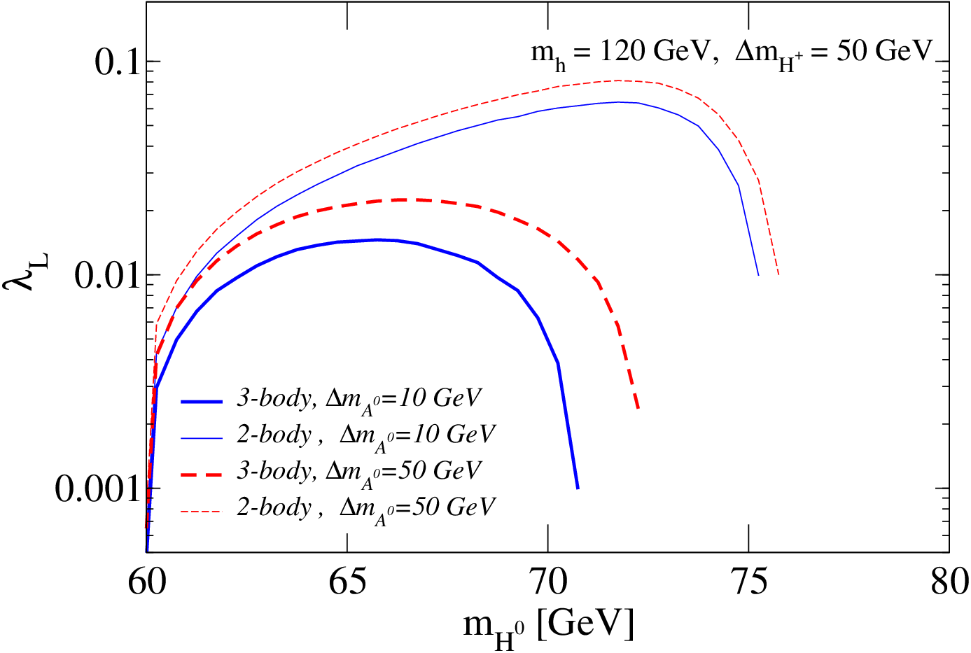
Instead of computing the dark matter density for a given set of parameters, we are usually interested in using the relic density as a constraint on the parameter space of the model. The viable parameter space is determined by requiring that the predicted relic abundance be compatible with the observed density of dark matter [1]. For the inert doublet model, this viable parameter space had been obtained in previous works, but using the two-body relic density, which, as shown in the previous section, is not a good approximation in the intermediate mass regime. In this section, the genuine viable parameter space of the inert doublet model, obtained by including the three-body annihilation into the computation of the relic density, is derived. We study in detail its dependence on the parameters of the model and we demonstrate that it is significantly different from that found for two-body annihilations.
For definiteness, we focus on the following three interesting cases: with , with , and with . Figure 9 shows the viable parameter space of the intermediate mass range of the inert dark matter model in the plane () for GeV, GeV, and two different values of , GeV and GeV. These two values of are chosen so as to indicate the possible effect of having () or not () significant coannihilation processes. The thin lines in this figure correspond to the viable regions if only two-body final states are considered. The thick lines, on the contrary, correspond to the genuine viable regions, those obtained by taking into account two- and three-body final states in the calculation of the relic density. Two important results are clearly observed in this figure. First, the value of for a given mass may be substantially smaller once three-body final states are taken into account. The difference between the two associated to a fixed value of and could amount to one order of magnitude. Second, the viable parameter space shrinks toward lower masses. When only two-body final states are considered, the maximum values of allowed are about and GeV respectively for and GeV. Once the three-body final state is included, the maximum moves respectively to about GeV and GeV. This reduction of the viable mass range is entirely due to the effectiveness of the three-body annihilation, which drives the relic density below the WMAP bound for . In that region, no value of is allowed, for it is the direct annihilation (figure 1, left diagram), a gauge process independent of , that determines the relic density. As observed in this figure, the difference between the two-body and the three-body viable parameter space is quite significant, independently of possible coannihilation effects.
 |
 |
Similar results are found for other higgs masses, as illustrated in figure 10 for (left panel) and (right panel). In both cases was considered and the conventions used were the same as in figure 9. As a consequence of the three-body final state contribution to the annihilation rate of inert higgs dark matter, the required value of is smaller at any given mass, and the maximum allowed value of gets reduced by several s.
Figures 9 and 10 confirm that the modification of the viable parameter space, induced by the annihilation into the three-body final state , is a generic feature of the inert doublet model. A feature that is present over a wide range of independently of the other parameters of the model. It is precisely because of this generality that the intermediate mass regime of the inert doublet model must be revisited, as we do in this paper, in view of these new processes.
These modifications to the viable parameters space are of crucial relevance because they affect other phenomenological aspects of the model. In fact, the first step in the analysis of a given dark matter model is usually the determination of its viable parameter space. Once it is obtained, one can study the specific signatures or predictions of the model within such viable regions. If these are changed so are its predictions and signatures. In the next section we show that, as a result of the new viable parameter space, the direct detection cross section of inert higgs dark matter is considerably reduced.
7 Direct detection of inert higgs dark matter

Dark matter can be detected via elastic scattering with terrestrial detectors, the so-called direct detection method. From a particle physics point of view, the quantity that determines the direct detection rate of a dark matter particle is the dark matter-nucleon scattering cross section. In the inert higgs model, the scattering process relevant for direct detection is higgs-mediated, with a cross section, , given by
| (7) |
where is the reduced mass of the system, is the nucleon mass that we took equal to the proton mass, and is the nucleon form factor, taken equal to for the subsequent analysis (see e.g. the discussion in [11]). Hence, is proportional to . Given the new allowed values of that were derived in the previous section, we foresee that will be significantly reduced with respect to the two-body result used, until now, in the literature.
 |
 |
Figure 11 shows the prediction for along the viable lines of the inert doublet model for . As before, thin lines correspond to the two-body result while thick lines to the three-body one. For comparison, in this figure we also show, as a dotted line, the current limit from CDMS [30]. Notice from the figure that the correct direct detection cross section can be more than two orders of magnitude smaller than the one obtained for two-body final states. In particular, for the genuine direct detection cross section turns out to be well below present bounds.
Analogous results follow also for other values of the higgs mass. Figure 12 shows the same cross section but for (left panel) and (right panel). In both we observe that, over a wide range of , the correct cross section (denoted by 3-body) is significantly smaller than the one derived after including only 2-body processes in the computation of the relic abundance (denoted by 2-body). Notice, for instance, that for the region above the CDMS bound moves from to when the three-body final state is taken into account.
The inclusion of three-body final states is, therefore, mandatory if one wants to make meaningful predictions on the prospects for the direct detection of inert higgs dark matter.
8 Other implications
In this section we briefly address other possible implications of the three-body process on the phenomenology of the inert doublet model. Specifically, we show, in section 8.1, that the annihilation branching ratios can be dominated by the three-body final state, with important implications for the indirect detection of dark matter, and we discuss, in section 8.2, the modifications to the decay width of the higgs boson.
8.1 Indirect detection

The indirect detection signals of inert higgs dark matter are also altered by the existence of the three-body final state . On the one hand, these signals should be now computed along new regions, due to the modified viable parameter space. On the other hand, in these new regions the annihilation cross section and branching ratios typically receive large corrections from the three-body final state . Indeed, we already saw, in section 4, that the annihilation of inert higgs dark matter may be dominated by three-body final states, rather than by the two-body final states considered in previous works. As a result, the spectrum of photons, neutrinos, positrons and antiprotons expected from inert higgs annihilation will be different, changing its indirect detection prospects. Even the gamma ray lines from the one-loop annihilation into two photons [8] will be affected by these new contributions. A detailed study of the implications of three-body final states for the indirect detection of inert higgs dark matter is beyond the scope of the present paper. Here, we just want to demonstrate that, contrary to what has been assumed in earlier analysis on indirect detection of inert higgs dark matter [10], is not necessarily the dominant annihilation channel for . The three-body final state turns out to be dominant over a sizeable region of the viable parameter space.
Figure 13 shows the annihilation branching ratio into the three-body final state as a function of along the viable regions of the inert doublet model. Each line corresponds to a given value of and a given sign of . For this figure we set but the results are similar for other allowed values. Notice that the branching into is indeed significant: it amounts to more than for independently of the higgs mass. Moreover, it reaches values close to for if and also for independently of the higgs mass. In view of these results, the indirect detection signatures of inert higgs dark matter will have to be revised. In a future work, we plan to carry out such an analysis.
8.2 Higgs decays

In the inert doublet model, the higgs boson can decay also into and , increasing the higgs decay width and modifying its branching ratios. A result that is of great interest for higgs searches at colliders [9]. Here we simply illustrate how the higgs decay width is modified when including the three-body final state in the determination of the relic abundance. As before, we assume that accounts for the dark matter of the Universe.
The contribution to the higgs decay with from the decay into the inert scalars is proportional to , so it will be affected by the three-body final state via the new viable parameter space. Figure 14 shows, as a function of , the ratio between the higgs decay width in the inert doublet model and that in the Standard Model, , for . Obviously, the higgs width is only affected for below . For the inert doublet model we consider the result with and without11 1 Notice that and includes the channel in all the curves taking into account the three-body final state in the calculation of the relic density, and we set , . First of all, notice that the higgs decay width can indeed be much larger than what is predicted by the Standard Model. Second, the higgs width in the IDM is slightly smaller once three-body final states are taken into account –see, for instance, the difference between the solid and dotted line or between the dash-dotted and the dashed line. Notice, however, that the region where the deviation from the standard model result is significant, for , is partially excluded by the present direct detection bound from CDMS –see figure 12. This result emphasizes the importance of doing a consistent analysis of the inert doublet model, one that simultaneously takes into account all the relevant effects and the different constraints that can be imposed on the model.
9 Conclusions
We studied the impact, on the phenomenology of the inert doublet model, of dark matter annihilation into the three-body final state . After analyzing its dependence on the parameters of the model, the annihilation cross section into , , was shown to dominate the total dark matter annihilation cross section over a relevant portion of the parameter space. In consequence, the predicted relic density differs considerably from that found in earlier works. We examined in detail the dependence of the inert higgs relic density on the higgs mass and on , as well as the possible role of coannihilations. The genuine viable parameter space of the inert doublet model was derived for different values of the higgs mass and of , emphasizing the differences with respect to the two-body results. We also investigated the direct detection cross section of inert higgs dark matter and found that it can be more than two orders of magnitude smaller than what is predicted without including the three-body final state. Finally, we briefly consider some implications of these new annihilation processes on the decay width of the higgs boson and on the indirect detection of inert higgs dark matter. Summarizing, the inclusion of the three-body annihilation is mandatory, as it strongly affects the entire phenomenology of the inert doublet model.
Acknowledgments
L. L. H was partially supported by CICYT through the project FPA2009-09017, by CAM through the project HEPHACOS, P-ESP-00346, by the PAU (Physics of the accelerating universe) Consolider Ingenio 2010, by the F.N.R.S. and the I.I.S.N.. C. E. Y. is supported by the Juan de la Cierva program of the MICINN of Spain. He acknowledges additional support from the MICINN Consolider-Ingenio 2010 Programme under grant MULTIDARK CSD2009-00064, from the MCIINN under Proyecto Nacional FPA2009-08958, and from the CAM under grant HEPHACOS S2009/ESP-1473.
Appendix A Analytical formula for in the inert doublet model
Here we provide the total amplitude squared for the process , which has been directly obtained with the Calchep package [31]. The relevant Feynman diagrams are shown in figure 1. We denote by the amplitude for the direct annihilation diagram (left diagram in figure 1) and by the higgs mediated diagram (right diagram). correspond to the mediated diagrams (middle). In the following, and denotes the 4-momentum of the annihilating , and are the momentum of the 2 fermions produced in the decay of the virtual and is the momentum of the real .
| (8) | |||||
| (11) | |||||
| (13) | |||||
| (15) | |||||
| (17) | |||||
| (21) | |||||
| (23) | |||||
| (26) | |||||
| (28) | |||||
| (38) | |||||
| (40) | |||||
| (51) | |||||
| (53) | |||||
| (57) | |||||
| (59) | |||||
| (63) | |||||
| (65) | |||||
| (69) | |||||
The cross section can then be obtained, from the total amplitude, in the usual way.
Appendix B Interference effects around the higgs resonance
Around the higgs resonance, cancellations between different contributions clearly appear in . They take place at for and at for . This fact can be easily understood by looking at the square of the sum of the two relevant amplitudes, which are the one of the point like diagram and the one of the higgs mediated diagrams . They can be written as
| (71) | |||||
| (72) |
where, in a similar way to [16], we have defined as the wave function of the outgoing real and as the contribution from the virtual gauge boson and the two outgoing fermions:
| (73) |
For the square of their sum we obtain
| (74) |
Since at low velocities, a negative interference between the two terms should occur for if and for if . That explains why the 3-body annihilation cross section is larger for than for if but it is the other way around for . Moreover, a cancellation between these two contributions takes place at . For GeV and , that position correspond to GeV, in good agreement with figures 3, 4 and 5, which were obtained integrating numerically the cross section including all the contributions displayed in appendix A.
References
- [1] E. Komatsu et al. Five-Year Wilkinson Microwave Anisotropy Probe (WMAP 1 ) Observations:Cosmological Interpretation. Astrophys. J. Suppl., 180:330–376, 2009, 0803.0547.
- [2] Nilendra G. Deshpande and Ernest Ma. Pattern of Symmetry Breaking with Two Higgs Doublets. Phys. Rev., D18:2574, 1978.
- [3] Ernest Ma. Verifiable radiative seesaw mechanism of neutrino mass and dark matter. Phys. Rev., D73:077301, 2006, hep-ph/0601225.
- [4] Riccardo Barbieri, Lawrence J. Hall, and Vyacheslav S. Rychkov. Improved naturalness with a heavy Higgs: An alternative road to LHC physics. Phys. Rev., D74:015007, 2006, hep-ph/0603188.
- [5] Debasish Majumdar and Ambar Ghosal. Dark Matter candidate in a Heavy Higgs Model - Direct Detection Rates. Mod. Phys. Lett., A23:2011–2022, 2008, hep-ph/0607067.
- [6] Thomas Hambye and Michel H. G. Tytgat. Electroweak Symmetry Breaking induced by Dark Matter. Phys. Lett., B659:651–655, 2008, 0707.0633.
- [7] Laura Lopez Honorez, Emmanuel Nezri, Josep F. Oliver, and Michel H. G. Tytgat. The inert doublet model: An archetype for dark matter. JCAP, 0702:028, 2007, hep-ph/0612275.
- [8] Michael Gustafsson, Erik Lundstrom, Lars Bergstrom, and Joakim Edsjo. Significant gamma lines from inert Higgs dark matter. Phys. Rev. Lett., 99:041301, 2007, astro-ph/0703512.
- [9] Qing-Hong Cao, Ernest Ma, and G. Rajasekaran. Observing the Dark Scalar Doublet and its Impact on the Standard-Model Higgs Boson at Colliders. Phys. Rev., D76:095011, 2007, 0708.2939.
- [10] Prateek Agrawal, Ethan M. Dolle, and Christopher A. Krenke. Signals of Inert Doublet Dark Matter in Neutrino Telescopes. 2008, 0811.1798.
- [11] Sarah Andreas, Thomas Hambye, and Michel H. G. Tytgat. WIMP dark matter, Higgs exchange and DAMA. JCAP, 0810:034, 2008, 0808.0255.
- [12] Erik Lundstrom, Michael Gustafsson, and Joakim Edsjo. The Inert Doublet Model and LEP II Limits. Phys. Rev., D79:035013, 2009, 0810.3924.
- [13] Emmanuel Nezri, Michel H. G. Tytgat, and Gilles Vertongen. Positrons and antiprotons from inert doublet model dark matter. JCAP, 0904:014, 2009, 0901.2556.
- [14] Ethan Dolle, Xinyu Miao, Shufang Su, and Brooks Thomas. Dilepton Signals in the Inert Doublet Model. Phys. Rev., D81:035003, 2010, 0909.3094.
- [15] Carlos E. Yaguna. Large contributions to dark matter annihilation from three-body final states. Phys. Rev., D81:075024, 2010, 1003.2730.
- [16] Xue-lei Chen and Marc Kamionkowski. Three-body annihilation of neutralinos below two-body thresholds. JHEP, 07:001, 1998, hep-ph/9805383.
- [17] Yutaka Hosotani, Pyungwon Ko, and Minoru Tanaka. Stable Higgs Bosons as Cold Dark Matter. Phys. Lett., B680:179–183, 2009, 0908.0212.
- [18] Claude Amsler et al. Review of particle physics. Phys. Lett., B667:1, 2008.
- [19] Aaron Pierce and Jesse Thaler. Natural dark matter from an unnatural Higgs boson and new colored particles at the TeV scale. JHEP, 08:026, 2007, hep-ph/0703056.
- [20] G. Abbiendi et al. Search for chargino and neutralino production at s**(1/2) = 192-GeV to 209-GeV at LEP. Eur. Phys. J., C35:1–20, 2004, hep-ex/0401026.
- [21] Sarah Andreas, Michel H. G. Tytgat, and Quentin Swillens. Neutrinos from Inert Doublet Dark Matter. 2009, 0901.1750.
- [22] Marco Cirelli, Nicolao Fornengo, and Alessandro Strumia. Minimal dark matter. Nucl. Phys., B753:178–194, 2006, hep-ph/0512090.
- [23] T. Hambye, F. S. Ling, L. Lopez Honorez, and J. Rocher. Scalar Multiplet Dark Matter. JHEP, 07:090, 2009, 0903.4010.
- [24] P. Gondolo et al. DarkSUSY: Computing supersymmetric dark matter properties numerically. JCAP, 0407:008, 2004, astro-ph/0406204.
- [25] http://www.physto.se/ edsjo/darksusy/.
- [26] G. Belanger, F. Boudjema, A. Pukhov, and A. Semenov. Dark matter direct detection rate in a generic model with micrOMEGAs2.1. Comput. Phys. Commun., 180:747–767, 2009, 0803.2360.
- [27] G. Belanger, F. Boudjema, A. Pukhov, and A. Semenov. micrOMEGAs2.0: A program to calculate the relic density of dark matter in a generic model. Comput. Phys. Commun., 176:367–382, 2007, hep-ph/0607059.
- [28] G. Belanger, F. Boudjema, A. Pukhov, and A. Semenov. micrOMEGAs: Version 1.3. Comput. Phys. Commun., 174:577–604, 2006, hep-ph/0405253.
- [29] G. Belanger, F. Boudjema, A. Pukhov, and A. Semenov. micrOMEGAs: A program for calculating the relic density in the MSSM. Comput. Phys. Commun., 149:103–120, 2002, hep-ph/0112278.
- [30] Z. Ahmed et al. Results from the Final Exposure of the CDMS II Experiment. 2009, 0912.3592.
- [31] http://theory.sinp.msu.ru/ pukhov/calchep.html.