Random graph states, maximal flow
and Fuss-Catalan distributions
Benoît Collins1,2, Ion Nechita1 and Karol Życzkowski 3,4
1Department of Mathematics and Statistics, University of Ottawa, ON K1N8M2, Canada
2CNRS, Université Claude Bernard Lyon 1, Institut Camille Jordan, France.
3Institute of Physics, Jagiellonian University, ul. Reymonta 4, 30-059 Kraków, Poland
4Center for Theoretical Physics, PAS, Al. Lotników 32/44, 02-668 Warszawa, Poland
Abstract
For any graph consisting of vertices and edges we construct an ensemble of random pure quantum states which describe a system composed of subsystems. Each edge of the graph represents a bi-partite, maximally entangled state. Each vertex represents a random unitary matrix generated according to the Haar measure, which describes the coupling between subsystems. Dividing all subsystems into two parts, one may study entanglement with respect to this partition. A general technique to derive an expression for the average entanglement entropy of random pure states associated to a given graph is presented. Our technique relies on Weingarten calculus and flow problems. We analyze statistical properties of spectra of such random density matrices and show for which cases they are described by the free Poissonian (Marchenko-Pastur) distribution. We derive a discrete family of generalized, Fuss-Catalan distributions and explicitly construct graphs which lead to ensembles of random states characterized by these novel distributions of eigenvalues.
1 Introduction
The phenomenon of quantum entanglement in physical systems remains a subject of considerable scientific interest. The case of entanglement in bi-partite systems is relatively well understood [1], but the case of systems consisting of several subsystems is much more demanding and complicated. For instance, the measures characterizing quantitatively quantum entanglement worked out for the simplest case of two subsystems [2, 3] are often not capable to describe the complexity of multi-partite entanglement. On the other hand, the measures applicable in this case, like the geometric measure of entanglement [4] related to the minimal distance of the analyzed pure state to the set of separable states, are in general not easy to compute.
Not being in position to characterize entanglement of a concrete state of a composed quantum system, one often tries to describe properties of a ‘generic’ quantum state. To this end one constructs ensembles of quantum states and computes interesting quantities averaged over the entire ensemble.
In the simplest case of a system consisting of two subsystems one considers an ensemble of random pure states distributed uniformly with respect to the natural, unitarily invariant (Fubini-Study) measure. Quantum entanglement with respect to the partition into these subsystems called and can be described by its entanglement entropy, . Here denotes the von Neumann entropy of the state obtained by the partial trace of the state . As the initial state is pure, the resulting entropy does not depend on the subsystem, with respect to which the partial trace is taken. The entropy is bounded from above by the log of the smaller dimensionality, , where . If this bound is saturated, the initial pure state is called maximally entangled.
The mean entanglement entropy , averaged over the ensemble of random pure states depends only on the dimensionality of both subsystems. An explicit formula for the mean entropy of a subsystem was first conjectured by Page [5] and later proved in [6]. Due to the measure concentration phenomenon the entanglement entropy of a generic pure state is close to the mean value . Concrete bounds relying on the Levy’s lemma [7] specify the probability to find a random state with entropy of entanglement smaller than by .
Note that the Fubini-Study measure on the space of pure states of the entire system followed by the partial trace over subsystem induces a probability measure in the space of mixed quantum states describing the subsystem . These induced measures [8, 9] are parameterized by the dimensionality of the auxiliary subsystem .
Analyzing an ensemble of the reduced random states , Page derived the probability distribution for its eigenvalues. Up to an overall normalization constant this problem is equivalent to finding the density of the spectrum of the Wishart matrices (where is a rectangular complex random matrix of the Ginibre ensemble) studied earlier by Marchenko and Pastur [10]. This very distribution depending only on the ratio of dimensions of both subsystems, is also called free Poissonian, as it corresponds to the free convolution of random matrices [11, 12].
In the general case of pure random quantum states describing multipartite systems one usually studies entanglement with respect to various cuts of the entire system into two parts [13, 14, 15], so the standard measures of the bi-partite entanglement can be applied. Statistical properties of random pure states change if one breaks the overall unitary invariance, characteristic to the Fubini-Study measure, and introduces some structure into the multi-partite system. In particular, for certain numbers of subsystems there exist perfect maximally multipartite entangled states (MMES), such that they are maximally entangled with respect to any bi-partition [14, 16].
Random quantum states are useful to tackle various problems of theoretical physics. A key conjecture of the theory of quantum information processing concerning the additivity of minimal output entropy was recently shown to be false [17, 18]. It is worth to emphasize that the original reasoning was not constructive but it was based on relations between the average quantities computed with respect to an ensemble of quantum states. Entanglement between random states is also interesting in systems motivated by condensed matter physics [19, 20]. For a discussion of a relationship between quantum criticality, Anderson transition and the average entanglement entropy see the recent review [21] and references therein.
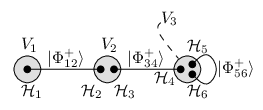
The theory of random pure states proved to be useful to analyze the information flow and the entropy of black holes. The model of Page [22] consisted of two subsystems, the dimensions of which served as parameters of the model. In later models one studied pure states of a system composed of four parties [23, 24]. The system contains two pairs of maximally entangled states which relate subsystems and respectively. The subsystems and are directly coupled together, and the action of an unknown Hamiltonian is mimicked by a random unitary matrix distributed according to the Haar measure. Such a system can symbolically be depicted by a graph containing two edges, which represent two maximally entangled states and a vertex denoting a random unitary matrix. This very situation is shown in Fig. 3b, where a slightly different notation is used.
The main aim of this paper is to extend this construction for an arbitrary (undirected) graph and to investigate properties of the resulting ensembles of multi-partite random quantum pure states. Any graph with edges will be associated with a quantum system consisting of subsystems. Each edge corresponds to a maximally entangled state while each vertex represents a random unitary matrix. The dimensions of two subsystems linked by a given edge of the graph are assumed to be equal, but besides this constraint the dimensions of all the subspaces can be treated as free parameters of the model. As the physical interaction is modeled by a set of random unitary matrices each graph defines an entire ensemble, we call them random graphs states.
Note that such an ensemble of quantum random states associated with a given graph differs form the deterministic construction of graph states introduced by Hein et al. [25]. Furthermore, our approach is not related to quantum graphs reviewed by Gnutzmann and Smilansky [27], which describe quantum particles (or waves) traveling along a graph. A graphic representation of ensembles of random states analyzed in this work looks slightly similar to the one used to define the Projected Entangled Pair States (PEPS) formalism, capable to describe complex many-body systems [28, 29]. While in the latter setup the subsystems entangled with auxiliary systems are coupled together by a projection on a low dimensional subspace, in our approach such a coupling is described by a random unitary matrix.
Any graph defines the topology of couplings between the physical subsystems. Choosing a certain set of the subsystems one can average the pure quantum state over the remaining subsystems. Technically one performs the partial trace the auxiliary subsystems, which leads to a reduced state which generically is not pure. Hence selecting a concrete graph and specifying the subsystems pertaining to the environment we define an ensemble of random mixed states.
In this work we develop general techniques suitable to describe spectral properties of random density matrices associated with a graph. Our technique relies on Weingarten calculus [30, 31], and the observation that its asymptotics boil down to a min-flow problem [32]. In the asymptotic limit, as the dimension of the quantum states goes to infinity, statistical properties the spectrum of a random state can be established, so explicit formulae for its purity and entropy are derived.
We identify these ensembles of random states for which spectra are described by the free Poisson (Marchenko-Pastur) distribution. In some other cases the spectra are described by a discrete family of probability distributions , which can be be considered as generalizations of the free Poissonian distribution. We call them Fuss- Catalan distributions (FC), since their moments are related to the Fuss-Catalan numbers, known in the combinatorics and free probability calculus [33, 34].
The Fuss-Catalan probability distributions are also closely related with properties of products of non-hermitian random matrices. In general, products of random matrices are often studied in context of various problems of statistical physics [35]. Recent studies on products of Ginibre matrices concern multiplicative diffusion processes [36], rectangular correlation matrices used in macroeconomic time series [37] and lattice gauge field theories [38]. Spectral properties of a product of random Ginibre matrices were analyzed in a recent paper of by Burda et al. [39].
In the simplest case random matrices described by the distribution have the structure where and are independent random Ginibre matrices. In the general case of an arbitrary integer the random states are proportional to the Wishart matrix , constructed out of a product of independent Ginibre matrices, .
To analyze statistical properties of random states whose definition is based on random unitary matrices, one needs to perform averages over the group of unitary matrices. Instead of using explicit formulae derived by Mello [40] we found it more convenient to use the Weingarten calculus (see e.g. [30, 41]). In order to evaluate expectation values for random tensors we are going to use a diagramatic approach and a graphical calculus recently developed in [31].
This paper is organized as follows: ensembles of pure states corresponding to classical graphs are defined in section 2. In section 3, we discuss mixed states which arise by taking the partial trace over a specified set of subsystems. In section 4 graphical and combinatorial tools used to perform integration over the unitary group are described. The main result of this work — a general technique to compute the moments of the spectrum of ensembles of mixed states obtained by partial trace — is presented in section 5. In section 6 we analyze ensembles associated to some particular graphs (star graphs, cycle graphs) and find ensembles of mixed states characterized by Marchenko-Pastur and Fuss-Catalan distributions. Some other graphs which lead to other, “exotic” distributions are also provided. The paper is concluded in section 7 in which we summarize results obtained and present a list of open questions.
2 Classical graphs, quantum pure states and random matrices
In this section we describe a family of quantum pure states that are associated in a natural way with undirected graphs. The underlying idea is that vertices of graphs correspond to quantum systems and edges describe the entanglement between the systems. A particular feature of the states we consider is that the entanglement described by the edges will be maximal.
Consider an undirected graph consisting of edges (or bonds) and vertices . We allow multiple edges between two vertices, as well as vertex loops. Note that the graphs considered here are not metric, so we do not discuss the lengths of the edges. Let denote the degree of the vertex defined as the number of edges attached to this vertex (each loop counts twice). As an example, for the graph in Figure 1, we have , , .
We are going to analyze quantum states belonging to the Hilbert space with the -fold tensor product structure, . The dimension of the subspace is , where the parameters are fixed while the number is arbitrary and we will eventually discuss the limit . The total dimension of space reads thus .
A graph with edges induces a tensor product structure of the -fold tensor product space . The vertices of induce a partition of the set , with blocks . The reader can think about the Hilbert spaces living inside the vertex . For each vertex , we introduce the Hilbert space which describes the subsystems of the vertex .
Each edge of the graph represents the maximally entangled states between two Hilbert spaces and . More precisely, we shall ask that and we put
| (1) |
where and are orthonormal bases for and . The actual choice of the two bases is not important in what follows, but we shall assume that these bases are fixed.
In order to introduce an ensemble of random graph states belonging to we are going to use independent, random matrices , distributed according to the Haar measure. The matrix corresponds to the -th vertex of the graph, . It acts on the space (and thus on subspaces) and describes the coupling at a given vertex. To specify the subspaces coupled by a unitary matrix it will be also convenient to use an alternative notation and write where denotes the degree of the vertex. See Figure 1 for a concrete example of a graph and a graph ensemble.

The simplest graph ensembles described by our model have only one edge. We consider two cases, one where the unique edge is a loop of one vertex, and the second one where the edge connects two vertices (see Figure 2).
In the first situation, the graph has a single vertex of degree two. This graph corresponds to the system consisting of subsystems. The edge represents the maximally entangled state, but due to the global unitary matrix , is a random state in . Since is generated according to the Haar measure, the random state is distributed uniformly with respect to the Fubini-Study measure, as in the model of Page [5], so in this case the bond forming the loop is in a sense redundant.
In the linear case, we have again only one edge, , two vertices, , and each vertex contains only one node. The graph is represented in Figure 2 (c) and (d), both in the simplified and in the standard form. The random quantum pure state associated to this graph is a generic maximally entangled state,
| (2) |
where we set and where represent independent random unitary matrices. Here , denote some fixed bases of .


As a third and final example, the next simplest graph one could imagine has a linear shape, edges, vertices , , and nodes, as in Fig. 3.


In general, any graph is associated with a collection of subspaces , each endowed with some fixed orthonormal basis. We consider two partitions of the set . A pair partition with the property that , represents all bonds in the graph and thus the entangled states. The second partition consists of blocks of size , which represent the vertices of the graph, and encode the random unitary operators . For instance, in the case of subspaces presented in Fig.1 the two partitions read and .
These two partitions allows us to introduce a general definition of an ensemble of graph random states
| (3) |
where are Haar independent random unitaries and are the maximally entangled states (1) defined with respect to the fixed orthonormal bases of and .
3 Marginals of random graph states
To study non-local properties of the random graph state associated to a graph it is useful to specify a partition of the set of all subsystems into two groups, . Then it is possible to treat the multi-partite state as if it where bipartite and to analyze its entanglement with respect to this concrete partition. The entanglement of a bipartite pure state can be measured by the von Neumann entropy of the reduced state obtained from the initial projector by the partial trace. We will analyze the partial trace of the pure state over a subspace defined by the subset of the set . Then denotes the complementary subset, so the sum of their elements is equal to and the entire Hilbert space can be written as a tensor product, . Such a partial trace will be briefly denoted by and the resulting density matrix is supported then by the subspace ,
| (4) |
Graphically, partial traces are denoted at the graph by “crossing” the spaces which are being traced out. For example, in Figure 4, the partition defining the bi-partite structure is . In the diagram, the dots representing the subspace , and are “crossed”, and the partial trace is taken on the tensor product of those spaces .
Before exploring the quantitative entanglement of , we can make some qualitative remarks right away. Looking at Figure 4 we see that the systems and are not entangled before the random unitary transformation was applied. Indeed, before applying the random unitary matrices, the state of the system reads
| (5) |
The product structure of the state is given by the supremum of the vertex and edge partition, . However, after the unitary transformations, subsystems and become entangled (generically); one might say that entanglement was broadcasted by the unitary matrix .
In general, we define the partition by
| (6) |
where denotes the block of and in . In other words, is obtained from in the following way: if a block of is entirely traced out, then replace it by singletons, otherwise keep it as it is. The block structure of is then given by the restriction of the partition to the set . For the graph in Figure 4, we have , , and . Since the unitary is not completely traced out, it is capable to broadcast the entanglement between subsystems and .

We finish this section by a remark which can simplify the structure of graph state marginals in some cases. If a marginal of the pure state (3) is considered, the unitaries corresponding to singletons in equation (3) can be replaced by the identity operator if the pair of in is not a singleton in . This follows from the invariance of the Haar measure on the unitary group and from the fact that one can extract an independent unitary from the block of in .
4 Graphical and combinatorial tools for unitary integration
4.1 Permutations, non-crossing partitions
In this section, we introduce notation that will be used in the entire paper and which may be non-standard. For an integer , let denote a set of elements . For a collection of numbers , Hilbert spaces and for a set of indices , we are going to use the notation and .
We denote by the group of permutations on elements. For a permutation , we call its length, that is the minimum number of transpositions necessary to obtain and the number of disjoint cycles of . One has for all permutations . Note that the absolute value is also used in this work to denote the cardinality of a set .
We consider the lattice of partitions of , and say that if, for any block of there exists a block of that contains , . For any partitions and define (resp. ) to be the least upper bound (resp. the greatest lower bound) of and with respect to the previously defined partial order, and also let (resp. ) the greatest (resp. smallest) element in .
The permutation group admits a natural left action on the partitions of . Call the orbit to which belongs. These orbits are in natural one to one correspondence with the partitions of the integer . For any permutation , we denote by the partition of whose blocks are the orbits of .
The lattice admits a subset of interest, of set of all non-crossing partitions. We denote it by . A partition is called non-crossing iff there exists no two different blocks of the partition and , , with . is a sub-poset of and it turns out to be a lattice as well. The operation is the same for and , however the supremum operation is different in the non-crossing setting, as it can be seen by the example and .
We consider the vector subspace of functions whose value is when does not hold. This vector space is endowed with a convolution operation
| (7) |
This turns into an algebra with unit . For each such that , there exists a partition such that the interval is isomorphic as a lattice to the lattice . If then define the Möbius function by
| (8) |
where
| (9) |
is the -th Catalan number (later we shall see that Catalan numbers are a particular case of a much more general class of combinatorial family, called the Fuss-Catalan family). We also define the Zeta function which is equal to one when and zero otherwise:
| (10) |
In this paper we will need the fact that the convolution product of the Möbius function and the Zeta function is equal to the Kronecker delta function iff. :
| (11) |
Note that if we had considered the equation (7) in the general lattice of partitions and had left the definition of unchanged, we should have modified the definition of as follows.
We finish this section by mentioning the following fact, of crucial importance in what follows: if is a permutation with one cycle (i.e. a cyclic permutation), the set is in one to one correspondence with the set of non-crossing partitions . If , which we can always assume up to an overall conjugation of the set , the correspondence is given by . The proof of this result is elementary and belongs to combinatorial folklore.
4.2 Weingarten calculus
In this section, we recall a few facts about the Weingarten calculus, useful to evaluate averages with respect to the Haar measure on the unitary group.
Definition 4.1.
The unitary Weingarten function is a function of a dimension parameter and of a permutation in the symmetric group . It is the inverse of the function under the convolution for the symmetric group ( denotes the number of cycles of the permutation ).
Notice that the function is invertible for large , as it behaves like as , were denotes the number of elements in the permutation group . We refer to [41] for historical references and further details. We shall use the shorthand notation when the dimension parameter is obvious.
The following theorem relates integrals with respect to the Haar measure on the unitary group and the Weingarten function . (see for example [30]):
Theorem 4.2.
Let be a positive integer and , , , be -tuples of positive integers from . Then
| (12) |
If then
| (13) |
We are interested in the values of the Weingarten function in the limit . The following result encloses all the data we need for our computations about the asymptotics of the function; see [30] for a proof.
Theorem 4.3.
For a permutation , let denote the set of cycles of . Then
| (14) |
and
| (15) |
where is the -th Catalan number.
A shorthand for this theorem is the introduction of a Möbius function on the symmetric group, invariant under conjugation and multiplicative over the cycles, satisfying for any permutation :
| (16) |
where is the length of , i.e. the minimal number of transpositions that multiply to , and was defined at equation (8). We refer to [41] for details about the function .
Next, we recall briefly the results of [31] for the convenience of the reader and in order to make the paper self contained.
4.3 Axioms of unitary graphical calculus
The purpose of the graphical calculus introduced in [31] is to yield an effective method to evaluate the expectation of random tensors with respect to the Haar measure on a unitary group. The tensors under consideration can be constructed from a few elementary tensors such as the Bell state, fixed kets and bras, and random unitary matrices. In graphical language, a tensor corresponds to a box, and an appropriate Hilbertian structure yields a correspondence between boxes and tensors. However, the calculus yielding expectations only relies on diagrammatic operations.
Each box is represented as a rectangle with decorations on its boundary. The decorations are either white or black, and belong to . Figure 5 depicts an example of boxes and diagrams.


It is possible to construct new boxes out of old ones by formal algebraic operations such as sums or products. We call diagram a picture consisting in boxes and wires according to the following rule: a wire may link a white decoration in to its black counterpart in . A diagram can be turned into a box by choosing an orientation and a starting point.
Regarding the Hilbertian structure, wires correspond to tensor contractions. There exists an involution for boxes and diagrams. It is anti-linear and it turns a decoration in into its counterpart in . Our conventions are close to those of [46, 47]. They should be familiar to the reader acquainted with existing graphical calculus of various types (planar algebra theory, Feynman diagrams theory, traced category theory). Our notations are designed to fit well to the problem of computing expectations, as shown in the next section. In Figure 5, 5 and 5 we depict the trace of a matrix, multiplication of tensors and the tensor product operation. For details, we refer to [31].
4.4 Planar expansion
The main application of our calculus is to compute expectation of diagrams where some boxes represent random matrices (e.g. Haar distributed or Gaussian). For this, we need a concept of removal of boxes and . A removal is a way to pair decorations of the and boxes appearing in a diagram. It therefore consists in a pairing of the white decorations of boxes with the white decorations of boxes, together with a pairing between the black decorations of boxes and the black decorations of boxes. Assuming that contains boxes of type and that the boxes (resp. ) are labeled from to , then where are permutations of .
Given a removal , we construct a new diagram associated to , which has the important property that it no longer contains boxes of type or . One starts by erasing the boxes and but keeps the decorations attached to them. Assuming that one has labeled the erased boxes and with integers from , one connects all the (inner parts of the) white decorations of the -th erased box with the corresponding (inner parts of the) white decorations of the -th erased box. In a similar manner, one uses the permutation to connect black decorations.
In [31], we proved the following result:
Theorem 4.4.
The following holds true:
5 Main result: computing the moments of and a flow problem
5.1 A formula for the moments of
This section contains one of the main results of the paper, Theorem 5.1.
We present a general method for computing the moments of the random density matrix obtained by partial tracing a random graph state (4) over the subsystems labeled by . Here denotes a partition of the total number of subspaces. For each block of , we define the sets and . These sets define a partition of each vertex and contain the information on which subsystems of the vertex are being traced out. Let be the set of bonds with both ends in . Additionally, we have to take into account the bounds between the different blocks. For , let . Notice that and that . Since the edges of the graph are not oriented we shall put, for , . Each unitary block is partitioned in two ways: by the partial tracing operation, , and by the type of bonds it contains: .
For the case depicted in Figure 1, the vertex partition is made of 3 blocks: , and . We represent it in Figure 6. For the block for example, one has , , , and .


The marginal we are considering in Figure 6 is . In the diagrammatic picture of [31], the density matrix is represented in Figure 6.
In the general case, the constant in front of the diagram is meant to normalize the Bell states appearing in and it has a value of . Using the graphical Weingarten formula (Theorem 4.4), we obtain the following theorem, which contains the main result of this section.
Theorem 5.1.
The moments of a graph state marginal are given by the exact formula
| (17) |
Proof.
For each independent unitary matrix , counts the contribution of the loops corresponding to partial traces, corresponds to the moment product, corresponds to loops created by Bell states inside and, for each couple , represents the contribution of the loops coming from the Bell states between vertices and . ∎
The Weingarten functions appearing in equation (17) are intractable at fixed dimension . In the following section, we shall investigate the marginals in the asymptotic regime (keeping fixed).
In order to compute the dominating term in equation (17), we look at the exponent of for each term in the sum (we use the first order asymptotic for the Weingarten function (16) and the fact that for all permutations , ):
| (18) |
Using, for all , , and the fact that , we conclude that the general term in equation (17) has the following asymptotic behavior:
| (19) |
where
| (20) |
One has to minimize the function over in order to find the dominating term in equation (17). The following simplification can be made at this point:
Lemma 5.2.
The minimum of the function is the same as the minimum of the function defined by:
| (21) |
Proof.
5.2 The minimization problem on permutations as a maximal flow problem
We will now exhibit a connection between the minimization problems (20) and (21) and a maximum flow problem on a network. For an introduction to the maximum flow on networks, see [32], Chapter 27. We introduce a network with vertex set , edge set and edge capacities . The network is associated to the minimization problem for (21) in the following way. The vertex set is given by , with two distinguished vertices: the source and the sink . The edges in are oriented and they are of three types:
| (22) |
The capacities of the edges are given by:
| (23) |
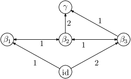
Let us now consider the maximum flow problem on the network , with source and sink . A flow in a network is a function with the following three properties:
- 1.
Capacity constraint: for all vertices , ;
- 2.
Skew symmetry: for all , ;
- 3.
Flow conservation: for all vertices different from the source and the sink ,
(24)
The value of a flow is the quantity
| (25) |
In the maximum flow problem, we want to determine a flow of maximum value in the network . The Ford-Fulkerson algorithm states that solutions to the maximum flow problem are obtained as sums of augmenting paths. One starts with an empty flow . An augmenting path is obtained by pushing a quantity of flow through a path , such that, for all edges of the path, . One can then update the flow function by adding units of flow to each of . The weights are also updated by subtracting from the capacities of the edges above. The new network, with updated capacities, is called the residual network. One iterates this procedure until no more augmenting paths exists. The maximal flow that can be sent from to is denoted by . The final residual network is denoted by . Note that contains only edges for which .
Let us analyze now the connection between a solution of the maximal flow problem and . Each time a flow is sent through a path , we write the triangular inequality
| (26) |
Summing up all this inequalities for the augmenting paths that add up to the maximal flow , we have that
| (27) |
Moreover, we claim that equality can be achieved in . The residual network has the property that it contains no augmenting paths. This means that the source and the sink are in different connected components of the graph . The equality case in is obtained by setting for all permutations in the connected component of the source . Similarly, put for all vertices in the connected component of the sink . Finally, impose that for all permutations lying in a connected component different from the ones containing of . In this manner, all extra terms in equation (27) are zero, and one has indeed .
In conclusion, we have showed that always holds, where is the maximum flow on the network . Of course, does not depend to the solution (i.e. the choice of the augmenting paths leading to the maximum flow) to the maximum flow problem. Moreover, we have showed that for each solution , equality can be attained by choosing permutations in a way depending on the residual network (which depends on the solution ). Let us now describe exactly, for a solution to the maximum flow problem, the set of -tuples which saturate the inequality .
Firstly, each time an augmenting path in is chosen, we use the triangular inequality (26). This implies that all permutations are geodesic permutations (i.e. elements of and that they satisfy
| (28) |
where we note by the cycle partition of a permutation. Actually, since we are dealing with geodesic permutations, it follows (see e.g. the last paragraph of section 4.1), that these partitions are non-crossing. Hence, each augmenting path imposes two conditions on the permutations it contains: they should all be geodesic permutations and their associated non-crossing partitions should satisfy a linear ordering inequality (28). Moreover, the condition that the extra terms in equation (27) should be zero imposes additional constraints on the permutations (except, of course, in the case where is empty, and all connected components of the residual network are singletons). These conditions impose that all permutation lying in the same connected component of should be equal (so that the terms are all null). Hence, the permutations achieving the minimum for , for a solution of the maximum flow problem, should satisfy the following constraints (note that we are referring to the connected components of the final residual network ):
| (29) |
Two important comments should be made at this point. Using the properties of the augmenting flow, it is fairly easy to see that the above system of equations and inequalities is consistent. Moreover, all solutions of (29) are geodesic permutations. We have seen that this already holds for permutations which belong to at least one augmenting path. A permutation not belonging to any augmenting paths is connected in the residual network to either the source or to the sink (but not to both, since in that case will be a valid augmenting path in the final residual network, which is impossible). In that case, or , which are both geodesic permutations.
Let be the set of solutions to (29). It can be described by a poset , endowed with a partial order :
| (30) |
Since there are more than one possible solutions to the maximum flow problem (all having the same value ), the general solution to the minimization problem (21) is given by the union over possibilities:
| (31) |
The solution of the minimization problem for the ’s being settled, let us move now to the initial minimization problem for over , stated in equation (20). We solve the problem completely, by characterizing all the permutations which achieve the minimum. We shall consider three cases for a vertex (which depend only on the initial network):
- (I)
: the vertex is connected to both the source and the sink in the network ;
- (II)
: the vertex is connected only to the source in the network ;
- (III)
: the vertex is connected only to the sink in the network .
Definition 5.3.
A vertex is said to be of type “T” if all the subsystems of are traced out. A vertex is called a type “S” vertex if none of the subsystems of are traced out.
In the first case, when going from the -minimization problem to the -minimization problem, we used both triangle inequalities and at least once. For a fixed vertex and a fixed permutation , the unique solution to the system
| (32) |
is . This follows from the following chain of inequalities:
| (33) |
and hence , for all vertices of type (I).
In the case (II) above, since , only the triangle inequality must be saturated. Hence, for a given geodesic permutation , the set of permutations which saturate the triangle inequality is the geodesic set . In other words, we have to consider all the geodesic permutations such that . By considering all the possibilities for , one needs to compute the sum
| (34) |
Using the fact that the function is related to the Möbius function on the poset of non-crossing partitions, one can show (see [12], chapter 10 and equation (11)) that the above sum is non-zero only if the above sum is trivial, that is, only if . Thus, permutations corresponding to a vertex which is connected only to the source (i.e. a type “T” vertex) must satisfy . Similar ideas lead to the conclusion that all type “S” vertices (case (III) above) need to satisfy . Moreover, we have shown, in all three cases (I)-(III) above, that the permutations which achieve the minimum satisfy , for all . This greatly simplifies equation (20), since the Möbius functions are trivial: .
In conclusion, since some of the solutions in equation (31) cancel out, we define, for each solution of the maximum flow problem, the set
| (35) |
We introduce the modified (smaller) set of general solutions to the minimization problem:
| (36) |
We sum up the preceding discussion in the following theorem, the main result of this section.
Theorem 5.4.
| (37) |
In the simplified situation when the parameters are trivial, , the above theorem admits the following corollary, which provides a simple combinatorial formula for the moments of a graph state marginal. Both combinatorial quantities below (the maximum flow and the cardinality of the set of solutions ) can be computed from the network associated to the marginal.
Theorem 5.5.
Consider a graph state with the property that the relative dimensions of its subsystems are unity (). The average moments of a marginal are given by the simple combinatorial formula
| (38) |
where is the maximum flow associated to the marginal and is determined by the set of augmenting paths corresponding to the maximum flow problem.
Theorem 5.5 is very convenient in the sense that it turns the problem of computing moments into the problem of counting the number of solutions of a maximum flow problem. This is a rather unexpected mathematical connection between quantum physics and networking theory.
Remark 5.6.
When one interchanges the elements of the partition defining the marginal , all the objects in the above discussion are replaced by their duals. In the network, the source and the sink are exchanged; the value of the maximum flow does not change, and all the inequalities for the ’s are reversed. This means that geodesic permutations and are replaced by their Kreweras complement. Hence, the asymptotic moments do not change. This was expected, since the spectra of and differ only by null eigenvalues.
In this paper, we are making heavy use of the Fubin-Study measure. It is the most natural one, as it ensures norm preservation of the states. However it is not the simplest one, and it would be computationally simpler to deal with random Ginibre ensembles instead of unitary matrices. The following observation shows that the results are asymptotically the same:
Remark 5.7.
The graphical calculus that we recalled in section 4.4 has a Gaussian counterpart [45], and it follows by rather direct inspection that the Theorems 5.4 and 5.5 would yield the same asymptotic results if one replaced in our model unitary matrices by (properly normalized) non-hermitian standard complex Gaussian random matrices. Non-hermitian standard complex Gaussian matrices are less natural (and in particular they are not norm preserving). However the graphical calculus is much simpler, as the Weingarten calculus has just to be replaced by Wick theorem (i.e. Feynman diagrams). The reason why one obtains the same result, is that for the Gaussian case, one does not have ’s and ’s but just ’s and one ends up directly with the minimization problem for . The fact that the leading coefficients are the same follows from the non-crossing Möbius inversion formula (11).
We are not able to give physical reasons why the Gaussian and the unitary model have the same asymptotic behavior in general and it seems non-obvious to us without a direct computation of moments.
6 Applications
In the last part of the paper, we study applications of the theory developed in the preceding sections. We start by introducing the Fuss-Catalan probability distributions which appear as limit eigenvalue distributions in some special cases. We then study particular graphs (stars graphs, cycles) and the density matrix ensembles one obtains by partial tracing the corresponding random pure states. Finally, in Section 6.6, we study marginals of graph-states which lead to new probability distributions.
6.1 Free Poisson and Fuss-Catalan distributions
In Random Matrix Theory, the free Poisson (or Marchenko-Pastur) distribution describes asymptotically the spectral density of the normalized random Wishart matrices , where is a random rectangular matrix from the Ginibre ensemble of size . The Marchenko-Pastur distribution is also the limit spectral density of rescaled density matrices from the induced ensemble [26, 43]. If denotes an eigenvalue of a normalized random Wishart density matrix of size the probability density of the variable is asymptotically given by the free Poisson probability measure with parameter ,
| (39) |
where denotes the indicator function of the set .
In free probability theory, this distribution is also called the free distribution, and it has a semigroup structure with respect to the additive free convolution of Voiculescu: (see, e.g. [12]). Moreover, can be characterized by the fact that all its free cumulants are equal to .
The mean purity for the Marchenko-Pastur distribution reads . One can compute the mean entropy of this probability distribution (note that in this work, logarithms are considered in base 2, )
| (40) |
In the case it is equal to , so the mean entropy of a random density matrix of size generated out of a square Ginibre matrix behaves asymptotically () as .
Next, we recall a few facts about a series of probability distributions that was discovered recently in relation to quantum group theory in [34], and which generalize the free Poisson distribution (39). These distributions depend on a real parameter and are most easily characterized by their moments. Four our purposes it is convenient to extend the meaning of the binomial notation: for an arbitrary real number and a natural integer we set
| (41) |
Theorem 6.1.
For any real number , there exists a probability measure , called the Fuss-Catalan distribution of order , whose moments are the generalized Fuss-Catalan numbers (see, e.g. [33]):
| (42) |
The measure has no atoms, it is supported on where , its density is analytic on , and bounded at , with asymptotic behavior at .
This distribution arises in Random Matrix Theory when one studies the product of independent random square Ginibre matrices, . In this case, and squared singular values of (i.e. eigenvalues ) have asymptotic distribution . In terms of free probability theory, it is the free multiplicative convolution product of copies of a Marchenko-Pastur distribution [34]:
| (43) |
One can further generalize Fuss-Catalan distributions in the following way. Consider independent rectangular Ginibre matrices of dimension ratios and such that the product is well defined. The asymptotic level distribution for the (rescaled) eigenvalues of is then . The new, generalized measure depends on parameters which describe the dimension ratios for each matrix. In free probability this corresponds to taking Marchenko-Pastur distributions with different parameters :
| (44) |
In the case of an integer , the Fuss-Catalan numbers count the number of -chains in the lattice of non-crossing partitions [33]:
| (45) |
In [34], the authors interpreted these numbers as the moments of free Bessel laws. They showed that these numbers count non-crossing partitions of into blocks of size multiple of (for a bijective proof of this statement, see [33]):
| (46) |
Using the moment formulas, one can compute the entropy of the Fuss-Catalan distributions.
Proposition 6.2.
The entropy of the Fuss-Catalan measure is given by
| (47) |
Proof.
Using the analyticity of the density, we can write the Shannon entropy as a limit of Rényi entropies, by replacing factorials in the definition of by Gamma functions:
| (48) |
Next, we write the above limit as a logarithmic derivative at of the function
| (49) |
Using the expression of the derivative of Gamma function at integer points
| (50) |
where is the Euler constant, we can conclude. ∎
The second member of the Fuss-Catalan family, corresponds to a product of independent Ginibre matrices. Note that a related analysis of a product of two real random correlation matrices was performed by Bouchaud et al. [37], who used the term Marchenko-Pastur square distribution, and independently by Benaych-Georges [44], who studied multiplicative convolution of free Poisson laws. The formulas in equation (42) for allow to explicitly solve for the density of this measure:
| (51) |
A plot of the density of is given in Figure 8, along with the density of the free Poisson distribution .

6.2 Marginals of graphs leading to Fuss-Catalan distributions
We provide in this section examples of simple graphs and associated marginals whose limit distributions are members of the Fuss-Catalan family of probability laws introduced in the preceding section. The examples chosen here have the property of being the simplest ones which lead to Fuss-Catalan limits.


The simplest case, , corresponds to the free Poisson (or Marchenko-Pastur) distribution. This distribution is the limit of the induced ensemble of random density matrices studied in [43, 26]. The simplest graph having the Marchenko-Pastur distribution as a limit, is the one-loop graph, with one vertex containing two subsystems (or Hilbert spaces) inside. The marginal we consider is the one where we trace out one system, keeping the other (since we assume that all the Hilbert spaces are isomorphic to , the indices of the systems being traced out do not matter). The simple graph, the marginal and the associated network are represented in Figure 9. The maximum flow problem associated to the network is trivial, one unit of flow being sent through the path . The residual network is empty and it follows from Theorem 5.4 that
| (52) |
The number of all non-crossing partitions of is known to be the -th Catalan number , which is also the -th moment of the Marchenko-Pastur distribution . By construction both subsystems are of the same dimension so if one performs partial trace over one of them the resulting mixed state is distributed according to the Hilbert-Schmidt measure [42, 43] and the ratio parameterizing the Marchenko-Pastur distribution reads .
We now move on to the first non-trivial case, . The graph we consider (see Figure 10) has two vertices connected by an edge and each having a loop attached. The marginal of interest is the one obtained by partial tracing two copies of in the first vertex and one copy of in . In the network associated to this marginal, a maximum flow of 3 can be sent from the source to the sink : one unit through each path , and one unit through the path . In this way, the residual network is empty and the only constraint on the geodesic permutations is
| (53) |
i.e. and form a 2-chain in . It follows the moments of the marginal are given by
| (54) |
and thus the rescaled random matrix converges in distribution to the second Fuss-Catalan measure .


The construction for the graph state and its marginal in Figure 10 can be easily generalized to obtain graph state marginals having as a limit distribution. The main idea behind this construction is the structure of the network in Figure 11. The maximum flow in this network is and it can be obtain by sending one unit of flow through the following paths:
| (55) |
The residual network is empty, and thus the combinatorial factor appearing in equation (17) is given by the number of -chains in . In conclusion, the moments of behave asymptotically as
| (56) |
The empirical eigenvalue distribution of the rescaled marginal converges to the Fuss-Catalan distribution .


6.3 One-unitary marginals of general graphs
The next class of examples we shall investigate using the techniques developed in Section 3 is a rather general one. In this section, we consider marginals of graph states with the property that the set of “surviving” subsystems is contained in one block of the vertex partition . Note however that we do not impose any conditions on the underlying graph.
We consider a general graph with nodes and edges. As in Section 2, to such a graph we associate a random pure state on a -fold tensor product. We are interested in a marginal
| (57) |
with the property that is contained in a single block of the partition defining the vertices of . Without loss of generality, we can relabel the Hilbert spaces is such a way that , where is the number of subsystem of the “surviving” vertex.
For a specific example, see Fig. 12, in which . As we shall see, the other nodes of the graph will not play any role in the statistical properties of , so they are not represented in Figure 12.
The single -vertex represents a random unitary matrix , which acts on subspaces labeled by the set of indices in the block . As before, denotes the set of subspaces traced out, so the reduced matrix lives in the complementary subspace . Let the set of vertices in that are being traced out (). We are interested in computing the distribution of the random matrix . Since lives on , the probability distribution of the random density matrix is invariant with respect to any unitary conjugation on .
Lemma 6.3.
The distribution of is -invariant.

Two subsets of play an important role in what follows. The set supporting the reduced density matrix and the set of bonds which are contained in :
| (58) |
In Fig. 12, and . In the graphical notation of [31], the state corresponding to Fig. 12 is represented in Figure 13. The unitary blocks corresponding to vertices which were traced out were removed from the diagram, using the unitary axiom . Using the box-manipulation rules of [31], subsystems in connected to other vertices in the initial graph are linked now by “identity wires” (subsystems in Figure 13). Notice that although the Hilbert spaces with may have different dimensions, we used round-shaped labels for all of them, for obvious practical reasons.
Let the set of bonds complementary to set be denoted by . It consists of nodes which represent bonds connecting nodes of with nodes belonging to other vertices of . In the case shown in Fig. 12 we have . Since the sets and , and respectively and are complementary with respect to , we have

The normalizing constant appearing in the diagram comes from the different normalizations of the input states: for every Bell state associated to an “internal” bond and for every identity matrix corresponding to an index . Putting all these contributions together, we have
| (59) |
The main result of this section is the following theorem, describing the asymptotic behavior of the marginal . We shall provide two proofs of this result: the first proof is direct, and it uses the graphical calculus in [31]. The second one makes use of Theorem 5.4 in Section 5.1.
Theorem 6.4.
For a graph , let be the associated random pure state and consider
| (60) |
a marginal of this random state with the property that is contained in a single block of the partition defining the vertices of . The vertex contains nodes, out of which are connected to other vertices. The partial trace above is taken over subspaces of joint dimension . The reduced density matrix , supported by the complementary subspaces of dimension , is asymptotically () characterized by the following behavior
- (I)
If , the state converges in moments to the maximally mixed state in .
- (II)
If , then the rescaled operator converges in moments to a free Poisson distribution (see equation (39)) of parameter .
- (III)
If , the reduced state has rank . If is the restriction of to its support, then converges in moments to the maximally mixed state in . The support of is a dimensional Haar random subspace of .
Proof.
Using the unitary invariance, it is easy to see that one can replace the tensor products of maximally entangled spaces by any rank-one projector. Using this trick and collecting all the vector spaces corresponding to the sets , , , , one obtains the simplified diagram for depicted in Figure 14.

Following Theorem 5.1, one can compute the moments of the random matrix using the Weingarten function and the graphical calculus:
| (61) |
Since we are interested in the asymptotical regime , we investigate the power of in the sum above:
| (62) |
Using the equality , we find that the exponent of that one wants to maximize in order to obtain the dominating terms is
| (63) |
Using the triangular identities
| (64) | ||||
| (65) |
times and times respectively, we look at the (a priori) weaker minimization problem over
| (66) |
Before solving this minimization problem, let us consider the extremal cases where or . If , then every subsystem of is traced out, and the reduced state is degenerate: . If , then, for all , is distributed as a Haar random projector of rank in . From now on, we assume that . We go back to the minimization problem (66), which is easily solved:
| (67) |
The set of permutations which reach the above minimum is as follows:
| (68) |
Having solved the minimization problem (66), let us now return to the original maximization problem in and , equation (63). Since (except in the trivial case where or is the empty set) both triangular inequalities (64) and (65) have been used at least once, and since the only permutation which saturates both inequalities at fixed is (see equations (32) - (33)), the dominating terms in the Weingarten sum are those for which and is optimal as in equation (68). We discuss now each case in equation (68) separately:
- 1.
Case (I): . The dominating term is given by . We get an expression for the expectation value of the power of the traces of the mixed state under consideration.
(69) Thus, behaves as a maximally mixed state on the -dimensional subspace .
- 2.
Case (II): . Here, dominating terms are indexed by geodesic permutations . We get
(70) We conclude that the (renormalized) matrix converges in moments to a free Poisson distribution of parameter (see equation (39)).
- 3.
Case (III): . Here, the dominating term is the one with . The asymptotic moments of are given by
(71) We conclude that behaves like a maximally mixed state of dimension . Notice that this is the maximum rank of in this case, since we are partial tracing over a space of dimension a state of rank . Hence, , restricted to its support, converges in moments to a maximally mixed state. The distribution of the support of is Haar, by the unitary invariance Lemma 6.3.
∎
We shall now present a second proof of this result, using the flow network method of Theorems 5.1 and 5.5. We invite the reader to judge the efficiency of the network method in finding the set of optimal permutations.
Proof.
The network associated to a one-unitary marginal is presented in Figure15. Since vertices are connected only to the source, one should have in the end. Hence, we can just ignore these vertices: they can only be used to send a maximum flow of from to . The updated, simplified reduced network is represented in Figure 15.


The maximum flow in the above network is and the residual network depends on which of and is greater, see Figure 16.

In the first case, where , the permutation is connected to the source by an edge of positive capacity and thus . In this case, we conclude that all permutations are equal to the identity . Hence, the asymptotic moments of the one-unitary marginal are given by plugging into equation (17) the values of the optimal permutations:
| (72) |
In the above formula, we have , and . After simplifying the factors in the products with the factors in , we are left with
| (73) |
which allows to conclude and is consistent with equation (69). The third case, where can be proved in an analogous way.
Let us consider now the “critical” case, . Since the residual network is empty (it has no edges), there is no constraint on the permutation , beside that it is required to be geodesic. The permutations which contribute asymptotically are those such that
| (74) |
6.4 Star graphs
In this section we investigate random quantum states associated to star graphs. A -star graph is a graph with vertices and edges (see Figure 17). For obvious graphical reasons, the vertices shall be called “satellites” and the distinguished vertex shall be called the “center” of the graph. The central vertex is a tensor product of subspaces
| (75) |
while the satellites have only one subsystem: , for . Edges correspond to entangled states between and for . We shall consider the simplified situation where , and thus for all . The graph state associated to an -star is depicted in figure 17. Notice that the Hilbert spaces corresponding to the vertices are given by and for . We have
| (76) |
The unitary matrices are independent Haar-distributed random unitary matrices , and .


Before looking at general marginals of the star graph state, some simplifications can be made at this point. First, notice that one can assume . This follows from the fact that the unitary transformation can be “absorbed” into ; for a Bell state and an unitary transformation ,
| (77) |
which is a consequence of the well-known fact that the commutant of the group of local unitaries is spanned by the identity and the maximally entangled state: .
Second, since the system is invariant with respect to permutations of the satellites , a general marginal is specified by a coupe of integers from , where is the number of satellites that have been traced out and is the number of traced particles in the central block . The resulting marginal is : copies of have “survived” in the satellites and copies in the central vertex. Let us make a remark about the rank of the matrix . Obviously, we have . Moreover, since we are partial tracing a pure state over copies of , we also have . In conclusion, we obtain the bound .
We shall look in detail at three examples, for -star graphs: , and . The graphs corresponding to these marginals are represented in Figure 18. We use the graphical formalism of [31] to represent the (random) density matrices , and in Figure 19.


In Figure 19, we use the rules for manipulating boxes in the graphical formalism to show that . Actually, we start by collapsing the and the boxes (and their adjoints) and then we use the same rule to collapse and . These considerations can be easily generalized to obtain the following lemma.
Lemma 6.5.
For all , the marginals and are given by the maximally mixed states in and respectively.
Let us analyze the marginal . The network corresponding to the minimization problem associated to this marginal is represented in Figure 20.


Since the vertex is connected only to the source, and the other two vertices and are only connected to the sink, the solution for the minimization problem is given by
| (78) |
The maximum flow in the network is 1, and thus the asymptotic moments of the marginal are given by Theorem 5.5:
| (79) |
In other words, the rescaled random density matrix converges in distribution to the Dirac mass . In physical terms, the random matrix (which has rank at most ) behaves asymptotically as a (normalized to unit trace) projector on a subspace of dimension of .
We finish our case studies by the marginal of a -star graph. The flow network associated to is depicted in Figure 20. The maximum flow in this network is 2: a unit of flow is sent through the augmenting paths and . The residual network is empty and thus, the geodesic permutations which achieve the minimum should satisfy . Since is connected only to and is connected only to the source , the sum over the Möbius functions constrain and :
| (80) |
It follows that the asymptotic moments of the marginal are given by
| (81) |
We conclude that the renormalized density matrix converges in distribution to a free Poisson distribution (of parameter ) .
The above discussion can be easily generalized to obtain the following general theorem.
Theorem 6.6.
The marginal obtained by partial tracing satellites and central systems of a random star graph state has the following asymptotic behavior:
- 1.
If (resp. ), then, for all ,
(82) - 2.
If , then converges in distribution to .
- 3.
If , then has rank . If is the restriction of to its support, then converges in distribution to .
- 4.
If and then converges in distribution to a Free Poisson distribution .
Moreover, the average von Neumann entropy and the average purity of the marginals are given in the following table:
| Parameters | von Neumann entropy | Purity |
|---|---|---|
| (resp. ) | (resp. ) | (resp. ) |
| ; |
6.5 Cycle graphs
In this section we look at random quantum pure states associated to cycle graphs. The asymptotic eigenvalue distributions of marginals of such graphs will be characterized in terms of the subset of traced systems. The set of possible limit measures one can obtain in this situation is fairly rich: for any classical multiplicative convolution of measure from the Fuss-Catalan family, one can construct a cycle graph having this measure as the limit eigenvalue distribution.
An -cycle is a graph having vertices and edges connecting the vertices in a cyclic way. The simplified and detailed representations of a -cycle are given in Figures 21 and 21. Each vertex of the graph contains two subsystems, thus the whole graph has subsystems. To keep notation simple, we shall assume that for all . Hence, the vector spaces are isomorphic to . Vertices are vector spaces
| (83) |
The edges of the graph correspond to maximally entangled states (with the obvious convention ):
| (84) |
where the random unitary operator acts on .


We are interested in the eigenvalue statistics of the marginals
| (85) |
parameterized by partitions of . The number of systems being traced out in each vertex can be 0, 1 or 2, so we can classify the vertices of a cycle in three classes:
- 1.
Vertices of type “S”, where nothing is traced out;
- 2.
Vertices of type “R”, where exactly one system is traced out;
- 3.
Vertices of type “T”, where both systems are traced out.
Notice that we are implicitly using the fact that in a vertex with systems of equal dimension, the exact indices of the systems being traced out are not relevant; in this way, the definition of type “R” vertices is not ambiguous.
In Figure 22 we consider a marginal of the -cycle, with and . Vertex is of type “T”, is of type “S” and vertices and are of type “R”. We shall work out this example in detail, since it is the simples situation where the Fuss-Catalan distribution of order 2, emerges.


The network associated to the marginal is represented in Figure 22. The maximum flow problem on the network has an unique solution which can be computed in the following way. First, send one unit of flow through the “R” vertices , . The only remaining way of sending flow from the source to the sink is through the arcs and . In this way, two additional units of flow can be sent from to . After sending 4 units of flow (2 using “R” vertices and 2 using “TS” and “TRRS” arcs), the residual network is empty and the solution to the maximal flow problem is thus .
The set of geodesic permutations which achieve the maximum flow is constrained only by the inequality (recall that for a permutation , denotes the partition induced by the cycle structure of ). The fact that (or ) was only connected to the source (i.e. it was completely traced out) imposes the additional constraint . Similarly, since is only connected to the sink (i.e. none of its subsystems was traced out), it must be that . It follows that permutations which achieve the minimum in equation (66) are those that verify
Using Theorem 5.5, we conclude that the moments of the above marginals are given by the following expression
| (86) |
The combinatorial factor is the above equation is the number of chains of length 2 in , the Fuss-Catalan number , see also equation (45). We conclude that the random density matrix converges in distribution to the Fuss-Catalan probability measure of order 2, .
One can easily generalize the previous considerations to all and arbitrary marginals to obtain the following the main result of this section, a complete characterization of the limiting eigenvalue statistics for marginals of random cycle graph states.
Theorem 6.7.
The asymptotic moments of the rescaled random density marginal are products of Fuss-Catalan numbers corresponding to “TRRS” arcs:
| (87) |
where is the set of all “TRRS” arcs in the cycle graph, is the length of an arc and is the number of type “R” vertices. The empirical eigenvalue distribution of a rescaled version of converges to a classical multiplicative convolution product of Fuss-Catalan probability distributions . Moreover, the average von Neumann entropy of the random density matrix is given by
| (88) |
Proof.
For a general marginal of a random cycle graph state , let be the respective numbers of “R”,”S” and “T” vertices in the marginal; one has . Let also be the set of all “TRRS” arcs. An element is a sequence of consecutive vertices such that is an “T” type vertex, is an “S” type vertex and all intermediate elements are of type “R” (we consider only non-empty arcs, hence ). Arguing as we did in the previous example, the maximum flow in the general case is equal to : one sends 1 unit of flow through each “R” vertex and 1 unit through each “TRRS” arc . The set of (geodesic) permutations which achieve the minimum in (66) are characterized by
The asymptotic moments of the marginal are obtained using our main Theorem 5.5:
| (89) |
The numbers in the right hand side of the equation above are the moments of the following product probability measure:
| (90) |
where denotes the classical multiplicative convolution of measures. Recall that if two independent random variables and have respective distributions and , then their product has distribution . ∎
Note that the above result depends only on the partition and can be read directly in the graphical representation. The limiting distribution can be inferred from the arcs of type “TRRS” of the cycle graph.
6.6 Exotic graphs
In the previous sections, we discussed graph states which give raise to the following asymptotic spectral distributions:
- 1.
Maximally mixed states (these correspond to ),
- 2.
Free Poisson (or Marchenko-Pastur) distribution ,
- 3.
Fuss-Catalan distribution , .
All the asymptotic measures we have encountered up to this point are members of the Fuss-Catalan family . Moreover, in the preceding section on cycle graphs, we obtained limit eigenvalue distributions which are classical multiplicative convolutions of Fuss-Catalan measures, see equation (90). In this section, we shall exhibit genuinely new limit asymptotic distributions arising from marginals of random graph states.
The moments of distributions from the Fuss-Catalan family count the number of chains in the lattice of non-crossing partitions [33], see also equation (45):
| (91) |
In the lattice of non-crossing partitions , the Hasse diagram of such a chain is presented in Figure 23, for the case . Classical multiplicative convolutions of Fuss-Catalan measures correspond to multiple disjoint chains from and , see Figure 23 for the Hasse diagram associated to . The simplest case which can not be described by the Fuss-Catalan statistics and independent products comes from the Hasse diagram in Figure 23. Next, we investigate graph state marginals corresponding to this diagram.


An ad-hoc graph which yields such a Hasse diagram is depicted in Figure 24. The particular marginal of interest is drawn in Figure 24 with the associated network in Figure 24.


The maximum flow problem for the network in Figure 24 can be easily solved: one can send 5 units of flow from the source to the sink using the following augmenting paths:
- •
- •
- •
- •
- •
The residual network is empty and thus the set of permutations achieving the minimum in (66) is given by the conditions for and by the inequalities of the Hasse diagram in Figure 23 with . The next proposition follows from our main result, Theorem 5.5.
Proposition 6.8.
The asymptotic moments of the marginal are given by
| (92) |
These moments are the moments of the following probability measure
| (93) |
where is the free multiplicative convolution and is the classical multiplicative convolution.
Notice that the probability measure in equation (93) is genuinely new, and can not be obtain from the Fuss-Catalan family by taking classically independent products. In a similar manner, one can construct graph state marginals with eigenvalue distributions obtained from the free Poisson measures via arbitrary classical and free multiplicative convolutions. Analytical and combinatorial properties of such measures will be investigated in some future work.
7 Concluding remarks
In this work we have introduced ensembles of random graph states and established some of their basic properties. Any graph consisting of vertices and bonds represents an ensemble of pure quantum states, which describe a system containing parts. Each bond represents a maximally entangled bi-partite pure state, while each vertex of the graph represents a random coupling between the corresponding subsystems. In the simplest case of the model all subsystems are assumed to be of the same dimension , which can be treated as a free parameter of the model. Note that in contrast to generic, structureless random quantum states studied by Page [5], the random states analyzed in this work do posses certain topological structure determined by the graph selected.
Dividing the entire multipartite system into two disjoint sets, one can analyze the typical correlations between these parts. Technically, one studies the entropy of entanglement between both subsystems, defined as the von Neumann entropy of the reduced density matrix. The key result of this work consists in developing efficient techniques which allow one to establish the average entropy for an ensemble of states associated with a given graph and its concrete partition.
In the limit of large the spectra of random states obtained by this procedure can be classified. We have shown for which cases the spectrum can be described by the Marchenko-Pastur distribution , also called free Poisson distribution. This universal distribution describes statistics of the Wishart matrices , where is a non-hermitian random Ginibre matrix.
In certain graphs states the partial trace leads to density matrices with spectra described by the Fuss-Catalan distribution , studied earlier in [34]. These distributions are characteristic of random matrices with the structure , where is a product of independent Ginibre matrices. Moreover, we identified other examples of the graphs, for which the spectra are described by an even wider class of “exotic” distributions.
The model presented here can be generalized in many directions. Instead of a maximally entangled pure state belonging to , each edge of the graph could represent a generic random entangled state , such that the non-negative numbers sum to unity. For instance, the random vector may be generated according to the Hilbert-Schmidt measure [42], which corresponds to taking a random state of size . Such a generalization makes the model more realistic, but it should not change qualitatively the results obtained, since the mean entanglement entropy of the corresponding bi-partite system changes from to .
Any graph analyzed in this work may also represent a physical system in a different way. In this ’dual setup’ any bond represents a random unitary matrix which couples two corresponding subsystems, while any vertex with bonds represents a -particle GHZ-like entangled state. These ensembles, characterized by bi-partite interaction, are closer related to various physical models of interacting spins. Analysis of spectral properties of random states defined in a the latter procedure is a subject of a following publication. Observe that for any cycle graph, in which each vertex has exactly two bonds, both definitions yield exactly the same ensembles of random pure states.
We conclude the paper with a rather general remark. Although the approach presented in this work is not directly related to any concrete Hamiltonian model of the physical interaction, it is capable to describe generic coupling between the subsystems. Not knowing any details about the kind of the interaction one assumes therefore that it can be mimicked by a random unitary matrix. Averaging over the Haar measure on the unitary group we obtain rigorous bounds for the average entropy of entanglement between any two specified fragments of the system. In the limit of large system size the bounds derived become exact, and are characteristic of generalized ensembles of random Wishart matrices. The results obtained for the average entropy are universal in the sense that they depend on the topology of the graph and its partition, but do not depend on the kind of the interaction between subsystems. Establishing a direct link between the results obtained in this work and the properties of typical matrix product states analyzed for concrete physical models [48] remains as a subject of further investigations.
Acknowledgments: K.Ż. wishes to thank M. Bożejko for his invitation to Wrocław where this project was initiated, while B.C. was there as a Marie Curie Transfer of Knowledge Fellows of the European Community’s Sixth Framework Programme under contract MTKD-CT-2004-013389.
We also acknowledge the hospitality of the university of Ottawa where the three authors could get together to pursue the project. K.Ż. is grateful to S. Braunstein, P. Horodecki, M. A. Nowak, H.-J. Sommers and F. Verstraete for fruitful discussions and e-mail exchange.
K.Ż gratefully acknowledges financial support by the SFB Transregio-12 project, special grant number DFG-SFB/38/2007 of Polish Ministry of Science and Higher Education, and Foundation for Polish Science and European Regional Development Fund (agreement no MPD/2009/6). The research of B.C. and I.N. was partly supported by the NSERC grant RGPIN/341303-2007 and the ANR grants Galoisint and Granma.
References
- [1] Horodecki R, Horodecki P, Horodecki M and Horodecki H 2009 Quantum entanglement Rev. Mod. Phys. 81 865-942
- [2] Mintert F, Carvalho A R R, Kuś M and Buchleitner A 2005 Measures and dynamics of entangled states Phys. Rep. 415 207-259
- [3] Plenio M B and Virmani S 2007 An introduction to entanglement measures Quant. Inf. Comp. 7 1
- [4] Wei T-C and Goldbart P M 2003 Geometric measure of entanglement and applications to bipartite and multipartite quantum states Phys. Rev. A 68 042307
- [5] Page D N 1993 Average entropy of a subsystem Phys. Rev. Lett. 71 1291
- [6] Foong S K and Kanno S 1994 Phys. Rev. Lett. 72 1148
- [7] Hayden P, Leung D and Winter A 2006 Aspects of generic entanglement Commun. Math. Phys. 265 95
- [8] Braunstein S L 1996 Phys. Lett. A 219 169
- [9] Życzkowski K and Sommers H-J 2001 Induced measures in the space of mixed quantum states J. Phys. A 34 7111–7125
- [10] Marchenko V A and Pastur L A 1967 The distribution of eigenvalues in certain sets of random matrices Math. SS. 72 507
- [11] Bożejko M, Leinert M and Speicher R 1996 Convolution and limit theorems for conditionally free random variables. Pacific J. Math. 175 357-388
- [12] Nica A and Speicher R 2006 Lectures on the combinatorics of free probability vol. 335 of London Math. Soc. Lecture Note Series (Cambridge: Cambridge University Press)
- [13] Kendon V M, Życzkowski K and Munro W J 2002 Bounds on entanglement in qudit subsystems, Phys. Rev. A 66 062310
- [14] Scott A J 2004 Multipartite entanglement, quantum-error-correcting codes, and entangling power of quantum evolutions Phys. Rev. A 69 052330
- [15] Facchi P, Florio G, Marzolino U, Parisi G and Pascazio S 2009 Statistical mechanics of multipartite entanglement J. Phys. A: Math. Theor. 42 055304
- [16] Facchi P, Florio G, Parisi G and Pascazio S 2008 Maximally multipartite entangled states Phys. Rev. A 77 060304
- [17] Hastings M B 2009 Superadditivity of communication capacity using entangled inputs. Nature Physics 5 255-257
- [18] Brandao F G S L and Horodecki M 2009 On Hastings’ counterexamples to the minimum output entropy additivity conjecture preprint arXiv:0907.3210
- [19] Latorre J I and Riera A 2009 A short review on entanglement in quantum spin systems J. Phys. A 42 504002
- [20] Gennaro G, Campbell S, Paternostro M and Palma G M 2009 Structural change in multipartite entanglement sharing: a random matrix approach Phys. Rev. A 80 062315
- [21] Refael G and Moore J E 2009 Criticality and entanglement in random quantum systems J. Phys. A 42 504010
- [22] Page D 1993 Information in black hole radiation, Phys. Rev. Lett. 71 3743
- [23] Hayden P and Preskill J 2007 Black holes as mirrors: quantum information in random subsystems JHEP 2007(09) 120
- [24] Braunstein S, Sommers H-J and Życzkowski K 2009 Entangled black holes as ciphers of hidden information preprint arXiv:0907.0739
- [25] Hein M, Eisert J and Briegel H J 2004 Multi-party entanglement in graph states Phys. Rev. A 69 062311
- [26] Nechita I 2007 Asymptotics of random density matrices Ann. Henri Poincaré 8 1521–1538
- [27] Gnutzmann S and Smilansky U 2006 Quantum Graphs: Applications to Quantum Chaos and Universal Spectral Statistics Advances in Physics 55 527
- [28] Verstraete F and Cirac J I 2004 Renormalization algorithms for Quantum-Many Body Systems in two and higher dimensions preprint arXiv:cond-mat/0407066.
- [29] Verstraete F, Wolf M M, Perez-Garcia D and Cirac J I 2006 Criticality, the Area Law, and the Computational Power of Projected Entangled Pair States Phys. Rev. Lett. 96 220601
- [30] Collins B 2003 Moments and Cumulants of Polynomial random variables on unitary groups, the Itzykson-Zuber integral and free probability Int. Math. Res. Not. 17 953-982
- [31] Collins B and Nechita I 2009 Random quantum channels I: Graphical calculus and the Bell state phenomenon preprint arXiv:0905.2313 and Comm. Math. Phys. (in press)
- [32] Cormen T H, Leiserson C E and Rivest R L 1990 Introduction to Algorithms (Cambridge MA: MIT Press)
- [33] Armstrong D 2009 Generalized Noncrossing Partitions and Combinatorics of Coxeter Groups MWMO 949 (Providence RI: AMS Bookstore)
- [34] Banica T, Belinschi S, Capitaine M and Collins B 2010 Free Bessel laws preprint arXiv:0710.5931 and Canadian J. Math. (in press)
- [35] Crisanti A, Paladin G and Vulpiani A 1993 Products of random matrices in Statistical Physics (Berlin: Springer-Verlag)
- [36] Gudowska-Nowak E, Janik R A, Jurkiewicz J and Nowak M A 2003 Infinite products of large random matrices and matrix-valued diffusion, Nucl. Phys. B 670 479
- [37] Bouchaud J P, Laloux L, Miceli M A and Potters M 2007 Large dimension forecasting models and random singular value spectra Euro. Phys. J. B 55 201
- [38] Lohmayer R, Neuberger H and Wettig T 2008 Possible large-N transitions for complex Wilson loop matrices JHEP 11 053
- [39] Burda Z, Janik R A and Wacław B 2009 Spectrum of the product of independent random Gaussian matrices preprint arXiv: 0912.3422
- [40] Mello P A 1990 J. Phys. A 23 4061-4080
- [41] Collins B and Śniady P 2006 Integration with respect to the Haar measure on unitary, orthogonal and symplectic group Commun. Math. Phys. 264 773-795
- [42] Sommers H–J and Życzkowski K 2004 Statistical properties of random density matrices J. Phys. A 37 8457
- [43] Bengtsson I and Życzkowski K 2006 Geometry of quantum states: An introduction to quantum entanglement (Cambridge: Cambridge University Press)
- [44] Benaych-Georges F 2009 On a surprising relation between the Marchenko-Pastur law, rectangular and square free convolutions preprint arXiv:0808.3938 and Ann. Inst. Poincaré Probab. Stat. (in press)
- [45] Collins B and Nechita I 2009 Gaussianization and eigenvalue statistics for Random quantum channels (III) preprint http://arxiv.org/abs/0910.1768
- [46] Coecke B 2006 Kindergarten quantum mechanics — lecture notes Quantum theory: reconsideration of foundations —3 pp.81–98 AIP Conf. Proc. 810 Amer. Inst. Phys. Melville NY
- [47] Jones V F R 1999 Planar Algebras, preprint arXiv:math/9909027v1
- [48] Verstraete F and Cirac J I 2006 Matrix product states represent ground states faithfully Phys. Rev. B 73 094423