Primary 05B40, 52C17; Secondary 11H31.
Order and Disorder in Energy Minimization
Abstract
How can we understand the origins of highly symmetrical objects? One way is to characterize them as the solutions of natural optimization problems from discrete geometry or physics. In this paper, we explore how to prove that exceptional objects, such as regular polytopes or the root system, are optimal solutions to packing and potential energy minimization problems.
keywords
Symmetry, potential energy minimization, sphere packing, , Leech lattice, regular polytopes, universal optimality.1 Introduction
1.1 Genetics of the regular figures
Symmetry is all around us, both in the physical world and in mathematics. Of course, only a few of the many possible symmetries are ever actually realized, but we see more of them than we seemingly have any right to expect: symmetry is by its very nature delicate, and easily disturbed by perturbations. It is no great surprise to see carefully designed, symmetrical artifacts, but it is remarkable that nature can ever produce similar effects robustly, for example in snowflakes. Any occurrence of symmetry not deliberately imposed demands an explanation.
László Fejes Tóth proposed to seek the origins of symmetry in optimization problems. He referred to the genetics of the regular figures, in which “regular arrangements are generated from unarranged, chaotic sets by the ordering effect of an economy principle, in the widest sense of the word” [28]. It is not enough simply to classify the possible symmetries; we must go further and identify the circumstances in which they arise naturally.
Over the last century mathematicians have made enormous progress in identifying possible symmetry groups. We have classified the simple Lie algebras and finite simple groups, and although there is much left to learn about group theory and representation theory, our collective knowledge is both extensive and broadly applicable. Unfortunately, our understanding of the genetics of the regular figures lags behind. Much is known, but far more remains to be discovered, and many natural questions seem totally intractable.
Optimization provides a framework for this problem. How much symmetry and order should we expect in the solution of an optimization problem? It is natural to guess that the solutions of a highly symmetric problem will inherit the symmetry of the problem, but that is not always the case. For a toy example, consider the Steiner tree problem for a square, i.e., how to connect all four vertices of a square to each other via curves with minimal total length. The most obvious guess connects the vertices by an X, which displays all the symmetries of the square, but it is suboptimal. Instead, in the optimal solutions the branches meet in threes at angles (this is a two-dimensional analogue of the behavior of soap films):
![[Uncaptioned image]](1003.3053v2/steiner.png)
![[Uncaptioned image]](1003.3053v2/x1.png)
Note that the symmetry of the square is broken in each individual solution, but of course the set of both solutions retains the full symmetry group.
It is tempting to use symmetry to help solve problems, or at least to guess the answers, but as the Steiner tree example shows, this approach can be misleading. One of the most famous mistaken cases was the Kelvin conjecture on how to divide three-dimensional space into infinitely many equal volumes with minimal surface area between them, to create a foam of soap bubbles. In 1887 Kelvin conjectured a simple, symmetrical solution, obtained by deforming a tiling of space with truncated octahedra. (The deformation slightly curves the hexagonal facets into monkey saddles, so that the foam has the appropriate dihedral angles.) Kelvin’s conjecture stood unchallenged for more than a century, but in 1994 Weaire and Phelan found a superior solution with two irregular types of bubbles11 1 Their foam structure was the inspiration for the Beijing National Aquatics Center, used in the Olympics. [54]. This shows the danger of relying too much on symmetry: sometimes it is a crucial clue as to the true optimum, but sometimes it leads in the wrong direction.
In many cases the symmetries that are broken are as interesting as the symmetries that are preserved. For example, crystals preserve some of the translational symmetries of space, but they dramatically break rotational symmetry, as well as most translational symmetries. This symmetry breaking is remarkable, because it entails long-range coordination: somehow widely separated pieces of the crystal nevertheless align perfectly with each other. A complete theory of crystal formation must therefore deal with how this coordination could come about. Here, however, we will focus on optimization problems and their solutions, rather than on the physical or algorithmic processes that might lead to these solutions.
1.2 Exceptional symmetry: and the Leech lattice
Certain mathematical objects, such as the icosahedron, have always fascinated mathematicians with their elegance and symmetry. These objects stand out as extraordinary and have inspired much deep mathematics (see, for example, Felix Klein’s Lectures on the Icosahedron [34]). They are the sorts of objects one hopes to characterize and understand via the genetics of the regularfigures.
These objects are often exceptional cases in classification theorems. In many different branches of mathematics, highly structured or symmetric objects can be classified into several regular, predictable families together with a handful of exceptions, such as the exceptional Lie algebras or sporadic finite simple groups. For most applications, the infinite families play the leading role, and one might be tempted to dismiss the exceptional cases as aberrations of limited importance, specific to individual problems. Instead, although they are indeed peculiar, the exceptional cases are not merely isolated examples, but rather recurring themes throughout mathematics, with the same exceptions occurring in seemingly unrelated problems. This phenomenon has not yet been fully understood, although much is known about particular cases.
For example, classifications (i.e., simply-laced Dynkin diagrams) occur in many different mathematical areas, including finite subgroups of the rotation group , representations of quivers of finite type, certain singularities of algebraic hypersurfaces, and simple critical points of multivariate functions. In each case, there are two infinite families, denoted and , and three exceptions , , and , with each type naturally described by a certain Dynkin diagram. See [31] for a survey. This means , for example, has a definite meaning in each of these problems. For example, among rotation groups it corresponds to the icosahedral group, and among simple critical points of functions from to it corresponds to the behavior of at the origin.
In this survey, we focus primarily on two exceptional structures, namely the root lattice in and the Leech lattice in . These objects bring together numerous mathematical topics, including sphere packings, finite simple groups, combinatorial and spherical designs, error-correcting codes, lattices and quadratic forms, mathematical physics, harmonic analysis, and even hyperbolic and Lorentzian geometry. They are far too rich and well connected to do justice to here; see [24] for a much longer account as well as numerous references. Here, we will examine how to characterize and the Leech lattice, as well as some of their relatives, by optimization problems. These objects are special because they solve not just a single problem, but rather a broad range of problems. This level of breadth and robustness helps explain the widespread occurrences of these structures within mathematics. At the same time, it highlights the importance of understanding which problems have extraordinarily symmetric solutions and which do not.
1.3 Energy minimization
Much of physics is based on the idea of energy minimization, which will play a crucial role in this article. In many systems energy dissipates through forces such as friction, or more generally through heat exchange with the environment. Exact energy minimization will occur only at zero temperature; at positive temperature, a system in contact with a heat bath (a vast reservoir at a constant temperature, and with effectively infinite heat capacity) will equilibrate to the temperature of the heat bath, and its energy will fluctuate randomly, with its expected value increasing as the temperature increases.
One can describe the behavior of such a system mathematically using Gibbs measures, which are certain probability distributions on its states. For simplicity, imagine a system with different states numbered through , where state has energy . For each possible expected value for energy, the corresponding Gibbs measure is the maximal entropy probability measure constrained to have expected energy . In other words, it assigns probability to state so that the entropy is maximized subject to (For the motivation behind the definition of entropy, see [33].)
A Lagrange multiplier argument shows that when , the probability must equal for some constant , where is chosen so that the expected energy equals . In physics terms, is proportional to the reciprocal of temperature, and only nonnegative values of are relevant (because energy is usually not bounded above, as it is in this toy model). As the temperature tends to infinity, tends to zero and the system will be equidistributed among all states. As the temperature tends to zero, tends to infinity, and the system will remain in its ground states, i.e., those with the lowest possible energy.
In this article, we will focus on systems of point particles interacting via a pair potential function. In other words, the energy of the system is the sum over all pairs of particles of some function depending only on the relative position of the pair (typically the distance between them). For example, in classical electrostatics, it is common to study identical charged particles interacting via the Coulomb potential, i.e., with potential energy for a pair of particles at distance .
Many other mathematical problems can be recast in this form, even sometimes in ways that are not immediately apparent. For a beautiful although tangential example, consider the distribution of eigenvalues for a random unitary matrix, chosen with respect to the Haar measure on . These eigenvalues are unit complex numbers , and the Weyl integral formula says that the induced probability measure on them has density proportional to
(see [27]). If we define the logarithmic potential between and , then this measure is the Gibbs measure with for particles on the unit circle. The logarithmic potential is natural because it is a harmonic function on the plane (much as the Coulomb potential is harmonic in three dimensions). Thus, the eigenvalues of a random unitary matrix repel each other through harmonic interactions, and the Weyl integral formula specifies the temperature .
In the following survey, we will focus on the case of zero temperature. In the real world, all systems have positive temperature, which raises important questions about dynamics and phase transitions. However, for the purposes of understanding the role of symmetry, zero temperature is a crucial case.
1.4 Packing and information theory
The prototypical packing problem is sphere packing: how can one arrange non-overlapping, congruent balls in Euclidean space to fill as large a fraction of space as possible? The fraction of space filled is the density. Of course, it must be defined by a limiting process, by looking at the fraction of a large ball or cube that can be covered.
Packing problems fit naturally into the energy minimization framework via hard-core potentials, which are potentials that are infinite up to a certain radius and zero at or beyond it. In other words, there is an infinite energy penalty for points that are too close together, but otherwise there is no effect. Under such a potential function, a collection of particles has finite energy if and only if the particles are positioned at the centers of non-overlapping balls of radius . Note that every packing (not just the densest) minimizes energy, but knowing the minimal energy for all densities solves the packing problem.
From this perspective, one can formulate questions that are even deeper than densest packing questions. For example, at any fixed density, one can ask for a random packing at that density (i.e., a sample from the Gibbs measure at zero temperature). For which densities is there long-range order, i.e., nontrivial correlations between distant particles? In two or three dimensions, the densest packings are crystalline, and there appears to be considerable order even below the maximal density, with a phase transition between order and disorder as the density decreases. (See [41] and the references cited therein for more details.) It is far from clear what happens in high dimensions, and the densest packings might be disordered [51].
Packings of less than maximal density are of great importance for modeling granular materials, because most such materials will be somewhat loose. The fact that long-range order seemingly persists over a range of densities means it can potentially be observed in the real world, where even under high pressure no packing is ever truly perfect. (Of course, for realistic models there are many other important refinements, such as variation in particle sizes andshapes.)
In addition to being models for granular materials, packings play an important role in information theory, as error-correcting codes for noisy communication channels. Suppose, for a simplified example, that we wish to communicate by radio. We can measure the signal strength at different frequencies and represent it as an -dimensional vector. Note that may be quite large, so high-dimensional packings are especially important here. The power required to transmit a signal will be proportional to , so we must restrict our attention to signals that lie within a ball of radius centered at the origin, where depends on the power level of our transmitter.
If we transmit a signal, then the received signal will be slightly perturbed due to noise. We can measure the noise level of the channel by , so that when is transmitted, with high probability the received signal will satisfy . In other words, if the open balls of radius about signals and do not overlap, then with high probability the received signals and cannot be confused.
To ensure error-free communication, we will rely on a restricted vocabulary of possible signals that cannot be confused with each other (i.e., an error-correcting code). That means they must be the centers of non-overlapping balls of radius . For efficient communication, we wish to maximize the number of signals available for use, i.e., the number of such balls whose centers lie within a ball of radius . In the limit as tends to infinity, that is the sphere packing problem.
1.5 Outline
2 Packings and Codes
2.1 Sphere packing in low and high dimensions
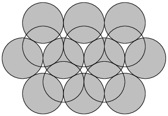
One can study the sphere packing problem in any dimension. In it is trivial, because the line can be completely covered with intervals. In , it is easy to guess that a hexagonal arrangement of circles is optimal, with each circle tangent to six others, but giving a rigorous proof of optimality is not completely straightforward and was first achieved in 1892 by Thue [50] (see [29] for a short, modern proof). In , the usual way oranges are stacked in grocery stores is optimal, but the proof is extraordinarily difficult. Hales completed a proof in 1998, with a lengthy combination of human reasoning and computer calculations [30]. One conceptual difficulty is that the solution is not at all unique in . In a technical sense, it is not unique in any dimension (even up to isometries), because density is a global property that is unchanged by, for example, removing a ball. However, in three dimensions there is a much deeper sort of non-uniqueness. One can form an optimal packing by stacking hexagonal layers, with each layer nestled into the gaps in the layer beneath it. As shown in Figure 1, the holes in a hexagonal lattice consist of two translates of the original lattice, and the next layer will sit above one of these two translates. For each layer, a binary choice must be made, and there are uncountably many ways to make these choices. (Each will be isometric to countably many others, but there remain uncountably many geometrically distinct packings, with many different symmetry groups.) All these packings are equally dense and perfectly natural. See [22] for a discussion of this issue in higherdimensions.
In four or more dimensions, no sharp density bounds are known. Instead, we merely have upper and lower bounds, which differ by a substantial factor. For example, in , the best upper bound known is more than times the density of the best packing known [16]. This factor grows exponentially with the dimension: the best lower bound known is a constant times in (see [7] and [52]), while the upper bound is (see [32]).
It may be surprising that these densities are so low. One way to think about it is in terms of volume growth in high dimensions. An -neighborhood of a ball in has volume times that of the ball, so when is large, there is far more volume near the surface of the ball than actually inside it. In low-dimensional sphere packings, most volume is contained within the balls, with a narrow fringe of gaps between them. In high-dimensional packings, the gaps occupy far more volume.
It is easy to prove a lower bound of for the sphere packing density in . In fact, this lower bound holds for every saturated packing (i.e., one in which there is no room for any additional spheres):
Lemma 2.1
Every saturated sphere packing in has density at least .
Proof.
Suppose the packing uses spheres of radius . No point in space can be distance or further from the nearest sphere center, since otherwise there would be room to center another sphere of radius at that point. This means we can cover space completely by doubling the radius of each sphere. Doubling the radius multiplies the volume by , and hence multiplies the density by at most (in fact, exactly if we count overlaps with multiplicity). Because the enlarged spheres cover all of space, the original spheres must cover at least a fraction. ∎
This argument sounds highly constructive (simply add more spheres to a packing until it becomes saturated), and indeed it is constructive in the logical sense. However, in practice it offers almost no insight into what dense packings look like, because it is difficult even to tell whether a high-dimensional packing is saturated.
In fact, it is completely unclear how to construct dense packings in high dimensions. One might expect the sphere packing problem to have a simple, uniform solution that would work in all dimensions. Instead, each dimension has its own charming idiosyncrasies, as we will see in Section 2.2. There is little hope of a systematic solution to the sphere packing problem in all dimensions. Even achieving density through a simple, explicit construction is an unsolved problem.
2.2 Lattices and periodic packings
The simplest sorts of packings are lattice packings. Recall that a lattice in is the integral span of a basis (i.e., it is a grid, possibly skewed). To form a sphere packing, one can center a sphere at each lattice point. The radius should be half the minimal distance between lattice points, so that the nearest spheres are tangent to each other.
There is no reason to expect that lattice packings should be the densest sphere packings, and they are probably not optimal in sufficiently high dimensions (for example, ten dimensions). However, lattices are very likely optimal in for and for some higher values of (including , , and ). See [24] for more details about lattices and packings in general.
For and , the lattice packing problem has been solved in . In fact, the densest lattices are unique in these dimensions (up to scaling and isometries), although that may not be true in every dimension, such as . For , the optimal lattices are all root lattices, the famous lattices that arise in Lie theory and are classified by Dynkin diagrams. Specifically, the densest lattices are (the integer lattice), (the hexagonal lattice), (the face-centered cubic lattice, which is also isomorphic to ), , , , , and . For , the Leech lattice is an optimal lattice packing; the proof will be discussed in Section 5.
The lattices are particularly simple, because they are formed by a checkerboard construction as a sublattice of index in :
To see why is not optimal in high dimensions, consider the holes in , i.e., the points in space that are local maxima for distance from the lattice. The integral points with odd coordinate sum are obvious candidates, and they are indeed holes, at distance from . However, there’s a slightly more subtle case, namely the point and its translates by . These points are at distance
from . When , this distance becomes , which is equal to the minimal distance between points in . That means these deep holes have become large enough that additional spheres can be placed in them. Doing so yields the root lattice, whose density is twice that of . (The and lattices are certain cross sections of .)
The and Leech lattices stand out among lattice packings, because all the spheres fit beautifully into place in a remarkably dense and symmetric way. There is no doubt that they are optimal packings in general, not just among lattices. Harmonic analysis ought to provide a proof, but as we will see in Section 5, a full proof has been elusive.
Periodic packings form a broader class of packings than lattice packings. A lattice can be viewed as the vertices of a tiling of space with parallelotopes (fundamental domains for the action by translation), but there’s no reason to center spheres only at the vertices. More generally, one can place them in the interior, or elsewhere on the boundary, and then repeat them periodically; such a packing is called a periodic packing. Equivalently, the sphere centers in a periodic packing form the union of finitely many translates of a lattice.
The packing, as defined above, is clearly periodic (the union of two translates of ). It is not quite as obvious that it is actually a lattice, but that is easy to check. The Leech lattice in can be defined by a similar, but more elaborate, construction involving filling in the holes in a lattice constructed using the binary Golay code (see [38] and Section 4.4 in Chapter 4 of [24]).
Philosophically, the construction of given above is somewhat odd, because itself is extraordinarily symmetrical, but the construction is not. Instead, it builds in two pieces. This situation is actually quite common when constructing a highly symmetric object. By neglecting part of the symmetry group, one can decompose the object into simpler pieces, which can each be understood separately. However, eventually one must exhibit the extra symmetry. The symmetry group of is generated by the reflections in the hyperplanes orthogonal to the minimal vectors of , and one can check that it acts transitively on those minimal vectors.
It is not known whether periodic packings achieve the maximal packing density in every dimension. However, they always come arbitrarily close: given any dense packing, one can take a large, cubical piece of it and repeat that piece periodically. To avoid overlaps, it may be necessary to remove some spheres near the boundary, but if the cube is large enough, then the resulting decrease in density will be small.
By contrast, it is not even known whether there exist saturated lattice packings in high dimensions. If not, then lattices cannot achieve more than half the maximal density, because one can double the density of a non-saturated lattice by filling in a hole together with all its translates by lattice vectors. It seems highly unlikely that there are saturated lattices in high dimensions, because a lattice is specified by a quadratic number of parameters, while there is an exponential volume of space in which holes could appear, so there are not enough degrees of freedom to control all the possible holes. However, this argument presumably cannot be made rigorous.
Despite all the reasons to think lattices are not the best sphere packings in high dimensions, the best asymptotic lower bounds known for sphere packing density use lattices. Ball’s bound in holds for lattice packings [7], and Vance’s bound, which improves it by an asymptotic factor of when is a multiple of four, uses not just lattices, but lattices that are modules over a maximal order in the quaternions [52]. Imposing algebraic structure may rule out the densest possible packings, but it makes up for that by offering powerful tools for analysis and proof.
2.3 Packing problems in other spaces
Packing problems are interesting in many metric spaces. The simplest situation is when the ambient space is compact, in which case the packing will involve only finitely many balls. The packing problem can then be formulated in terms of two different optimization problems for a finite subset of the metric space:
- 1.
What is the largest possible minimal distance between points?
- 2.
What is the largest possible size of a subset whose minimal distance is at least ?
The first fixes the number of balls and maximizes their size, while the second fixes the radius of the balls and maximizes the number. In Euclidean space, if we interpret the number of points as the number of points per unit volume, then both problems are the same by scaling invariance, but that does not hold in compact spaces. The two problems are equivalent, however, in the sense that a complete answer to one (for all values of or ) yields a complete answer to the other.
Packing problems arise naturally in many compact metric spaces, including spheres, projective spaces, Grassmannians [23, 4], and the Hamming cube (under Hamming distance, so packings are binary error-correcting codes). For a simplified example, suppose one wishes to treat a spherical tumor by beaming radiation at it. One would like to use multiple beams approaching it from different angles, so as to minimize radiation exposure outside of the tumor, and the problem of maximizing the angle between the beams is a packing problem in .
Packing problems are also important in non-compact spaces, but aside from Euclidean space we will not deal with them in this article, because defining density becomes much more subtle. See, for example, the foundational work by Bowen and Radin on defining packing density in hyperbolic space [11].
Packings on the surface of a sphere are known as spherical codes. Specifically, an optimal spherical code is an arrangement of points on a sphere that maximizes the minimal distance among configurations of its size. Spherical codes can be used as error-correcting codes (for example, in the toy model of radio transmission from Section 1.4, they are codes for a constant-power transmitter), and they also provide an elegant way to help characterize the many interesting spherical configurations that arise throughout mathematics.
One of the most attractive special cases of packing on a sphere is the kissing problem. How many non-overlapping unit balls can all be tangent to a central unit ball? The points of tangency on the central ball form a spherical code with minimal angle at least , and any such code yields a kissing configuration.
In , the kissing number is clearly six, but the answer is already not obvious in . The twelve vertices of an icosahedron work, but the tangent balls do not touch each other and can slide around. It turns out that there is no room for a thirteenth ball, but that was first proved only in 1953 by Schütte and van der Waerden [47].
In , Musin [42] showed that the kissing number is , but the answer is not known in (it appears to be ). In fact, the only higher dimensions for which the kissing problem has been solved are and , independently by Levenshtein [39] and by Odlyzko and Sloane [43]. The kissing numbers are in and in . Furthermore, these kissing configurations are unique up to isometries [9].
The kissing number of is achieved by the root lattice through its minimal vectors. Specifically, there are permutations of and vectors of the form with an even number of minus signs. Thus, is not only the densest lattice packing in , but it also has the highest possible kissing number. Similarly, the Leech lattice in achieves the kissing number of .
In general, however, there is no reason to believe that the densest packings will also have the highest kissing numbers. The packing density is a global property, while the kissing number is purely local and might be maximized in a way that cannot be extended to a dense packing. That appears to happen in many dimensions [24]. Instead of being typical, compatibility between the optimal local and global structures is a remarkable occurrence.
3 The Thomson Problem and Universal Optimality
3.1 Physics on surfaces
The Thomson problem [49, p. 255] asks for the minimal-energy configuration of classical electrons confined to the unit sphere . In other words, the particles interact via the Coulomb potential at Euclidean distance . This model was originally intended to describe atoms, before quantum mechanics or even the discovery of the nucleus. Thomson hoped it would explain the periodic table. Of course, subsequent discoveries have shown that it is a woefully inadequate atomic model, but it remains of substantial scientific interest, and its variants describe many real-worldsystems.
For example, imagine mixing together two immiscible liquids, such as oil and water. The oil will break up into tiny droplets, evenly dispersed within the water, but they will rapidly coalesce and the oil will separate from the water. Cooks have long known that one can prevent this separation by using emulsifiers. One type of emulsion is a Pickering emulsion, in which tiny particles collect on the boundaries of oil droplets, which prevents coalescence (the particles bounce off each other).
More generally, colloidal particles often adsorb to the interface between two different liquids. See, for example, Figure 2, which shows charged particles made of polymethyl methacrylate (i.e., plexiglas) in a mixture of water and cyclohexyl bromide. Notice that the particles on the surface of the droplet have spread out into a fairly regular arrangement due to their mutual repulsion, and they are repelling the remaining particles away from the surface.

These particles are microscopic, yet large enough that they can accurately be described using classical physics. Thus, the generalized Thomson problem is an appropriate model. See [12] for more details on these sorts of materials.
Consider the case of particles on the unit sphere in . Given a finite subset and a potential function , define the potential energy by
For each positive integer and each , we seek an -element subset that minimizes compared to all other choices of with . The use of squared distance instead of distance is not standard in physics, but it will prove mathematically convenient. The function is defined only on because no squared distance larger than can occur on the unit sphere.
Typically will be decreasing (so the force is repulsive) and convex. In fact, the most natural potential functions to use are the completely monotonic functions, i.e., smooth functions satisfying for all integers . For example, inverse power laws (with ) are completely monotonic.
3.2 Varying the potential function
As we vary the potential function above, how do the optimal configurations change? From the physics perspective, this question appears silly, because the potential is typically determined by fundamental physics. However, from a mathematical perspective it is a critical question, because it places the individual optimization problems into a richer context.
As we vary the potential function, the optimal configurations will vary in some family. This family may not be connected, because the optimum may abruptly jump as the potential function passes some threshold, and different components may have different dimensions [15]. Nevertheless, we can use the local dimension of the family as a crude measure of the complexity of an optimum: we compute the dimension of the space of perturbed configurations that minimize energy for perturbations of the potential function. Call this dimension the parameter count of the configuration.

Figure 3 (taken from [8]) shows the parameter counts for the configurations minimizing Coulomb energy on with through points. The figure is doubly conjectural: in almost all of these cases, no proof is known that the supposed optima are truly optimal or that the parameter counts are correct. However, the experimental evidence leaves little doubt.
3.3 Universal optimality
When one varies the potential function, the simplest case is when the optimal configuration never varies. Call a configuration universally optimal if it minimizes energy for all completely monotonic potential functions.
A universal optimum is automatically an optimal spherical code: for the potential function with large, the energy is asymptotically determined by the minimal distance, and minimizing energy requires maximizing the minimal distance. However, optimal spherical codes are rarely universally optimal. For every number of points in every dimension, there exists some optimal code, but universal optima appear to be far less common.
In , there is an -point universal optimum for each , namely the vertices of a regular -gon. In , the situation is more complicated. Aside from degenerate cases with three or fewer points, there are only three universal optima, namely the vertices of a regular tetrahedron, octahedron, or icosahedron [17]. The cube and dodecahedron are not even optimal, let alone universally optimal, since one can lower energy by rotating a facet.
The first case for which there is no universal optimum is five points in . There are two natural configurations: a triangular bipyramid, with an equilateral triangle on the equator together with the north and south poles, and a square pyramid, with its top at the north pole and its base slightly below the equator. This second family depends on one parameter, the height of the pyramid. The triangular bipyramid is known to minimize energy for several inverse power laws [48], but it is not even a local minimum when they are sufficiently steep, in which case square pyramids seem to become optimal.
Conjecture 3.1
For every completely monotonic potential function, either the triangular bipyramid or a square pyramid minimizes energy among five-point configurations in .
| Description | ||
|---|---|---|
| regular simplex | ||
| regular cross polytope | ||
| regular -gon | ||
| regular icosahedron | ||
| regular -cell | ||
| hemicube | ||
| Schläfli graph | ||
| equiangular lines | ||
| root system | ||
| isotropic subspaces | ||
| strongly regular graph | ||
| Higman-Sims graph | ||
| McLaughlin graph | ||
| isotropic subspaces | ||
| equiangular lines | ||
| iterated kissing configuration | ||
| Leech lattice minimal vectors | ||
| isotropic subspaces ( is a prime power) |
For , the universal optima in have not been completely classified. Table 1 shows a list of the known cases (proved in [17]). Each of them is a fascinating mathematical object. For example, the points in correspond to the lines on a cubic surface.
The first five lines in the table list the regular polytopes with simplicial facets. The next four lines list the root system and certain semiregular polytopes obtained as cross sections. The next eight lines list the minimal vectors of the Leech lattice and certain cross sections. If this were the complete list, it would feel reasonable, but the last line is perplexing. It describes another infinite sequence of universal optima, constructed from geometries over in [13] and recognized as optimal codes in [40]. How many more such cases remain to be constructed?
Another puzzling aspect of Table 1 is the gap between and dimensions. Are there really no universal optima in these dimensions, aside from the simplices and cross polytopes? Or do we simply lack the imagination needed to discover them? Extensive computer searches [8] suggest that the table is closer to complete than one might expect, but probably not complete. Specifically, there are a -point configuration in and a -point configuration in that appear to be universally optimal, but these are the only conjectural cases that have been located.
Almost all of the results tabulated in Table 1 can be deduced from the following theorem. It generalizes a theorem of Levenshtein [40], which says that these configurations are all optimal codes. The one known case not covered by the theorem is the regular -cell, which requires a different argument [17].
To state the theorem, we will need two definitions. A spherical -design in is a finite subset of the sphere such that for every polynomial of total degree at most , the average of over equals its average over the entire sphere. Spherical -designs can be thought of as sets giving quadrature rules (i.e., numerical integration schemes) that are exact for polynomials of degree up to . An -distance set is a set for which distances occur between distinct points.
Theorem 3.2 (Cohn and Kumar [17])
Every -distance set that is a spherical -design is universally optimal.
The proof of this theorem uses linear programming bounds, which are developed in the next section.
4 Proof Techniques: Linear Programming Bounds
4.1 Constraints on the pair correlation function
In this section, we will discuss techniques for proving lower bounds on potential energy. In particular, we will develop linear programming bounds and briefly explain how they are used to prove Theorem 3.2.
They are called “linear programming bounds” because linear programming can be used to optimize them, but no knowledge of linear programming is required to understand how the bounds work. They were originally developed by Delsarte for discrete problems in coding theory [25], extended to continuous packing problems in [26, 32], and adapted for potential energy minimization by Yudin and his collaborators [55, 35, 36, 1, 2]. In this section, we will focus on spherical configurations, although the techniques work in much greater generality.
Given a finite subset of , define its distance distribution by
where denotes the inner product in . In physics terms, is the pair correlation function; it measures how often each pairwise distance occurs (the inner product is a natural way to gauge distance on the sphere). Linear programming bounds are based on proving certain linear inequalities involving the numbers . These inequalities are crucial because the potential energy can be expressed in terms of the distance distribution by
| (4.1) |
since . (Although (4.1) sums over uncountably many values of , only finitely many of the summands are nonzero.) Energy is a linear function of , and the linear programming bound is the minimum of this function subject to the linear constraints on , which makes it the solution to a linear programming problem in infinitely many variables.
To begin, there are several obvious constraints on the distance distribution. Let . Then for all , for , , and
The power of linear programming bounds comes from less obvious constraints. For example, To see why, notice that
More generally, there is an infinite sequence of polynomials (independent of , but depending on the dimension ) , with , such that for each ,
| (4.2) |
(In fact, we can take , , and .) This inequality is nontrivial, because these polynomials are frequently negative. For example, looks like this:
![[Uncaptioned image]](1003.3053v2/gegen.png)
The polynomials are called ultraspherical polynomials, and they are characterized by orthogonality on the interval with respect to the measure . In other words, for ,
This relationship determines the polynomials up to scaling, as the Gram-Schmidt orthogonalization of the monomials with respect to this inner product. The sign of the scaling constant is determined by , and the magnitude of the constant is irrelevant for (4.2).
In fact, these polynomials have a far stronger property than just (4.2): they are positive-definite kernels. That is, for any and any points , the matrix is positive semidefinite. This implies (4.2) because the sum of the entries of a positive-semidefinite matrix is nonnegative. Schoenberg [45] proved that every continuous positive-definite kernel on must be a nonnegative linear combination of ultraspherical polynomials.
4.2 Zonal spherical harmonics
As an illustration of the role of representation theory, in this section we will derive the ultraspherical polynomials as zonal spherical harmonics and verify that they satisfy (4.2). The reader who is willing to take that on faith can skip the derivation.
The orthogonal group acts on by isometries, and hence is a unitary representation of . To begin, we will decompose this representation into irreducibles. Let be the subspace of functions on defined by polynomials on of total degree at most . We have , and each is a finite-dimensional representation of , with dense in . To convert this filtration into a direct sum decomposition, let and define to be the orthogonal complement of within (with respect to the usual inner product on ). Then is still preserved by , and the entire space breaks up as
(The hat indicates the completion of the algebraic direct sum.) The functions in are known as spherical harmonics of degree , because is an eigenspace of the spherical Laplacian, but we will not need that characterization of them.
For each , evaluating at defines a linear map on . Thus, there exists a unique vector such that for all ,
where denotes the inner product on from . The map is called a reproducing kernel.
For each and ,
Thus, , by the uniqueness of . It follows that is invariant under the stabilizer of in . In other words, it is invariant under rotations about the axis through , so it is effectively a function of only one variable, the inner product with . Such a function is called a zonal spherical harmonic.
We can define by
These polynomials certainly satisfy (4.2), because
and in fact they are positive-definite kernels because is the Gram matrix of the vectors .
The functions are in orthogonal subspaces, and hence the polynomials must be orthogonal with respect to the measure on obtained by projecting the surface measure of onto the axis from to . The following simple calculation shows that the measure is proportional to . Consider the spherical shell defined by
If we set , then the remaining coordinates satisfy
and the volume is proportional to . If we divide by to normalize, then as we find that the density of the surface measure with is proportional to , as desired.
The degree of is at most , and because is orthogonal to , the degree can be less than only if is identically zero. That cannot be the case (for ), since otherwise evaluating at would be identically zero. If it were, then it would follow from that evaluating at each point is identically zero, and thus that is trivial. However, , and hence is nontrivial.
Thus, the polynomials defined above have degree , satisfy (4.2), and have the desired orthogonality relationship.
4.3 Linear programming bounds
Let be a finite subset and let be its distance distribution. To make use of the linear constraints on discussed in Section 4.1, we will use the dual linear program. In other words, we will take linear combinations of the constraints so as to obtain a lower bound on energy.
We introduce new real variables and specifying which linear combination to take. Suppose we add times , times
(with for ), and times the constraint (with for ). We find that
using the normalization . Define . Then
because . If we choose and so that for , then the energy will be bounded below by , by (4.1).
The equation just means that (because we have assumed only that ). Thus, we have proved the following bound:
Theorem 4.1 (Yudin [55])
Suppose satisfies for and for . Then for every finite subset ,
To prove Theorem 3.2, one can optimize the choice of the auxiliary function in Theorem 4.1. Suppose is an -distance set and a spherical -design, and is completely monotonic. In the proof of Theorem 4.1, equality holds if and only if for every inner product that occurs between points in and whenever and . The latter equation automatically holds for because is a -design. Let be the unique polynomial of degree at most that agrees with to order at each of the inner products between distinct points in , so that satisfies the other condition for equality. The inequality follows easily from a remainder theorem for Hermite interpolation (using the complete monotonicity of ). The most technical part of the proof is the verification that the coefficients of are nonnegative. For any single configuration, it can be checked directly; for the general case, see [17].
4.4 Semidefinite programming bounds
Semidefinite programming bounds, introduced by Schrijver [46] and generalized by Bachoc and Vallentin [5], extend the idea of linear programming bounds by looking at triple (or even higher) correlation functions, rather than just pair correlations. Linear constraints are naturally replaced with semidefinite constraints, and the resulting bounds can be optimized by semidefinite programming.
This method is a far-reaching generalization of linear programming bounds, and it has led to several sharp bounds that could not be obtained previously [6, 21]. However, the improvement in the bounds when going from pairs to triples is often small, while the computational price is high. One of the most interesting conceptual questions in this area is the trade-off between higher correlations and improved bounds. When studying -point configurations in using -point correlation bounds, how large does need to be to prove a sharp bound? Clearly would suffice, and for the cases covered by Theorem 3.2 it is enough to take . Aside from a handful of cases in which works, almost nothing is known in between. (Cases with seem too difficult to handle computationally.) This question is connected more generally to the strength of LP and SDP hierarchies for relaxations of NP-hard combinatorial optimization problems [37].
It is also related to a conjecture of Torquato and Stillinger [51], who propose that for packings that are disordered (in a certain technical sense), in sufficiently high dimensions the two-point constraints are not only necessary but also sufficient for the existence of a packing with a given pair correlation function. They show that this conjecture would lead to packings of density in , by exhibiting the corresponding pair correlation functions. The problem of finding a hypothetical pair correlation function that maximizes the packing density, subject to the two-point constraints, is dual to the problem of optimizing the linear programming bounds.
5 Euclidean Space
5.1 Linear programming bounds in Euclidean space
Linear programming bounds can also be applied to packing and energy minimization problems in Euclidean space, with Fourier analysis taking the role played by the ultraspherical polynomials in the spherical case. In this section, we will focus primarily on packing, before commenting on energy minimization at the end. The theory is formally analogous to that in compact spaces, but the resulting optimization problems are quite a bit deeper and more subtle, and the most exciting applications of the theory remain conjectures.
We will normalize the Fourier transform of an function by
(In this section, will not denote a potential function.) The fundamental technical tool is the Poisson summation formula for a lattice , which holds for all Schwartz functions (i.e., smooth functions all of whose derivatives are rapidly decreasing):
Here, is the volume of a fundamental parallelotope, and is the dual lattice defined by
Given any basis of , the dual basis with respect to is a basis of .
Theorem 5.1 (Cohn and Elkies [16])
Let be a Schwartz function such that . If for and for all , then the sphere packing density in is at most
Of course, means when is odd. The restriction to Schwartz functions can be replaced with milder assumptions [16, 17].
The hypotheses and conclusion of Theorem 5.1 are invariant under rotation about the origin, so without loss of generality we can symmetrize and assume it is a radial function. Thus, optimizing the bound in Theorem 5.1 amounts to optimizing the choice of a function of one (radial) variable.
It is not hard to prove Theorem 5.1 for the special case of lattice packings. Suppose is a lattice, and rescale so we can assume the minimal vector length is (i.e., the packing uses balls of radius ). The density is the volume of a sphere of radius , which is , times the number of spheres occurring per unit volume in space. The latter factor is , because there is one sphere for each fundamental cell of the lattice, and hence the density equals
Now we apply Poisson summation to see that
The left side is bounded above by , because all the other terms come from and are thus nonpositive by assumption. The right side is bounded below by , because all the other terms are nonnegative. Thus,
which is equivalent to the density bound in Theorem 5.1.
The proof in the general case is completely analogous. It suffices to prove the bound for all periodic packings (because they come arbitrarily close to the maximal density), and one can apply a version of Poisson summation for summing over translates of a lattice. See [16] for the details, as well as for an explanation of the analogy between these linear programming bounds and those for compact spaces.
5.2 Apparent optimality of and the Leech lattice
Theorem 5.1 does not explain how to choose the function , and for the optimal choice of is unknown. However, one can use numerical methods to optimize the density bound, for example by choosing to be times a polynomial in (so that the Fourier transform can be easily computed) and then optimizing the choice of the polynomial. For , the results were collected in Table 3 of [16], and in each case the bound is the best one known, but they are typically nowhere near sharp. For example, when , the upper bound is roughly times the best packing density known. That was an improvement on the previous bound, which was off by a factor of , but the gap remains enormous.
However, for , , or , Theorem 5.1 appears to be sharp:
Conjecture 5.2 (Cohn and Elkies [16])
For , , or , there exists a function that proves a sharp bound in Theorem 5.1 (for the hexagonal, , or Leech lattice, respectively).
The strongest numerical evidence comes from [18]: for the bound is sharp to within a factor of . Similar accuracy can be obtained for or , although only was reported in [18]. Of course, for the sphere packing problem has already been solved, but Conjecture 5.2 is open.
This apparent sharpness is analogous to the sharpness of the linear programming bounds for the kissing number in , , and . In that problem, it would have sufficed to prove any bound less than the answer plus one, because the kissing number must be an integer, but the bounds in fact turn out to be exact integers. In the case of the sphere packing problem, the analogous exactness is needed (because packing density is not quantized), and fortunately it appears to be true.
Examining the proof of Theorem 5.1 gives simple conditions for when the bound can be sharp for a lattice , analogous to the conditions for Theorem 4.1: must vanish at each nonzero point in and must vanish at each nonzero point in . In fact, the same must be true for all rotations of , so and must vanish at these radii (even if they are not radial functions). Unfortunately, it seems difficult to control the behavior of and simultaneously.
For the special case of lattices, however, it is possible to complete a proof.
Theorem 5.3 (Cohn and Kumar [18])
The Leech lattice is the unique densest lattice in , up to scaling and isometries.
The proof uses Theorem 5.1 to show that no sphere packing in can be more than slightly denser than the Leech lattice, and that every lattice as dense as the Leech lattice must be very close to it. However, the Leech lattice is a locally optimal packing among lattices, and the bounds can be made close enough to complete the proof. This approach also yields a new proof of optimality and uniqueness for (previously shown in [10] and [53]).
One noteworthy hint regarding the optimal functions in and is an observation of Cohn and Miller [20] about the Taylor series coefficients of . It is more convenient to use the rescaled function , where when and when . Then , and without loss of generality let this value be . Assuming is radial, we can view and as functions of one variable and ask for their Taylor series coefficients. Only even exponents occur by radial symmetry, so the first nontrivial terms are quadratic. Cohn and Miller noticed that the quadratic coefficients appear to be rational numbers, as shown in Table 2. The quartic terms seem more subtle, and it is not clear whether they are rational as well. If they are, then their denominators are probably much larger.
| function | order | coefficient | conjecture | |
|---|---|---|---|---|
| ? | ||||
| ? | ||||
| ? | ||||
| ? |
More generally, one can study not just the sphere packing problem, but also potential energy minimization in Euclidean space. The total energy of a periodic configuration will be infinite, because each distance occurs infinitely many times, but one can instead try to minimize the average energy per particle. Some of the densest packings minimize more general forms of energy, but others do not, and simulations lead to many intriguing structures [19].
Cohn and Kumar [17] proved linear programming bounds for energy and made a conjecture analogous to Conjecture 5.2:
Conjecture 5.4 (Cohn and Kumar [17])
For , , or , the linear programming bounds for potential energy minimization in are sharp for every completely monotonic potential function (for the hexagonal, , or Leech lattice, respectively).
This universal optimality would be a dramatic strengthening of mere optimality as packings. It is not even known in the two-dimensional case.
6 Future Prospects
The most pressing question raised by this work is how to prove that the hexagonal lattice, , and the Leech lattice are universally optimal in Euclidean space. Linear programming bounds reduce this problem to finding certain auxiliary functions of one variable, and the optimal functions can even be computed to high precision, but so far there is no proof that they truly exist.
More generally, can we classify the universal optima in a given space? No proof is known even that the list of examples in is complete, although it very likely is. Each of the known universal optima is such a remarkable mathematical object that a classification would be highly desirable: if there are any others out there, we ought to find them.
One noteworthy case is equiangular line configurations in complex space. Do there exist unit vectors such that for , is independent of and (in which case one can show it must be )? In other words, the complex lines through these vectors are equidistant under the Fubini-Study metric in . Zauner [56] conjectured that the answer is yes for all , and substantial numerical evidence supports that conjecture [44], but only finitely many cases have been proved. A collection of vectors with this property gives an -point universal optimum in , by Theorem 8.2 in [17]. This case is particularly unusual, because normally the difficulty is in proving optimality for a configuration that has already been constructed, rather than constructing one that has already been proved optimal (should it exist).
These equiangular line configurations are in fact closely analogous to Hadamard matrices. They can be characterized as exactly the simplices in that are projective -designs (where a simplex is simply a set of points for which all pairwise distances are equal). Similarly, Hadamard designs, which are an equivalent variant of Hadamard matrices [3], are symmetric block -designs that are simplices under the Hamming distance between blocks. The existence of Hadamard matrices of all orders divisible by four is a famous unsolved problem in combinatorics, and perhaps the problem of equiangular lines in will be equally difficult.
These two problems are finely balanced between order and disorder. Any Hadamard matrix or equiangular line configuration must have considerable structure, but in practice they frequently seem to have just enough structure to be tantalizing, without enough to guarantee a clear construction. This contrasts with many of the most symmetrical mathematical objects, which are characterized by their symmetry groups: once you know the full group and the stabilizer of a point, it is often not hard to deduce the structure of the complete object. That seems not to be possible in either of these two problems, and it stands as a challenge to find techniques that can circumvent this difficulty.
In conclusion, packing and energy minimization problems exhibit greatly varying degrees of symmetry and order in their solutions. In certain cases, the solutions are extraordinary mathematical objects such as or the Leech lattice. Sometimes this can be proved, and sometimes it comes down to simply stated yet elusive conjectures. In other cases, the solutions may contain defects or involve unexpectedly complicated structures. Numerical experiments suggest that this is the default behavior, but it is difficult to predict exactly when or how it will occur. Finally, in rare cases there appears to be order of an unusually subtle type, as in the complex equiangular line problem, and this type of order remains a mystery.
Acknowledgments
I am grateful to James Bernhard, Tom Brennan, Tzu-Yi Chen, Donald Cohn, Noam Elkies, Abhinav Kumar, Achill Schürmann, Sal Torquato, Frank Vallentin, Stephanie Vance, Jeechul Woo, and especially Nadia Heninger for their valuable feedback on this paper.
References
- [1] N. N. Andreev, An extremal property of the icosahedron, East J. Approx. 2 (1996), 459–462.
- [2] N. N. Andreev, Location of points on a sphere with minimal energy, Proc. Steklov Inst. Math. 219 (1997), 20–24.
- [3] E. F. Assmus, Jr. and J. D. Key, Designs and Their Codes, Cambridge Tracts in Mathematics 103, Cambridge University Press, Cambridge, 1992.
- [4] C. Bachoc, Linear programming bounds for codes in Grassmannian spaces, IEEE Trans. Inform. Theory 52 (2006), 2111–2125.
- [5] C. Bachoc and F. Vallentin, New upper bounds for kissing numbers from semidefinite programming, J. Amer. Math. Soc. 21 (2008), 909–924.
- [6] C. Bachoc and F. Vallentin, Optimality and uniqueness of the spherical code, J. Combin. Theory Ser. A 116 (2009), 195–204.
- [7] K. Ball, A lower bound for the optimal density of lattice packings, Internat. Math. Res. Notices 1992, 217–221.
- [8] B. Ballinger, G. Blekherman, H. Cohn, N. Giansiracusa, E. Kelly, and A. Schürmann, Experimental study of energy-minimizing point configurations on spheres, Experiment. Math. 18 (2009), 257–283.
- [9] E. Bannai and N. J. A. Sloane, Uniqueness of certain spherical codes, Canad. J. Math. 33 (1981), 437–449.
- [10] H. F. Blichfeldt, The minimum values of positive quadratic forms in six, seven and eight variables, Math. Z. 39 (1935), 1–15.
- [11] L. Bowen and C. Radin, Densest packing of equal spheres in hyperbolic space, Discrete Comput. Geom. 29 (2003), 23–39.
- [12] M. Bowick and L. Giomi, Two-dimensional matter: order, curvature and defects, Advances in Physics 58 (2009), 449–563.
- [13] P. J. Cameron, J. M. Goethals, and J. J. Seidel, Strongly regular graphs having strongly regular subconstituents, J. Algebra 55 (1978), 257–280.
- [14] H. Cohn, New upper bounds on sphere packings II, Geom. Topol. 6 (2002), 329–353.
- [15] H. Cohn, J. H. Conway, N. D. Elkies, and A. Kumar, The root system is not universally optimal, Experiment. Math. 16 (2007), 313–320.
- [16] H. Cohn and N. D. Elkies, New upper bounds on sphere packings I, Ann. of Math. 157 (2003), 689–714.
- [17] H. Cohn and A. Kumar, Universally optimal distribution of points on spheres, J. Amer. Math. Soc. 20 (2007), 99–148.
- [18] H. Cohn and A. Kumar, Optimality and uniqueness of the Leech lattice among lattices, Ann. of Math. 170 (2009), 1003–1050.
- [19] H. Cohn, A. Kumar, and A. Schürmann, Ground states and formal duality relations in the Gaussian core model, Phys. Rev. E 80 (2009), 061116:1–7.
- [20] H. Cohn and S. D. Miller, Some conjectures on optimal auxiliary functions for sphere packing, preprint, 2010.
- [21] H. Cohn and J. Woo, Three-point bounds for energy minimization, preprint, 2010.
- [22] J. H. Conway and N. J. A. Sloane, What are all the best sphere packings in low dimensions?, Discrete Comput. Geom. 13 (1995), 383–403.
- [23] J. H. Conway, R. H. Hardin, and N. J. A. Sloane, Packing lines, planes, etc.: packings in Grassmannian spaces, Experiment. Math. 5 (1996), 139–159.
- [24] J. H. Conway and N. J. A. Sloane, Sphere Packings, Lattices and Groups, third edition, Grundlehren der Mathematischen Wissenschaften 290, Springer, New York, 1999.
- [25] P. Delsarte, Bounds for unrestricted codes, by linear programming, Philips Res. Rep. 27 (1972), 272–289.
- [26] P. Delsarte, J. M. Goethals, and J. J. Seidel, Spherical codes and designs, Geom. Dedicata 6 (1977), 363–388.
- [27] F. J. Dyson, A Brownian-motion model for the eigenvalues of a random matrix, J. Math. Phys. 3 (1962), 1191–1198.
- [28] L. Fejes Tóth, Regular Figures, Pergamon Press, Macmillan, New York, 1964.
- [29] T. C. Hales, Cannonballs and honeycombs, Notices Amer. Math. Soc. 47 (2000), 440–449.
- [30] T. C. Hales, A proof of the Kepler conjecture, Ann. of Math. 162 (2005), 1065–1185.
- [31] M. Hazewinkel, W. Hesselink, D. Siersma, and F. D. Veldkamp, The ubiquity of Coxeter-Dynkin diagrams (an introduction to the –– problem), Nieuw Arch. Wisk. 25 (1977), 257–307.
- [32] G. A. Kabatiansky and V. I. Levenshtein, Bounds for packings on a sphere and in space, Probl. Inf. Transm. 14 (1978), 1–17.
- [33] A. I. Khinchin, Mathematical Foundations of Information Theory, Dover Publications, Inc., New York, 1957.
- [34] F. Klein, Lectures on the Icosahedron and the Solution of Equations of the Fifth Degree, second edition, Dover Publications, Inc., New York, 1956.
- [35] A. V. Kolushov and V. A. Yudin, On the Korkin-Zolotarev construction, Discrete Math. Appl. 4 (1994), 143–146.
- [36] A. V. Kolushov and V. A. Yudin, Extremal dispositions of points on the sphere, Anal. Math. 23 (1997), 25–34.
- [37] M. Laurent, A comparison of the Sherali-Adams, Lovász-Schrijver, and Lasserre relaxations for – programming, Math. Oper. Res. 28 (2003), 470–496.
- [38] J. Leech, Notes on sphere packings, Canad. J. Math. 19 (1967), 251–267.
- [39] V. I. Levenshtein, On bounds for packings in -dimensional Euclidean space, Soviet Math. Dokl. 20 (1979), 417–421.
- [40] V. I. Levenshtein, Designs as maximum codes in polynomial metric spaces, Acta Appl. Math. 29 (1992), 1–82.
- [41] H. Löwen, Fun with hard spheres, in Statistical Physics and Spatial Statistics (Wuppertal, 1999), 295–331, Lecture Notes in Phys. 554, Springer, New York, 2000.
- [42] O. Musin, The kissing number in four dimensions, Ann. of Math. 168 (2008), 1–32.
- [43] A. M. Odlyzko and N. J. A. Sloane, New bounds on the number of unit spheres that can touch a unit sphere in dimensions, J. Combin. Theory Ser. A 26 (1979), 210–214.
- [44] J. M. Renes, R. Blume-Kohout, A. J. Scott, and C. M. Caves, Symmetric informationally complete quantum measurements, J. Math. Phys. 45 (2004), 2171–2180.
- [45] I. J. Schoenberg, Positive definite functions on spheres, Duke Math. J. 9 (1942), 96–107.
- [46] A. Schrijver, New code upper bounds from the Terwilliger algebra and semidefinite programming, IEEE Trans. Inform. Theory 51 (2005), 2859–2866.
- [47] K. Schütte and B. L. van der Waerden, Das Problem der dreizehn Kugeln, Math. Ann. 125 (1953), 325–334.
- [48] R. E. Schwartz, The electron case of Thomson’s problem, preprint, 2010, arXiv:1001.3702.
- [49] J. J. Thomson, On the structure of the atom, Phil. Mag. 7 (1904), 237–265.
- [50] A. Thue, Om nogle geometrisk-taltheoretiske Theoremer, Forhandlingerne ved de Skandinaviske Naturforskeres 14 (1892), 352–353.
- [51] S. Torquato and F. Stillinger, New conjectural lower bounds on the optimal density of sphere packings, Experiment. Math. 15 (2006), 307–331.
- [52] S. Vance, Lattices and sphere packings in Euclidean space, Ph.D. dissertation, University of Washington, 2009.
- [53] N. M. Vetčinkin, Uniqueness of classes of positive quadratic forms on which values of the Hermite constant are attained for , Proc. Steklov Inst. Math. 152 (1982), 37–95.
- [54] D. Weaire and R. Phelan, A counterexample to Kelvin’s conjecture on minimal surfaces, Phil. Mag. Lett. 69 (1994), 107–110.
- [55] V. A. Yudin, Minimum potential energy of a point system of charges, Discrete Math. Appl. 3 (1993), 75–81.
- [56] G. Zauner, Quantendesigns: Grundzüge einer nichtkommutativen Designtheorie, Ph.D. dissertation, Universität Wien, 1999.