Emergence of rigidity at the structural glass transition: a first principle computation

The shear-modulus is an unambiguous measure of the mechanical stability of materials. When one cools a glass-former below its glass transition, there appears a non-zero shear modulus on laboratory-accessible time scales. The understanding of the mechanism through which this rigidity emerges at the glass transition is a basic problem in condensed matter physics.

A standard view on glasses is to regard them as very slow liquids with extremely high shear-viscosity [1]. Visco-elastic measurements show that super-cooled liquids and various soft-glassy materials behave as solids: The elastic modulus develops at low frequencies a plateau, which extends to lower and lower frequencies by lowering temperature or increasing density (see [2, 3] and references therein). Thus glasses aquire rigidity progressively. This feature is remarkably different from ordinary transitions from liquid to crystal where the rigidity appears abruptly at the 1st order phase transition.

Among various theoretical attempts, the so-called random first order theory (RFOT)[4] provides a useful working ground to study the super-cooled liquids and glasses in a unified manner [5]. At the mean field level it is backed up by some microscopic approaches. On the one hand, it is intimately related to the mode-coupling theory (MCT) concerning the dynamics at relatively high temperatures [6]. On the other hand, the so-called cloned liquid approach which combines the traditional liquid theory and the replica method allows one to compute thermodynamic static quantities at lower temperatures[7, 8, 9]. This approach is currently the main first-principle approach to studying properties of the glass phase. It has been so far limited to computing thermodynamic properties, in particular the ‘complexity’ giving the entropy associated with the number of glass states. One of the major present challenges is to understand how the nucleation processes allowing to jump between glass states, which are not taken into account in the simplest RFOT scenario, can be included into this scheme. These processes are in particular crucial to explain why the mean field prediction of a dynamical transition at the dynamical (MCT) temperature $T_{c}$ breaks down, and is replaced by a rapid increase of the relaxation time when the temperature gets close to $T_{c}$. Attempts in this direction include the mosaic theory of [5] and the study of long-range interactions [10].

We shall extend the cloned liquid approach in order to compute the static shear-response of glasses. We identify the plateau modulus mentioned above by distinguishing intra-state and inter-state stress fluctuations. When applied to mesoscopic samples, this approach predicts that the stress vs strain curve should have an intermittent behaviour.

Models - We consider a system of $N$ particles ($i=1,2,\ldots,N$) at position ${\bf r}_{i}=(x_{i},y_{i},z_{i})$ in the laboratory frame, which are interacting with each other via two body potentials, $H(\{{\bf r}_{ij}\})=\sum_{i<j}v_{ij}(r_{ij})\ ,$ where ${\bf r}_{ij}={\bf r}_{i}-{\bf r}_{j}$ and $r_{ij}=|{\bf r}_{ij}|$. In order to study the rigidity against simple shear deformation, we consider a system of particles in a container with two boundary walls which are normal to the $z$-axis and separated from each other by distance $L_{z}$ as shown in Fig.1. To impose a shear strain $\gamma$ on the system, we simply displace the top wall by an amount $\gamma L_{z}$ into $x$-direction. Then it is convenient to introduce a sheared frame with $x^{\prime}$,$y^{\prime}$ and $z^{\prime}$ which are related to the laboratory frame as, $(x,y,z)=(x^{\prime}+z^{\prime}\gamma,y^{\prime},z^{\prime})$. The volume of the system $V$ and the number density $\rho=N/V$ remain constant under this shear.

Shear-modulus - The total free-energy $F(\gamma)$ of the system can be written as

with $\beta^{-1}=k_{\rm B}T$ being the inverse temperature. The ideal gas part of the free-energy is omitted because it does not change. Note that the integration over the interior volume of the container is taken using the sheared frame ${\bf r}^{\prime}=(x^{\prime},y^{\prime},z^{\prime})$ for which the integration range ${\cal V}$ is independent of the shear $\gamma$.

Taking infinitesimal shear, the free-energy can be expanded formally as $F(\gamma)=F(0)+N\langle\sigma\rangle\gamma+\frac{N}{2}\mu\gamma^{2}+O(\gamma^{3})$, where the shear-stress $\sigma$ and the shear-modulus $\mu$ are:

with

where $\langle\ldots\rangle$ denotes a thermal average evaluated with zero strain $\gamma=0$. We have introduced short hand notations like $\hat{x}_{ij}=(x_{i}-x_{j})/r_{ij}$, and the prime stands for differentiation. The 1st term $\langle b\rangle$ in the definition of $\mu$ in Eq. (2) is called the Born term. It represents the instantaneous response of the system against shear $G(\tau=0)$ (see below), which is finite even in liquids. The 2nd term is the correction term due to thermal fluctuations of the shear-stress.

This type of fluctuation formula for the static elastic constants is well known [13, 25]. In liquids, it is equivalent to the static limit of the Green-Kubo formula which relates the dynamic linear response against shear $\delta\sigma(t)=\int_{-\infty}^{t}dt^{\prime}G(t-t^{\prime})\dot{\gamma}(t^{\prime})$ to the shear-stress autocorrelation function $\langle\sigma(t)\sigma(t^{\prime})\rangle$ by $G(\tau)=\beta\langle\sigma(\tau)\sigma(0)\rangle$. Linear visco-elastic measurements give access to the complex dynamical modulus $G(\omega)=\omega G^{*}(\omega)$.

Boundary condition to shear - Let us pause here to discuss more explicitely the boundary condition. First of all, it is obvious that the boundary walls should not be strictly translationally invariant to exert shear on the system. On the other hand, we wish the system to maintain translational invariance at least on macroscopic scales. We thus assume that the walls are built from a quenched random configuration of particles, as shown in Fig. 1 so that the system keeps translational invariance in a statistical sense.

Because of the translational invariance at macroscopic scales, the thermodynamic free-energy density $\lim_{V\to\infty}F(\gamma)/V$ is independent of $\gamma$. This also happens in crystals, as discussed recently [11]. However the definition of the shear modulus (and of the solid state) is through the linear response to a shear: the shear modulus in solids is non-zero because of the non-commutation of the small shear limit $\delta\gamma\to 0$ and thermodynamic limit $V\to\infty$. The same phenomenon happens in glasses. This discussion has interesting consequences if one studies the deformation of mesoscopic samples on very small scales. We expect that the stress $\langle\sigma\rangle$ and shear-modulus $\mu$ of a single realization of the random walls will be non-zero even after the thermal averaging but fluctuate along the $\gamma$-axis (See Fig. 1). Only if one performs an average along the $\gamma$-axis will one recover the zero average value. Physically the breakdown of the commutation of the two limits means that elasticity theory fails. Thus elasticity and plasticity must emerge simultaneously in solids. We will argue that the plastic events can be viewed as changes of the relevant metastable states when one varies $\gamma$. (see Fig. 1).

Shear on a cloned system - Let us now analyze the static response of glasses to shear. Taking the view of the RFOT, we suppose that there exist exponentially many metastable states $\alpha=1,2,\ldots$ with free-energies per particle $f_{\alpha}$.

Our strategy is to consider a cloned system: $m$ replicas ($a=1,2,\ldots,m$) are forced to stay in the same metastable state, and we examine how the system responds to a generalized shear such that each replica $a$ is submitted to a different strain $\gamma_{a}$. The total free-energy $F_{m}$ of such a cloned system can be formally as

By clone symmetry the generalized shear-modulus $\mu_{ab}$ can be written as

with $\hat{\mu}=\langle b\rangle-N\beta\sum_{\alpha}[\langle\sigma^{2}\rangle_{\alpha}-\langle\sigma\rangle_{\alpha}^{2}]P_{\alpha}$ and $\tilde{\mu}=-N\beta\left[\sum_{\alpha}\langle\sigma\rangle_{\alpha}^{2}P_{\alpha}-\left(\sum_{\alpha}\langle\sigma\rangle_{\alpha}P_{\alpha}\right)^{2}\right]$ where $P_{\alpha}=e^{-m\beta(Nf_{\alpha}-F_{m}(0))}$ is the thermal weight of the $\alpha$-th metastable state at temperature $T/m$ and $\langle\ldots\rangle_{\alpha}$ stands for a thermal average within the $\alpha$-th metastable state. $\hat{\mu}$ can be naturally interpreted as intra-state shear-modulus and $\tilde{\mu}$ as the negative correction due to inter-state thermal fluctuations. It is easy to see that the physical shear-modulus $\mu$ of a single system at temperature $T/m$ can be obtained as $\mu=\sum_{b=1}^{m}\mu_{ab}=\hat{\mu}+m\tilde{\mu}$.

Physically the intra-state shear-modulus $\hat{\mu}$ should be interpreted as the plateau modulus measured in linear visco-elastic measurements [3]. We expect it not to fluctuate between different metastable states. On the other hand, $\tilde{\mu}$ which is due to the inter-state fluctuations should be different on different realizations of the random walls. As we discussed before, the statistical translational symmetry of the random walls requires the total modulus $\mu$ to vanish on average; this imposes that, on average over the realizations of random walls, $\tilde{\mu}=-\hat{\mu}/m$.

Within the RFOT [4], the metastable states disappear at a dynamical transition temperature $T_{\rm c}(>T_{\rm K})$ predicted by the MCT [6]. Thus the plateau modulus $\hat{\mu}$ is positive only below $T_{\rm c}$.

Cage expansion of the shear-modulus - Within the cloned liquid theory (see details in [7]) one assumes that particles in different replicas form molecules with a certain ‘cage’ size $A$, which plays the role of an order parameter that distinguishes the liquid phase $A=\infty$ from the glass phase $A<\infty$. The system is considered as a liquid at an effective temperature $T^{*}=T/m^{*}$ where $m^{*}=m^{*}(T)$ is determined for each temperature $T$ by the stationnarity condition of the free energy. One finds that $m^{*}<1$ when $T<T_{\rm K}$, where $T_{\rm K}$ is the Kauzmann temperature[15], while $m^{*}$ sticks to the value $1$ for larger temperatures. In many cases the behaviour of $m^{*}$ is well approximated by $m^{*}\simeq T/T_{\rm K}$ [7, 8]. It is convenient to label the molecules as $i=1,2,\ldots,N$ and to write the position of a particle as ${\bf r}^{a}_{i}={\bf r}_{i}+{\bf u}^{a}_{i}$ where ${\bf r}_{i}$ is the center of mass position of the molecule and ${\bf u}^{a}_{i}$ describes the displacement of the particle in replica $a$ within the molecule ($\sum_{a}u_{i}^{a}=0$). The cage size $A\equiv(Nm(m-1))^{-1}\sum_{i}\sum_{a<b}\langle(u_{i}^{a}-u_{i}^{b})^{2}\rangle$ is assumed to be small enough to allow a small cage expansion. Then the fluctuations within the cage is characterized by $\langle u_{i}^{a}u_{j}^{b}\rangle_{\rm cage}=-2(1-m\delta_{ab})\frac{A}{m}\delta_{ij}$, where $u$ is a component of ${\bf u}$. If the cage size $A$ changes discontinuously from a finite value to $\infty$ at $T_{\rm c}$, as predicted by the MCT [6], the cage expansion can work in principle right up to $T_{\rm c}$ from below [9].

Using the above prescription, we have computed the shear-modulus up to 1st order in the cage expansion[14]. The intra-state (or plateau) modulus is obtained as

where $\langle\ldots\rangle_{*}$ is a thermal average at temperature $T^{*}$ and,

where $\sigma_{ij}$ and $b_{ij}$ are the summands in Eq. (3) and $\langle\ldots\rangle_{c*}$ stands for a connected correlation function at $T^{*}$. In the derivation of the above result, we used the fact that the shear-modulus is zero in the liquid $\langle b\rangle_{*}-\beta^{*}\langle\sigma^{2}\rangle_{c*}=0$.

The remarkable fact is that we can compute the plateau modulus at temperatures between $T_{K}$ and $T_{c}$. From Eq. (6), one finds that in this regime (where $m^{*}=1$), it takes the simple and suggestive form $\hat{\mu}=\langle b\rangle-J_{1}$. The physical interpretation of this result is very simple. On time scales shorter than the $\alpha$-relaxation time, the stress-field is essentially frozen in time. There the only appreciable fluctuations are those associated with the $\beta$-relaxation. The term $J_{1}$ represents the strength of stress fluctuations due to these processes.

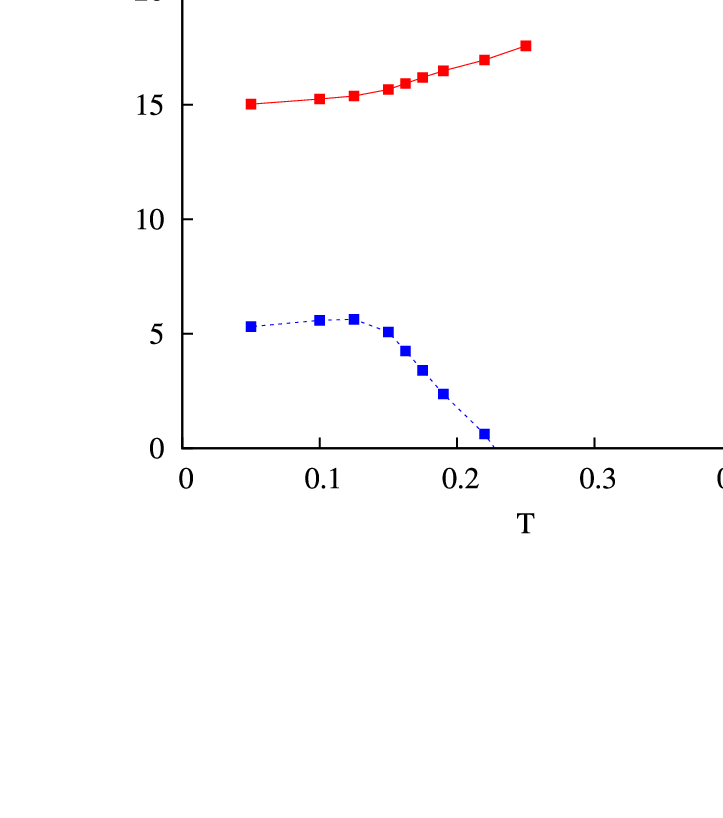
A test case: a binary soft-sphere system - To test our scheme we performed an explicit computation of the shear modulus of the standard binary mixture of particles with soft-core interactions [16]. The Kauzmann temperature of this system is $T_{\rm K}\simeq 0.14$ [8] while the dynamical (MCT) transition temperature is $T_{\rm c}\simeq 0.22$ [17]. In Fig. 2 we show the result for the case of density $\rho=1$. To evaluate $m^{*}$ and the radial distribution function $g_{*}(r)$ at $T^{*}$, we performed the cloned liquid computation using the binary HNC approximation [8].

The evaluation of various terms in Eq. (6) is done as follows. The Born term and $J_{2}$ involve only 2-point functions so that they can be evaluated easily using $g_{*}(r)$. We evaluate $J_{1}$ by $J_{1}=-2\frac{A}{m}\int d^{3}rg_{*}(r)\beta^{*}|\nabla\sigma|^{2}(r)-2\frac{A}{m}\int d^{3}r_{1}d^{3}r_{2}g({\bf r}_{1})g({\bf r}_{2})g({\bf r}_{12})\beta^{*}\nabla\sigma({\bf r_{1}})\cdot\nabla\sigma({\bf r_{2}})$ where we made a chain approximation in order to approximate the three-point correlation function by a product of two-point terms, an approximation which is reasonable at high densities. The evaluation of $J_{3}$ involves a connected 4-point function which is expected to be smaller than the other terms and we have neglected it at present.

As shown in Fig 2, the plateau-modulus $\hat{\mu}$ strongly depends on the temperature. Remarkably, it continuously crosses $0$ at a temperature very close to $T_{c}$ determined by direct numerical simulations [17]. Furthermore the cage size $A$ is found to be still very small ($10^{-2}$) at this temperature, which justifies our use of the first order small cage expansion. Our result of a plateau shear modulus emerging continuously below $T_{\rm c}$ disagrees with the conventional MCT [6], which predicts that the shear-modulus jumps discontinuously to a finite value at $T_{\rm c}$ from the liquid side. Our result means that the density field is frozen at $T_{c}$ as the MCT predicted, but the system is just marginally stable there [12], a picture which is consistent with the energy landscape picture of the RFOT [19, 18, 20, 21, 22]. For the visco-elastic measurements, this continuous transition suggests a power law behaviour $G^{\prime}(\omega),G"(\omega)\propto\omega^{\lambda}$.

Intermittency of static shear response - Our results have a natural interpretation within a mean-field picture. They suggest the following “intermittent” nature of static shear response below $T_{\rm K}$ at mesoscopic scales such that the system size $N$ is large but finite. Within mean field, the parameter $m=m^{*}(T)\simeq T/T_{\rm K}$ obtained in the cloned liquid approach is naturally interpreted as the Parisi parameter of the 1 step replica symmetry breaking (1RSB) Ansatz for the glass phase.

As shown in Fig. 1, the interpretation at the mean field level is that of a free-energy landscape $F(\gamma)$ which may be viewed as sequence of parabola with curvature $\hat{\mu}$ (plateau-modulus) along the $\gamma$-axis, matching with each other at yield points [23]. Below $T_{\rm K}$, the static response to shear is dominated by intra-state response with occasional inter-state response when passing the yield points.

This picture is analogous to the mesoscopic response in mean-field spin-glass models [24]. Here $\gamma$ plays the role of the external magnetic field $h$ in spin glasses, which exhibit step-wise increase of magnetization $m(h)$ along $h$-axis. The drops of the stress passing the yield points corresponds to steps of the magnetization. At a given $\gamma$, each metastable state has a random free-energy $f_{\alpha}$ and a random stress $\langle\sigma\rangle_{\alpha}$ so that the increase of $\gamma$ induces level crossings between low-lying states.

The distribution of the stress may be modeled by a Gaussian distribution with zero average and variance $\Delta/\sqrt{N}$. From the correspondence with the spin-glass problem [24] we expect the typical spacing between the yield points to scale as $\delta\gamma_{\rm s}\sim T_{\rm K}/(\Delta\sqrt{N})$ and the width of thermal rounding of the yield points to scale as $\delta\gamma_{\rm w}\sim T/(\Delta\sqrt{N})$. Here the parameter $\Delta$ is fixed as $\beta\Delta^{2}=\hat{\mu}/m$ in order to satisfy the condition that the total shear-modulus, including the inter-state shear-modulus, becomes zero on average. At low temperatures, if we choose a value of $\gamma$ randomly, most of the time we will observe the plateau modulus $\hat{\mu}$ which is positive, and occasionally, with probablity $\delta\gamma_{\rm w}/\delta\gamma_{\rm s}\sim T/T_{\rm K}$, we will find a negative shear-modulus.

Discussion - Our computations predict a non-zero plateau-modulus $\hat{\mu}$ at all temperatures below the dynamical transition temperature $T_{\rm c}$, including in the low temperature regime [25]. They also give a natural way to compute this dynamical transition temperature within the cloned liquid theory, offering an alternative to the MCT computation. This plateau modulus should be observable dynamically on time scales smaller than the $\alpha$ relaxation time $\tau_{\alpha}$. Therefore one expects it to be seen, on all laboratory time scales, at all temperatures below the glass transition temperature (where the $\alpha$ relaxation time becomes larger than $10^{3}$s).

The prediction of intermittent shear response in mesoscopic samples should also be amenable to experimental tests. It is supposed to take place even at temperatures higher than $T_{\rm K}$ at the length and time scales of the so-called mosaic states proposed by the RFOT [4, 5] because each mosaic is subjected to a random pinning field provided by surounding mosaics.

Acknowledgment We thank Giulio Biroli, Jean-Philippe Bouchaud, Song-Ho Chong, Silvio Franz, Jorge Kurchan, Anael Lemaître, Kunimasa Miyazaki, Michio Otsuki and Tommaso Rizzo for useful discussions. This work is supported by a Triangle de la physique grant number 117.

References

- [1] C. A. Angell, Science 267, 1924 (1995).
- [2] C. Maggi, B. Jakobsen, T. Christensen, N. B. Olsen, and J. C. Dyre, J. of Phys.Chem. B 112, 16320 (2008).
- [3] T. G. Mason, Martin-D. Lacasse, Gary S. Grest, Dov Levine, J. Bibette, D. A. Weitz, Phys. Rev. E 56, 3150 (1997).
- [4] T. R. Kirkpatrick, D. Thirumalai, and P. G. Wolynes, Phys. Rev. A 40, 1045 (1989).
- [5] M.P. Eastwood and P.G. Wolynes, Europhys. Lett. 60, 587 (2002). J-P. Bouchaud, G. Biroli, J. of Chem. Phys. 121, 7347 (2004). G. Biroli, J. P. Bouchaud, A. Cavagna, T. S. Grigera, and P. Verrocchio, Nature Physics 4, 771 (2008).
- [6] W. Götze, in: J. P. Hanssen, D. Levesque, J. Zinn-Justin (Eds.), Liquids, Freezing and Glass transition, North Holland, Amsterdam, 1991 p.287.
- [7] M. Mézard and G. Parisi, Phys. Rev. Lett. 82 747 (1999) and J. of Chem. Phys, 111 1076 (1999).
- [8] B. Coluzzi, M. Mézard, G. Parisi and P. Verrochio, J. of Chem. Phys, 111 9039 (1999).
- [9] G. Parisi and F. Zamponi, arXiv:0802.2180 to appear in Rev. Mod. Phys.
- [10] S. Franz, J. Stat. Mech. (2005) P04001
- [11] F. Sausset, G. Biroli and J. Kurchan, “Do solids flow?”, arXiv:1001.0918
- [12] M. Otsuki and S.-i. Sasa, J. Stat. Mech. L10004 (2006).
- [13] D. R. Squire, A. C. Holt, and W. G. Hoover, Physica, 42, Issue 3, p.388 (1969).
- [14] Details of the derivations will be published elsewhere.
- [15] A.W. Kauzmann, Chem.Rev 43 (1948) 219.
- [16] B. Bernu, J. P. Hansen, Y. Hiwatari, and G. Pastore, Phys. Rev. A 36, 4891 (1987).
- [17] J. N. Roux, J. L. Barrat, and Hansen, J. of Phys.: Condensed Matter 1, 7171 (1989).
- [18] J. Kurchan and L. Laloux, Journal of Physics A: Mathematical and General 29, 1929 (1996)
- [19] S. Franz and G. Parisi, Phys. Rev. Lett. 79, 2486 (1997),
- [20] S. Franz and G. Parisi, J. of Phys.: Condensed Matter 12, 6335 (2000).
- [21] T. S. Grigera, A. Cavagna, I. Giardina, and G. Parisi, Phys. Rev. Lett. 88, 055502 (2002).
- [22] L. Berthier, J.-L. Barrat and J. Kurchan, Phys. Rev. E61, 5464 (2000).
- [23] J-P. Bouchaud and M. Mézard. J. Phys. A 30, 7997 (1997).
- [24] H. Yoshino and T. Rizzo Phys. Rev. B 77, 104429 (2008).
- [25] C. Maloney and A. Lemaître, Phys. Rev. Lett. 93, 195501 (2004), F. Leonforte, R. Boissière, A. Tanguy, J. P. Wittmer, and J.-L. Barrat, Phys. Rev. B 72 224206 (2005).