A concordance invariant from the Floer homology of -surgeries
Abstract.
We discuss a concordance invariant constructed from Heegaard Floer homology “correction terms” and surgeries on knots.
1. Introduction
Given a closed oriented three-manifold with torsion structure, the associated Heegaard Floer homology groups come with absolute –gradings; see Ozsváth–Szabó [OS06]. This allows one to define numerical invariants of three-manifolds, the so-called “correction terms” or “–invariants”. Specifically, suppose is a rational homology three-sphere. Then Ozsváth and Szabó define (the correction term) to be the minimal degree of any non-torsion class in coming from 11 1 There are correction terms for three-manifolds with positive first Betti number, but we do not discuss them at the moment.. This invariant is analogous to the monopole Floer homology –invariant introduced by Frøyshov [Frø96]. If only has a single structure (ie if is an integer homology sphere), then we denote by just . The –invariants satisfy some useful properties, according to the following theorem of Ozsváth and Szabó:
Theorem 1.1 (Ozsváth–Szabó [OS04a]).
Let be an oriented rational homology three-sphere. Its correction terms satisfy:
- (1)
Conjugation invariance
- (2)
If is an integral homology three-sphere and is the oriented boundary of a negative-definite four-manifold then .
In fact, item 2 follows from a more general statement, Proposition 3.2, and the following theorem of Elkies.
Theorem 1.2 (Elkies [Elk95]).
Let be a negative-definite unimodular bilinear form over . Denote by the set of characteristic vectors for Q, ie the set of vectors satisfying
for all . Then,
with equality if and only if the bilinear form is diagonalizable over .
Also, can be a disjoint union of rational homology three-spheres, in which case Theorem 1.1 (together with Theorem 1.2) implies:
Corollary 1.3 (Ozsváth–Szabó [OS04a]).
Let and be oriented rational homology three-spheres. Then
- (1)
Let denote the manifold with opposite orientation, then
- (2)
If is rational homology cobordant to , then
- (3)
If and are integral homology three-spheres and is a negative-definite cobordism from to , then
- (4)
If bounds a rational homology four-ball, then .
Heegaard Floer homology --invariants have been used to give restrictions on intersection forms of four-manifolds which can bound a given three-manifold (for instance, Ozsváth and Szabó reproved Donaldson’s diagonalization theorem using correction terms). They have also been used to define concordance invariants of knots22 2 Heegaard Floer theory has led to other concordance invariants, most notably the invariant (see Ozsváth–Szabó [OS03b] and Rasmussen [Ras03]).. For instance, Manolescu and Owens [MO07] used the –invariants of the branched double cover of a knot to produce concordance invariants (see also Grigsby, Ruberman, and Strle [GRS08], Jabuka [Jab], and Jabuka and Naik [JN04]). In this paper, given a knot in the three-sphere, we show that is a concordance invariant of and examine some of its properties. Occasionally we denote this invariant by . Note that one could also study , but these invariants are determined by the since where denotes the mirror of . We also establish a “skein inequality” reminiscent of a property of the knot signature. Specifically,
Theorem 1.4.
Given a diagram for a knot with distinguished crossing , let and be the result of switching to positive and negative crossings, respectively, as in Figure 2. Then
for any field . Here, denotes the correction term of computed from Floer homology with coefficients in .
Indeed, we expect that the restriction that the coefficients are taken in a field could be relaxed to include –coefficients, but our proof only holds for field coefficients. The invariants also give rise to four-ball genus bounds. Specifically, we have the following:
Theorem 1.5.
Let be a knot in the three-sphere. Then
where denotes the smooth four-ball genus of .
Again, we expect that this should hold for Floer homology with any coefficients, but our proof is special to –coefficients. Theorem 1.5 should be compared to the following theorem of Frøyshov:
Theorem 1.6 (Frøyshov [Frø04]).
Let be an oriented homology three-sphere and a knot in of “slice genus” . If is the result of –surgery on then
Here is Frøyshov’s instanton Floer homology –invariant and the “slice genus” is defined to be the smallest non-negative integer for which there exists a smooth rational homology cobordism from to some rational homology sphere and a genus surface such that . It is not clear to the author whether this definition agrees with the usual one for . In light of the conjectural relationship and Theorem 1.6, we suspect that the inequality in Theorem 1.5 is in general weaker than the –invariant inequality.
Finally, using the theory of Ozsváth–Szabó [OS04b] and Rasmussen [Ras03], we observe how one can algorithmically compute if one knows the filtered chain homotopy type of the knot complex . A computer implementation of this algorithm is discussed.
1.1. Further questions
What is the relationship between the correction terms of –surgeries on a knot and the Ozsváth–Szabó, Rasmussen invariant? From the discussion in Section 5, it seems likely that , but as of the time of this writing a proof remains elusive. Of course if this were the case, then the genus bound, Theorem 1.5, would follow immediately from the inequality (see Ozsváth and Szabó [OS03b] for a discussion).
1.2. Organization
This paper is organized as follows. In Section 2, we discuss basic properties of , including its invariance under concordance. In Section 3 we give a proof of the skein inequality, Theorem 1.4. In Section 4 we prove Theorem 1.5. Finally in Section 5 we discuss an algorithm to compute given the knot complex as well as a computer implementation of this algorithm.
1.3. Acknowledgement
The author would like to thank his PhD supervisor, Peter Ozsváth for suggesting the problem as well as invaluable guidance over the years. He would also like to thank Maciej Borodzik, Kim Frøyshov, Matt Hedden, Adam Levine, and Danny Ruberman for helpful conversations.
2. The invariant
Proposition 2.1.
is a concordance invariant.
Proof.
It is simple to see that if is smoothly slice: bounds the four-manifold obtained by attaching a –framed two-handle along to the four-ball. This four-manifold has second homology generated by a sphere of square . By blowing this down, we see that bounds a rational homology four-ball. By item 4 of Corollary 1.3, it follows that . It is just slightly more work to see that if and are smoothly concordant, then : the concordance gives us a smoothly embedded annulus (here ) with and , . Attach a two-handle to with framing along to give a four-manifold (see Figure 1). Consider a small regular neighborhood of the core disk of this two-handle union a regular neighborhood of the annulus . This gives cobordisms and such that . Notice that is just , a –framed two-handle attached along to a thickened . It follows that and (this last fact can be seen from the Mayer–Vietoris sequence applied to the decomposition : ). Applying item 2 of Corollary 1.3 to shows that . ∎
In fact, the basic topological fact that if knots , are concordant then is homology cobordant to used in the previous argument follows from a more general fact due to Gordon [Gor75]: If two knots and are concordant, then for any , we have a homology cobordism . As pointed out by several people, this implies that for each rational , we get concordance invariants . It is natural to ask about the independence of these invariants.
2pt \pinlabel at 56 82 \pinlabel at -8 37 \pinlabel at 60 -8 \pinlabel at 126 11 \pinlabel at 150 67 \endlabellist

In general, calculating –invariants is quite challenging. However, in certain cases explicit formulae exist. For instance, let be an alternating knot. Then in [OS03a], Ozsváth and Szabó prove that
| (1) |
where is the ceiling function and denotes the knot signature (see also Rasmussen [Ras02]). This formula shows that the concordance invariants do not give group homomorphisms from the smooth concordance group to : take the knot where denotes the right-handed trefoil and denotes the left-handed trefoil. This knot is slice and hence has vanishing but and . Explicit formulae for –invariants also exist in the case of certain plumbed three-manifolds; see Ozsváth–Szabó [OS03c]. In another direction, since torus knots admit lens space surgeries, one may use Ozsváth–Szabó [OS05, Theorem 1.2] to calculate for torus knots.
It may be worth noting that Equation 1 does not hold for all knots. For instance, the –torus knot has signature and .
The non-additivity of can be used to detect relations or establish linear independence in the smooth concordance group, . For example, recall that , , and (here, denotes the Rasmussen concordance invariant of [Ras]). It is also the case that , , where here denotes the –torus knot. It follows that for any among , , or . However, this knot is not slice, since , a fact which can be verified with our program dCalc.
3. Skein relations
Recall the axiomatic characterization of the knot signature found by Giller (see also Murasugi [Mur96]).
Theorem 3.1 (Giller [Gil89]).
Suppose that is a knot (but not a link) and is a diagram for . Then can be determined from the following three axioms:
- (1)
If is the unknot then .
- (2)
- (3)
If is the Conway-normalized Alexander polynomial of , then
2pt \pinlabel at 19 -8 \pinlabel at 126 -8 \endlabellist

These axioms of course cannot hold for the invariant , but Theorem 1.4 does give us an analogue of Theorem 3.1, item (2).
In light of the the axiomatic description of , it is an interesting question to calculate modulo 2. If one could achieve this, it might then be possible to give a completely algorithmic description of .
2pt \pinlabel at 44 18 \pinlabel at 45 46 \pinlabel at 18 -8 \pinlabel at 151 18 \pinlabel at 152 46 \pinlabel at 127 -8 \endlabellist

2pt \pinlabel at 86 32 \pinlabel at 100 -8 \endlabellist

We now return to the proof of Theorem 1.4.
Proof of Theorem 1.4.
Step 1: :
Given a knot with diagram and a distinguished crossing, we have cobordisms and given by the Kirby diagrams in Figure 3. We claim that for . We argue this for , the argument for being analogous. fits into a four-manifold where is obtained by attaching a –framed two-handle along to the four-ball. Clearly and Consider the Mayer–Vietoris sequence applied to the decomposition . In this case, , an integral homology three-sphere. So we have showing that . We may even find a torus in which generates as in Figure 4. We claim that (likewise, for we have can find a torus of square generating ). of course sits inside the larger cobordism . Let be an ordered basis of coming from the two two-handles (more specifically, is the homology class of the core disk of the two-handle attached to capped off by a Seifert surface, and is the homology class of the core disk of the two-handle attached to the –framed knot in Figure 4 capped off with a Seifert surface pushed slightly into the four-ball). With respect to this basis, we see that the intersection form of is given by the matrix
By Figure 4, it is clear that and . Therefore and . By item 3 of Corollary 1.3 it follows that
Step 2: :
By a similar argument to the previous, we see that the cobordism has second homology generated by a torus of square . Taking an internal connected sum of with a regular neighborhood of , , we get cobordisms and such that . Here denotes the boundary of a regular neighborhood of the surface in . This is of course a circle bundle over the two-torus with Euler number (it is also a torus bundle over the circle with reducible monodromy). It may be realized as –surgery on the Borromean rings, which we denote by . Clearly for otherwise we would have a surface with positive square in which does not intersect the generating torus . Similarly, we have that . Notice that deformation retracts onto the wedge and hence has euler characteristic . Since and ( is a three-manifold) we see that . Therefore the cobordism has , (here denotes the signature of the intersection form of ), and for all structures . By the formula for grading shifts in Heegaard Floer homology (see Ozsváth and Szabó [OS06]), it follows that the maps on Floer homology associated with this cobordism have grading shift
Before continuing with –invariant calculations, we pause to recall some constructions in Heegaard Floer theory for manifolds with . In this case, there is a natural action of the exterior algebra on all versions of Floer homology . Under this action, elements of drop relative gradings by one. As an example, let denote the graded abelian group supported in grading . Under the graded isomorphism , the action of the circle factor is given by and .
A three-manifold with torsion structure is said to have standard if there is a graded isomorphism of –modules
| (3) |
where the action of on the right hand side is given by contraction on
. Here is graded by the requirement that and the fact that drops gradings by 1. For example, has standard for any as does any three-manifold with by a theorem of Ozsváth and Szabó [OS04c, Theorem 10.1]. For three-manifolds with standard there is a “bottom-most” correction term, denoted , which is defined to be the smallest grading of any non-torsion element coming from an element which lies in the kernel of the action by . Notice that, in contrast to “ordinary” correction terms, it is not true in general that (for instance, take ). The correction terms give restrictions on intersection forms of negative semi-definite four-manifolds bounding a given three-manifold according to:
Proposition 3.2 (Ozsváth–Szabó [OS04a]).
Let be a closed oriented three-manifold (not necessarily connected) with torsion structure and standard . Then for each negative semi-definite four-manifold which bounds so that the restriction map is trivial, we have the inequality
for all structures over whose restriction to is .
Returning to the proof of Theorem 1.4, recall that we have a cobordism
with . Therefore for all structures on . Note also that : consider the Mayer–Vietoris sequence applied to :
(recall that and that ; denoting homotopy equivalence). Applying Proposition 3.2 to we see that:
| (4) |
Claim 3.3.
.
Notice that this would imply Theorem 1.4. To prove the claim, recall that in [OS04a], Ozsváth and Szabó calculated that , supported completely in the unique torsion structure. This implies that , and by the long exact sequence
it follows that where denotes the graded -module graded so that multiplication by is degree and lies in grading . Writing for some torsion module ( is called the reduced Floer homology of , and is also written ), we get that , by item 1 of Corollary 1.3. By the long exact sequence
we get that for some torsion -module where here denotes the graded –module graded so that multiplication by is degree and lies in grading . Using the formula
from Ozsváth–Szabó [OS04c], if we use Floer homology with field coefficients , we have:
(since is a principal ideal domain). It follows that
for some torsion module . Therefore
and we have shown that
4. Genus bounds
Proof of Theorem 1.5.
Step 1: :
Let , the smooth four-ball genus of , ie the minimum genus of any smooth surface smoothly embedded in the four-ball with boundary . Now attach a –framed two-handle to the four-ball along the mirror of , denoted . Now delete a small ball from the four-ball. This gives a negative definite cobordism whose second homology is generated by a surface of genus and square . By item 3 of Corollary 1.3 and the fact that we get that . Since , we are done.
Step 2: :
Similar to the previous paragraph, by removing a small ball from the four-ball and then attaching a –framed two-handle to the boundary three-sphere along , we obtain a cobordism
which contains a genus surface of square , . Let denote an euler number circle bundle over a surface of genus . In the notation of the previous section, we have . is of course homeomorphic to the boundary of a regular neighborhood of . Similar to previous discussions, by taking an internal connected sum we get a pair of cobordisms
and
with . Notice that the oriented manifold has standard by Ozsváth–Szabó [OS04a, Propositions 9.3 and 9.4] since we may connect it via a negative-definite cobordism to , which has standard . Applying Proposition 3.2, we see that
| (5) |
Theorem 1.5 would follow if we could show that . Indeed, we show this in Lemma 4.2. The calculation of follows quickly from the machinery of [OS08], which we recall in Section 4.1.∎
4.1. Review of the integer surgery formula
In this section we review the essential details needed to state Ozsváth and Szabó’s “integer surgery formula,” referring the reader to [OS08] for more details. Suppose is a three-manifold with torsion and suppose that is a null-homologous knot. Fixing a Seifert surface for , we can assign to its knot Floer homology , a –bifiltered chain complex well-defined up to filtered chain homotopy type as described in Ozsváth–Szabó [OS04b]. This is an abelian group generated by tuples for integers and intersection points coming from a particular Heegaard diagram for (see Ozsváth–Szabó [OS04b] for a proper discussion). This group comes with an absolute –grading as well as an action by . There is an identification of structures over which are –cobordant to over a certain cobordism with . For , let denote the corresponding summand of .
Let and , the latter being identified with . There are maps
and
defined as follows: is just the projection while is the projection followed by an identification (induced by multiplication by ) followed by a “natural” homotopy equivalence . The map is obtained by the handleslide invariance of Heegaard Floer homology and is natural in the sense that the induced map on homology is independent (up to a sign) of a chosen sequence of handleslides. Set
and:
Define
by
Assign gradings to , as follows. Under the identification , we map homogeneous elements of degree in to homogeneous elements of of degree
| (6) |
or
| (7) |
It is then possible to assign gradings to the which are consistent with their natural relative –gradings in such a way that the maps and are homogeneous of degree . With this all in place, we may now state the “integer surgery formula” of [OS04a]:
Theorem 4.1 (Ozsváth–Szabó [OS04a]).
Fix a structure over whose first Chern class is torsion, a null-homologous knot, and a non-zero integer. For each , the mapping cone of
is isomorphic, as a relatively graded –module, to . In fact, this isomorphism is homogeneous of degree where
for and for .
Recall that the mapping cone of the map has underlying group and differential
Also, when , and there is no additional choice of . When this is satisfied, we write simply instead of .
4.2. A useful computation
Lemma 4.2.
For as before, we have
where denotes the –invariant of as computed from Floer homology with coefficients in .
Proof.
The oriented manifold may be obtained as –surgery on the knot (the “Borromean knot”) shown in Figure 5.
2pt \pinlabel at 50 90 \pinlabel at 152 90 \pinlabel at 76 70 \pinlabel at 101 19 \pinlabel at 183 64 \pinlabel at 101 -6 \endlabellist

We start with the calculation for . Since the second homology of is generated by embedded tori, the adjunction inequality (Ozsváth–Szabó [OS04c, Theorem 7.1]) implies that is non-zero only in the unique torsion structure . The knot Floer complex for the Borromean knot is calculated in Ozsváth–Szabó [OS04b] to be
with –bifiltration given by:
| (8) |
Furthermore, the group is supported in grading and all differentials vanish (including all “higher” differentials coming from the spectral sequence ).
Under the above identification, and the identification , the action of on is given explicitly by
| (9) |
where denotes contraction. Since , this action may be viewed as a reflection of the fact that is standard.
The only presumably non-combinatorial ingredient in the integer surgery formula (once the complex is at hand) is the necessary explicit identification of the natural homotopy equivalence . The homotopy takes a particularly simple form for Floer homology with coefficients in , with which we work for the remainder of this section. The description of is as follows:
Proposition 4.3 (Ozsváth–Szabó [OS04a]).
For the Borromean knot , the natural homotopy equivalence sends to .
Interestingly, the above proposition does not hold for Floer homology with coefficients in (see Jabuka–Mark [JM08a] for a description).
We picture the complex as below:
For simplicity of discussion, we currently restrict to the case of . In this case, a piece of looks like Figure 6.
2pt
at 10 70 \pinlabel at 36 52 \pinlabel at 36 37 \pinlabel at 36 22 \pinlabel at 51 67 \pinlabel at 51 52 \pinlabel at 51 37 \pinlabel at 66 67
at 100 70 \pinlabel at 126 52 \pinlabel at 126 37 \pinlabel at 126 22 \pinlabel at 141 67 \pinlabel at 141 52 \pinlabel at 141 37 \pinlabel at 156 67
at 190 70 \pinlabel at 216 52 \pinlabel at 216 37 \pinlabel at 216 22 \pinlabel at 231 67 \pinlabel at 231 52 \pinlabel at 231 37 \pinlabel at 246 67
at 10 178 \pinlabel at 6 130 \pinlabel at 21 130 \pinlabel at 21 145 \pinlabel at 36 160 \pinlabel at 36 145 \pinlabel at 36 130 \pinlabel at 51 175 \pinlabel at 51 160 \pinlabel at 51 145 \pinlabel at 66 175
at 100 178 \pinlabel at 111 145 \pinlabel at 126 160 \pinlabel at 126 145 \pinlabel at 126 130 \pinlabel at 141 175 \pinlabel at 141 160 \pinlabel at 141 145 \pinlabel at 156 175
at 190 178 \pinlabel at 216 160 \pinlabel at 216 145 \pinlabel at 216 130 \pinlabel at 231 175 \pinlabel at 231 160 \pinlabel at 231 145 \pinlabel at 246 175
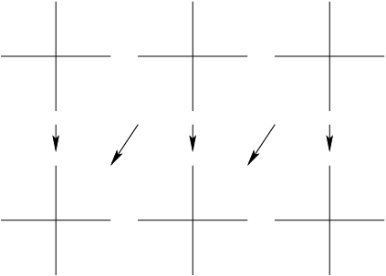
We claim that the correction terms of can be read off from Figure 6. Indeed, writing and , consider the element . Since
it follows that is a cycle. We claim that is also not a boundary. Indeed, suppose that for some . Then would necessarily have either a non-zero component in or a non-zero component in . In either case, a simple diagram chase shows that cannot be extended to a cycle in (ride the zig-zag and notice that would have infinitely many non-zero components in ).
It is, however, the case that is a boundary: the element maps to it under .
Using similar reasoning, one can show that the elements
all represent generators for the four “towers” of . According to the grading formula, Equation 7, these elements have grading 1,0,0, and 1, respectfully. It follows that:
where here we are using a slight abuse of notation: now denotes (for the previous definition of ) and Floer homology with –coefficients is understood. Further, according to the action, Equation 9, it follows that (alternatively this follows since has standard via Equation 3). Although we already knew how to compute this, the advantage of this calculation is that the reasoning generalizes to arbitrary . Indeed, for general one can check that the intersection
gives representatives for generators of the “towers” of . Using the grading formula, Equation 7, it follows that:
By the action formula, Equation 9, (or the fact that is standard) it follows that
Calculating is similar. In that case, the generators of the intersection
may be extended (in one step) to representative cycles for the homology . Using Equation 6 one calculates that:
The action formula, Equation 9, gives
| (10) |
proving Lemma 4.2∎
An alternative approach to the calculation of the correction terms of –surgery on the Borromean knot of genus is the integer surgery exact sequence, together with Jabuka-Mark’s calculation of the Floer homology of [JM08b]. It is interesting to note that has been calculated in Ozsváth–Szabó [OS04b].
In fact, the methods in this section give the following:
Theorem 4.4.
Let be a smooth, simply-connected, compact, oriented four-manifold with a homology sphere as boundary with and . Let be a closed surface of genus and self-intersection . Then
5. Computations
In this section we discuss an algorithm to compute the invariants assuming we know the filtered chain homotopy type of the knot complex of Ozsváth–Szabó [OS04b]. We also discuss a computer implementation of this algorithm. The algorithm we use is based on the theory of Ozsváth–Szabó [OS04b, OS04a], and Rasmussen [Ras03] and has three steps:
- (1)
- (2)
Use exact sequences to compute the correction terms of .
- (3)
Use a simple relation between the correction terms of and the correction terms of .
We describe the steps in reverse order. Recall from [OS04a] that for a closed oriented three-manifold with , there are two correction terms , where is the minimal grading of any non-torsion element in the image of in with grading modulo 2. Then step 3 follows from Ozsváth–Szabó [OS04a, Proposition 4.12 ] which states that
| (11) |
and
| (12) |
This proposition is an easy consequence of the fact that is standard and the exact sequence, Equation 2.
For step 2, recall the integral surgeries long exact sequence (see Ozsváth–Szabó [OS04c, Theorem 9.19]; [OS04a] for the graded version). Let be a knot in an integral homology three-sphere and a positive integer. Then we get a map
and a long exact sequence of the form
| (13) |
where
Moreover, the component of in the above exact sequence which takes into the -component of has degree , while the restriction of to the –summand of has degree . It follows from this exact sequence that . To get , we may use a similar exact sequence for negative surgeries.
is finitely generated as a complex over . It comes with an absolute –grading and a –bifiltration. Generators are written for integers and intersection points in a Heegaard diagram for . The –action is given by . We picture these complexes as graphs in the plane, as in Figure 7 (1). Dots represent generating ’s while arrows represent differentials. The absolute grading is (basically) pinned down by the fact that if we consider the “–slice” quotient complex , then its homology (which is guaranteed to be a single copy of —the generator of ) is supported in grading , the fact that the –action drops absolute grading by , and the fact that differentials drop grading by 33 3 This is actually not quite true: not all vertices appearing in the complex are related to the generator of by a sequence of –maps and differentials. To grade these remaining vertices, we have to go back to the Heegaard diagram. However, for the purpose of computing –invariants, we do not need to look at these at all..
In order to accomplish step 1, we use the following theorem of Ozsváth–Szabó, Rasmussen (see, for instance, Ozsváth–Szabó [OS04b, Corollary 4.3])
Proposition 5.1 (Ozsváth–Szabó [OS04b], Rasmussen [Ras03]).
Let be a knot in the three-sphere. Then there exists a positive integer with the property that for all we have that
where
Similarly,
where
In fact, we can take where is the knot genus.
We can pick off the correction terms from this theorem: we know that
so choose a class which generates this homology as a –module. Look at a sufficiently negative –power of this generator. This generates the “tower” of . All one has to do is start taking –powers of and see when they vanish in homology. The grading of the last-surviving –power of is (after the grading shift). A similar story allows one to compute .
Write , the “unshifted” correction term of the group . Putting together the previous discussion, by the exact sequence, Equation 13 we have:
Using Equation 11 we get:
ie
| (14) |
We now discuss how to teach a computer to do step 1. In fact, we implemented this in C++ in a program called dCalc (beta). The source code is available at
As previously mentioned, is finitely generated as a complex over . By a symmetry property of the knot Floer homology, we may assume that the corresponding graph is symmetric about the line . With such a graph at hand, we choose a generating set which is
- (1)
Minimal: no smaller subset of it generates .
- (2)
In the first quadrant, and .
- (3)
As close to the origin as possible.
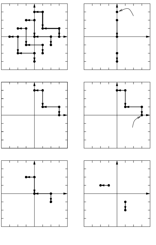
(See Figure 7 for an example). We started with a digraph data structure to represent the complexes. Vertices were marked with –bifiltration levels and could be marked with gradings. Vertices are also marked to keep track of bases. The first step was to fill in the gradings. For this we needed to compute the “–slice” described before. This is determined by a finite number of –translates of our chosen generating set. Once we find the generator of , it is a problem in graph traversal to fill in (most of—see footnote 3) the other gradings. Our chosen generating set will necessarily have –dimensional homology (over ) and its generator will have a grading computed from the graph traversal. This generator maps to a generator of . To compute , we start by taking a finite piece of the complex (more specifically, take our chosen generating set and start hitting it by —at some point it will disappear out of the “hook” region . Take only those images which appear in the hook). In the graph implementation, this just involves shifting filtration levels and throwing away some vertices as they exit the hook. Now take the generator and start pushing it down by until it dies in homology. Its grading just before it dies is , by Equation 14. To compute , one runs a similar story, but instead of using the “hook region” , one uses the first quadrant .
Since one knows how knot complexes behave under connected sum of knots (tensor product over ; see Ozsváth–Szabó [OS04b, Theorem 7.1] for the precise formulation), we implemented this as well, allowing users to compute correction terms of surgeries on connected sums of knots.
5.1. A few examples
In this section, Floer homology with mod-2 coefficients is understood. Figure 7 shows an example of the algorithm described in Section 5. Here, we are given the knot complex for the –torus knot, which was computed in Ozsváth–Szabó [OS04a, Section 5.1] or by [OS05, Theorem 1.2].
2pt \pinlabel1. Find minimal generating. at 65 308 \pinlabel graph (shown in bold). at 65 296 \pinlabel2. Find generator of “-slice.” at 236 306 \pinlabelHere it is! at 251 413 \pinlabel3. Fill in gradings. at 45 145 \pinlabelThis will do. at 266 188 \pinlabel4. Find a generator of at 216 150 \pinlabel homology. at 216 139 \pinlabelNot quite at 106 30 \pinlabeldead yet… at 122 18 \pinlabel5. Start pushing generator down at 80 -6 \pinlabel by until it dies in the at 70 -18 \pinlabel “hook” region, . at 65 -30 \pinlabelRIP at 248 18 \pinlabel6. Grading before death was at 236 -6 \pinlabel at 236 -18 \pinlabel at 145 380 \pinlabel at 66 450 \pinlabel at 52 273 \pinlabel at 92 278 \pinlabel at 74 234 \pinlabel at 122 248 \pinlabel at 113 213 \endlabellist
As another example, consider the right-handed trefoil . This knot has knot Floer homology given by
Here, denote the Alexander and Maslov gradings, respectfully. Since we know there is a spectral sequence, induced by the Alexander filtration on , converging to (supported in grading 0), it follows that the page of this spectral sequence is given in Figure 8.
2pt \pinlabel at 30 39 \pinlabel at 8 19 \pinlabel at 48 55 \pinlabelMaslov at 25 -3 \pinlabelAlexander at -35 55 \endlabellist

By the symmetry of , it follows that is generated as a –module by the complex in Figure 9.
2pt \pinlabel at 47 43 \pinlabel at 47 13 \pinlabel at 15 43 \pinlabel at 16 3 \pinlabel at 2 13 \endlabellist

which shows that , a fact which more readily follows from Equation 1.
Next, consider the figure eight knot, . This knot has knot Floer homology
Again, by considering the spectral sequence , it follows that the page of this spectral sequence is given Figure 10.
2pt \pinlabel at 33 35 \pinlabel at 61 66 \pinlabel at 5 11 \pinlabelAlexander at -33 37 \pinlabelMaslov at 35 78 \endlabellist

It follows that is generated as a –module by the complex shown in Figure 11.
2pt \pinlabel at 52 52 \pinlabel at 52 24 \pinlabel at 24 24 \pinlabel at 24 52 \pinlabel at 14 14 \pinlabel at 3 24 \pinlabel at 23 5 \endlabellist

2pt \pinlabel at 169 197 \pinlabel at 143 171 \pinlabel at 117 144 \pinlabel at 93 122 \pinlabel at 63 91 \pinlabel at 35 62 \pinlabel at 7 35 \pinlabel at 153 190 \pinlabel at 129 165 \pinlabel at 102 140 \pinlabel at 75 112 \pinlabel at 45 81 \pinlabel at 18 54 \pinlabel at 170 170 \pinlabel at 147 147 \pinlabel at 120 120 \pinlabel at 93 93 \pinlabel at 66 66 \pinlabel at 36 36 \pinlabel at 9 9 \pinlabel at 166 157 \pinlabel at 139 128 \pinlabel at 112 101 \pinlabel at 84 75 \pinlabel at 56 45 \pinlabel at 29 19 \endlabellist

Here, we see a single isolated at the origin plus a null-homologous “box”. It is then easy to see that (again, this follows more quickly from Equation 1).
Recall that while the Kinoshita–Terasaka knot is smoothly slice, it is currently unknown if its Conway mutant is smoothly slice (though it is topologically slice since it has trivial Alexander polynomial, by a result of Freedman [FQ90, Fre83]). Indeed, we currently show that , showing that our invariant gives no information. In [BG], Baldwin and Gillam calculated the knot Floer homology polynomial44 4 The knot Floer homology polynomial of a knot is defined to be . of to be:
| (15) |
Similar to previous computations, it follows that the term of the spectral sequence is forced to be as in Figure 12. From this, it follows that can be computed by a complex generated as a –module with a single isolated at the origin plus a collection of null-homologous “boxes”. As in the computation for the figure eight, it follows that .
5.2. An example session
In this section we show an example session of our program dCalc. We first input a generating complex for of the right-handed trefoil, as in Figure 9. We then form the complex for the connect-sum . Finally we compute the correction terms of .
*****************************************************************
Welcome to the d invariant calculator!

This program computes the d invariants of +/-1 surgery on a knot

Copyright (C) 2009 Thomas Peters

This program is free software; you can redistribute it and/or
modify it under the terms of the GNU General Public License
as published by the Free Software Foundation; either version 2
of the license, or (at your option) any later version.

This program is distributed in the hope that it will be useful,
but WITHOUT ANY WARRANTY; without even the implied warranty of
MERCHANTABILITY or FITNESS FOR A PARTICULAR PURPOSE.  See the
GNU General Public License for more details.

You should have received a copy of the GNU General Public License
along with this program; if not, write to the Free Software
Foundation, INC., 51 Franklin Street, Fifth Floor, Boston,
 MA 02110-1301, USA

email tpeters@math.columbia.edu with problems, bugs, etc
*****************************************************************
---------------------------------
   Main menu.
(1) Enter a new knot
(2) View current knots
(3) Select a knot
(4) Connect-sum two knots
(0) Quit
----------------------------------
1
Enter the name of your knot
trefoil
Enter the knot vertex keys (non-neg integers).  input -1 to stop
0
1
2
-1
entered vertices 0,1,2,
enter the adjacency lists (type a vertex key, press enter,
Ψcontinue. input -1 to stop)
successors of 0:
1
2
-1
successors of 1:
-1
successors of 2:
-1
enter the bifiltration levels
(type i value, press enter, then type j value, then press enter)
(input -1 to stop)

F_i[0] = 1
F_j[0] = 1

F_i[1] = 0
F_j[1] = 1

F_i[2] = 1
F_j[2] = 0
added knot trefoil with adjacency list
[0]1,2,
[1]
[2]
and bifiltration levels
F(0) = (1,1)
F(1) = (0,1)
F(2) = (1,0)


---------------------------------
   Main menu.
(1) Enter a new knot
(2) View current knots
(3) Select a knot
(4) Connect-sum two knots
(0) Quit
----------------------------------
4
Current knots are:
(index, name)
------------
(0, trefoil)
Enter the indices of the two knots to add
0
0
Computing tensor product...
Computation took 0min0sec.
Created knot trefoil#trefoil having adjacency list
[12]
[8]
[5]8,12,
[7]
[4]
[2]4,7,
[3]7,12,
[1]4,8,
[0]2,5,1,3,
and bifiltrations
F(12) = (2,0)
F(8) = (1,1)
F(5) = (2,1)
F(7) = (1,1)
F(4) = (0,2)
F(2) = (1,2)
F(3) = (2,1)
F(1) = (1,2)
F(0) = (2,2)
---------------------------------
   Main menu.
(1) Enter a new knot
(2) View current knots
(3) Select a knot
(4) Connect-sum two knots
(0) Quit
----------------------------------
3
Current knots are:
(index, name)
------------
(0, trefoil)
(1, trefoil#trefoil)
input an index
1
What would you like to do with your knot complex?
(1) Print its adjacency list
(2) Show its bifiltration levels
(3) Check if it defines a complex
(4) Check if it is filtered
(5) Compute its homology
(6) Compute d invariants!
(7) Nothing--bring me back to the main menu
6
d(S^3_{+1}(K)) = -2
d(S^3_{-1}(K)) = 0
---------------------------------
   Main menu.
(1) Enter a new knot
(2) View current knots
(3) Select a knot
(4) Connect-sum two knots
(0) Quit
----------------------------------
0
Really quit d calculator? (y/n) y
5.3. Issues with the implementation
dCalc does not do any checking on inputted complexes. If one inputs a complex which does not come from a knot, dCalc may return garbage or have undefined behavior. dCalc does, however, come with a few basic functions useful in determining the feasibility of a given complex. For instance, it can check if the user’s graph actually represents a complex.
It is also worth mentioning that our implementation was for Floer homology with coefficients in , so we are really computing correction terms for mod-2 coefficients. It is an interesting question to determine whether or not –invariants for Floer homology with coefficients can ever differ from –invariants calculated with coefficients.
More seriously, by default dCalc uniquely identifies vertices by int keys. One is therefore limited by the maximum value of int, INT_MAX (this is defined in the header file <limits.h> and varies from platform to platform, though is guaranteed to be at least 32,767). This is only realistically a problem after taking tensor products, where we rely on an explicit bijection to assign vertex keys for the tensor product. This function is quadratic in its two arguments so it can grow quite quickly. Surpassing INT_MAX can result in undefined behavior (including segmentation faults). If one were limited by this feature, one could change the underlying data structure of the vertex keys to a more flexible structure, for instance something like the tuple structure found in python, or to a larger integer structure, such as a long unsigned int. The latter can be done by changing the line “typedef int KEYTYPE;” of vertex.h to, for instance, “typedef long KEYTYPE;” and them recompiling. Of course, such operations increase run time. One way to check if INT_MAX has been exceeded (assuming KEYTYPE is not unsigned) is by printing out the adjacency matrix (or filtration levels) for a particular knot complex. If negatives appear as keys, INT_MAX has been surpassed (though, in principle, this need not be a necessary condition).
One place in which this program is inefficient memory-wise is in checking whether or not a given element in a complex is a boundary. We do this by row-reduction. If a complex has generators, the row-reduction requires a char array of roughly size to be allocated from the heap. Of course, one should not need to create these matrices considering the homology itself can be checked just by performing an algorithm on the graph (see Baldwin and Gillam [BG] for a discussion).
We stress that in order to compute for a given knot, one must have at hand the filtered chain homotopy type of the –module . Computing these complexes is quite challenging, in general. In the case that is alternating or is a torus knot, then one may recover from the usually weaker invariant . In the former case we have Equation 1 and in the latter we have Ozsváth–Szabó [OS05, Theorem 1.2], so we do not need to use a computer at all. Depending on one’s proficiency in Heegaard Floer homology, it is sometimes possible (though one should not expect in general) to calculate from (for instance, see the examples in Section 5.1).
References
- [BG] J Baldwin and W D Gillam, Computations of knot Floer homology, Preprint, available at arXiv:math/0610167.
- [Elk95] N D Elkies, A characterization of the lattice, Math. Res. Lett. 2 (1995), no. 3, 321–326.
- [FQ90] M Freedman and F Quinn, Topology of 4-manifolds, Princeton Mathematical Series, vol. 39, Princeton University Press, Princeton, NJ, 1990.
- [Fre83] M Freedman, The disk theorem for four-dimensional manifolds, Proc. I.C.M. (Warsaw) (1983), 647–663.
- [Frø96] K Frøyshov, The Seiberg–Witten equations and four-manifolds with boundary, Math. Res. Lett. 3 (1996), 373–390.
- [Frø04] K Frøshov, An inequality for the -invariant in instanton Floer theory, Topology 43 (2004), no. 2, 407–432.
- [Gil89] C A Giller, A family of links and the Conway calculus, Trans. Amer. Math. Soc. 270 (1989), 75–109.
- [Gor75] C Gordon, Knots, homology spheres, and contractible 4-manifolds, Topology 14 (1975), 151–172.
- [GRS08] J E Grigsby, D Ruberman, and S Strle, Knot concordance and Heegaard Floer homology invariants in branched covers, Geom. Topol. 12 (2008), 2249–2275.
- [Jab] S Jabuka, Concordance invariants from higher order covers, Preprint, available at arXiv:math.GT/0809.1088.
- [JM08a] S Jabuka and T Mark, On the Heegaard Floer homology of a surface times a circle, Adv. Math. 218 (2008), no. 3, 728–761.
- [JM08b] by same author, On the Heegaard Floer homology of a surface times a circle, Adv. Math. 218 (2008), 728–761.
- [JN04] S Jabuka and S Naik, Order in the concordance group and Heegaard Floer homology, Geom. Topol. 11 (2004), 685–719.
- [MO07] C Manolescu and B Owens, A concordance invariant from the Floer homology of double branched covers, IMRN 2007 (2007), 1–21.
- [Mur96] K Murasugi, Knot theory and its applications, Birkhäuser, 1996.
- [OS03a] P Ozsváth and Z Szabó, Heegaard Floer homology and alternating knots, Geom. Topol. 7 (2003), 225–254.
- [OS03b] by same author, Knot Floer homology and the four-ball genus, Geom. Topol. 7 (2003), 615–639.
- [OS03c] by same author, On the Floer homology of plumbed three-manifolds, Geom. Topol. 7 (2003), 185–224.
- [OS04a] by same author, Absolutely graded Floer homologies and intersection forms for four-manifolds with boundary, Adv. Math. 173 (2004), no. 2, 58–116.
- [OS04b] by same author, Holomorphic disks and knot invariants, Adv. Math. 186 (2004), no. 1, 58–116.
- [OS04c] by same author, Holomorphic disks and three-manifold invariants: properties and applications, Ann. of Math. 2 (2004), no. 3, 1159–1245.
- [OS05] by same author, On knot Floer homology and lens space surgeries, Topology 44 (2005), no. 6, 1281–1300.
- [OS06] by same author, Holomorphic triangles and invariants for smooth four-manifolds, Adv. Math. 202 (2006), no. 2, 326–400.
- [OS08] by same author, Knot Floer homology and integer surgeries, Algebr. Geom. Topol. 8 (2008), 101–153.
- [Ras] J Rasmussen, Khovanov homology and the slice genus, Invent. Math., To appear.
- [Ras02] by same author, Floer homologies of surgeries on two-bridge knots, Algebr. Geom. Topol. 2 (2002), 757–789.
- [Ras03] by same author, Floer homology and knot complements, Ph.D. thesis, Harvard University, 2003, available at arXiv:math.GT/0306378.