Stabilization of biodiversity in the coevolutionary rock-paper-scissors game on complex networks
Abstract
The dynamical mechanisms that can stabilize the coexistence of species (or strategies) are of substantial interest for the maintenance of biodiversity and in sociobehavioural dynamics. We investigate the mean extinction time in the coevolutionary dynamics of three cyclically invading strategies for different evolutionary processes on various classes of complex networks, including random graphs, scale-free and small world networks. We find that scale-free and random graphs lead to a strong stabilization of coexistence both for the Moran process and the Local Update process. The stabilization is of an order of magnitude stronger compared to a lattice topology, and is mainly caused by the degree heterogeneity of the graph. However, evolutionary processes on graphs can be defined in many variants, and we show that in a process using effective payoffs the effect of the network topology can be completely reversed. Thus, stabilization of coexistence depends on both network geometry and underlying evolutionary process.
pacs
87.23.-n, 02.50.Ey, 89.65.-sI Introduction
Dynamical mechanisms that stabilize cooperation have intrigued scientists from different fields for many decades, and evolutionary game theory has developed from a coining metaphor to a well-established research area with a wide range of applications from biology to behaviour [3, 1, 2, 4, 5]. An analogous question addresses the dynamical mechanisms that can stabilize coexistence of (biological) species or (behavioral) strategies [6]. In a biological context: how is biodiversity sustained? Here, cyclic coevolution has been suggested as to support the coexistence of strategies [9, 8, 7]. But it already has been reported that cyclic dominance alone is not enough to stabilize coexistence of strategies [8, 10]. While space (or, in ecological setting, niches) provides a means of stabilizing biodiversity, it is not the only mechanism to be taken into account. One additional way of stabilization is the introduction of a non-zero sum game, which also can stabilize finite but sufficiently large populations [11] and results in an exponential scaling of the mean first extinction time [12].
In general, the stability of the coexistence fixed point depends on several instances: firstly, on the payoff matrix [7, 11], secondly, on the population size and the underlying evolutionary process [13, 14], and thirdly, on the spatial structure of the population which can assume interaction topologies with the structure of a lattice or more general graphs. A spatial discretization of coevolutionary dynamics can lead to a stabilization of the coexistence of game theoretical strategies, compared to well mixed populations [8, 7]. This corresponds to the effect of spatial discretization in 2-strategy games, where – despite exceptions [15] – cooperative strategies can be stabilized [16, 17]. In this direction, many works deal with structured versions of the prisoners dilemma [18], where it has been shown that cooperators can coexist with defectors even in parameter regions where cooperation will never be observed in mixed populations [19, 23, 20, 22, 21, 24, 25, 26]. In contrast to these two-strategy evolutionary games, here we analyze the widely known rock-paper-scissors game (RPS) which includes three strategies with cyclic dominance. Such three-strategy models including cyclic dominance are well-known in game theory and related fields [27, 28, 9, 29, 8]. In a spatially extended system, the coexistence of the three cyclically invading strategies is stabilized, even in cases where it is not stabilized in the well-mixed system [7]. – But how strong is this stabilization? Are there differences between the stabilization effect on different graphs and for different processes? How does the population size influence the stabilization? To answer these questions, in this paper we examine three different update mechanisms – the frequency-dependent Moran process [31, 30], the local update process [13], and a process adapted from Szolnoki, Perc, and Danku [22] – and a broad range of complex network types as underlying structures, and, for each network type, analyze the mean extinction time (MET), i.e. the average time until one of the three strategies has gone extinct.
II The rock-paper-scissors game
We consider a population of individuals or agents. is assumed to be constant all the time (although this common assumption is an approximation, and additional effects emerge, e.g., in growing populations [53]). Each individual is placed on one vertex of a graph containing vertices and can take on one of the three strategies ’rock’, ’paper’, or ’scissors’. As played on schoolyards, ’rock’ looses against ’paper’ but wins against ’scissors’, and cyclically permutated. In game theory, the ‘interaction kernel’ quantifying the outcome of agent collisions is cast into a payoff matrix, which reads for RPS
| (1) |
and we assume that we have a zero-sum RPS game. We now can find the total payoff for a certain individual playing strategy by adding all payoffs that gets from neighbored nodes. With as the adjacency matrix (whose elements are if two vertices and are connected by a link, and otherwise), we can compute the total payoff for an individual by
| (2) |
Assume the strategy to be . Let us use the notation for the strategy dominated by , and for the strategy that dominates , with as numerical values that represent these strategies. Then using the special structure of our payoff matrix, this term can be simplified to
| (3) |
This total payoff can be modified for normalization issues, as we will describe in the next section, because the way of normalization varies in the different update mechanisms, defining rules after which strategy changes occur, depending on . Note that this total payoff can vary relevantly from the case of unstructured populations. For example, consider the case of a node playing strategy . Let be the only vertex is connected to, and let be the only vertex that plays strategy which may dominate so that gets a total payoff although in the whole population there is only one agent that dominates strategy . This single agent playing strategy would only have negligible influence on the payoff of in a well mixed population, namely, reduce it by .
III Update mechanisms
III.1 The frequency-dependent Moran process on networks
For the first update rule we have adapted the well known frequency-dependent [31] Moran process [30]. For normalization, we divide the total payoff by (being the vertex degree, number of neighbors of ). So the payoff reads
| (4) |
Now we choose a vertex and another vertex , for which holds, at random. With probability
| (5) |
the individual on the vertex reproduces, and its strategy replaces the strategy of the player on the vertex . Here is the strength of selection and
| (6) |
is the mean fitness of the relevant subpopulation, in our case, all neighbors of . Note that in contrast to the Moran process in well mixed populations, needs not to be even for the case of zero-sum RPS we have analyzed here (although this still holds for the expectation value ). Note also that the original definition of the Moran process is slightly different because one should choose an agent for reproduction at random proportional to . That means we are ensured that there is a real update event in every update step, which is not the case in our definition. Our definition is numerical cheaper because it is not necessary to compute the payoffs for all of the vertices in every time step, and it influences the time scale only by a constant factor.
III.2 Local update process on networks
As the availability of the global information to all individuals may often be unrealistic, one should also consider processes where only locally available information is of relevance to the dynamics. In the extreme case, only randomly selected pairs of nodes compete, as in the class of local comparison processes [33, 34, 35, 24, 32, 36]. From this class, we have investigated the local update process [13] as well. Here we, again, normalize the payoff of a vertex by dividing it by the number of its neighbors. Then we again choose two linked vertices and . With probability
| (7) |
changes its strategy to the strategy of . Here, is the greatest possible payoff difference, that is the difference between the largest and the smallest entry in the payoff matrix.
III.3 SPD-process
As a third update rule we have modified a process introduced by Szolnoki, Perc, and Danku [22] which one could think of as a simplified version of the local update process at the first view. We choose a vertex per random and another vertex which is connected to by a link also per random. In contrast to the Moran and the local update process, both payoffs are modified according to the rule
| (8) |
(In the case we again have the payoffs like in the other two processes.) Now, only if , reproduces with probability
| (9) |
proportional to the difference of the payoffs, and the strategy of vertex replaces the strategy of vertex . The maximum in this term has to be understood as the the maximum of the possible payoff difference that two vertices with degrees and can have. This ensures the probability to always be in the range of and . One can easily compute this maximum, so we can achieve the following:
| (10) |
Here is the maximum of and .


IV Investigated networks
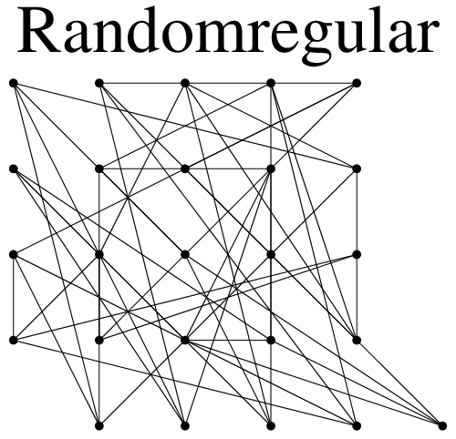
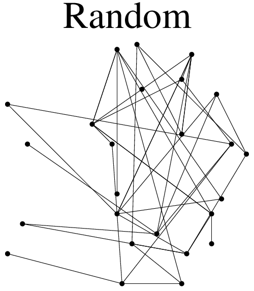
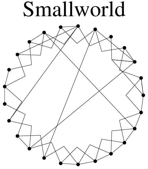
All networks used as an underlying topology for such a game should fulfill some common properties. They should be connected, so that we do not have some parts of the population not being linked to the rest of the population. Here, we always consider undirected and unweighted (binary) graphs. To avoid self-interactions of the agents, self-loops should be excluded. A schematic illustration of the network types used in this paper is shown in Fig. 1.
IV.1 Regular lattice
The first step of complexity of placing vertices spatially – beyond the linear chain – is a regular square (or rectangular) lattice. Typically, each node is connected with or nearest neighbors. To eliminate boundary effects, we use periodic boundary conditions. This is a very simple, but in many cases not realistic model, so we have analyzed some other specific types of models that will be presented in the following subsections. For a better comparability with the regular square lattice with natural connectivity of or , we have restricted ourselves to graphs with an average vertex degree of and .
IV.2 Erdős-Renyi random graph
The most frequently used model of real, not lattice-like graphs in the past decades was the Erdős-Renyi (ER) random graph [37]. Here one starts with a graph with nodes and connects each pair of nodes with probability . In this model the probability of finding a node with degree follows a Poisson distribution
| (11) |
where
| (12) |
The graphs we have investigated are constrained in two ways. On the one hand, they must be connected, what means that there is at least one possibly path from each node to any other so that we don’t have two or more groups of not interrelated agents. On the other hand, we restrict ourselves to networks with a mean vertex
degree of or for better comparability with the regular lattice. Because we will need only connected graphs with a certain mean
degree ,
and because we would find these networks only with some
probability even by adjusting with respect to the number of nodes, we have used the following
algorithm:
- 1.
Start with a graph G with vertices and no edges.
- 2.
Link randomly chosen vertex pairs if they are not already linked until the total number of edges equals . Now the mean vertex degree will equal .
- 3.
If the graph is connected, accept it, otherwise return to step (1).
IV.3 Random regular graph
A compromise between the random graph and the regular lattice is the random regular graph with the same
degree for all vertices but a much shorter average shortest path length than in a lattice. For generating the random regular graphs we have used an algorithm proposed by Steger and Wormald [38]. This algorithm ensures to give connected random graphs with equal
degree for all vertices:
- 1.
Start with a graph G with nodes and no edges.
- 2.
Repeat the following until the set S is empty: Let S be the set of vertex pairs of G that are not connected by an edge yet with both having at most degree . Then choose a specific pair out of S with probability proportional to , where and are the degrees of and in the graph generated up to now. Add the edge to G. Delete the pair from S.
- 3.
If G is -regular (that means connected and of the same degree for all vertices), accept it, otherwise return to step (1).
The last step with the return statement is necessary because unfortunately the algorithm does not exclude the possibility of receiving disaggregated graphs (which occurs rarely) or that the last connection possibilities are only self-loops.
IV.4 Barabási-Albert scalefree network
Many real networks, primarily huge ones, are described by the ER-model in an insufficient way. In many of these networks, for instance the internet [39], the WWW [40, 41], the network of power nodes in the west of the United States [42], the network of scientific collaborations [43], or the metabolic network of yeast [44] one observes a degree distribution that (approximately) follows a power law,
| (13) |
Barabási and Albert [45] have proposed the following algorithm of modelling complex real networks:
- 1.
Start with a small number vertices that are all connected to each other.
- 2.
Add another node and link it to an already present vertex with probability proportional to the degree of this vertex. Add further links in the same fashion until the new vertex has a degree .
- 3.
Repeat step (2) (until you have reached some value of you want).
In contrast to the ER-model for random graphs or the likewise frequently used Watts-Strogatz-Modell ([42], see next subsection) this model incorporates two main aspects of real networks, growth and preferential attachment. Namely, most real networks do not have a fixed size but grow like the WWW [40, 41]. The WWW is also an example for the preferential attachment: When creating a new website, one will typically try to link it to well known and popular sites to gain more attention for ones own site. Because of that, the Barabási-Albert network has a high density of so-called hubs. These are vertices that are connected with many other nodes with relatively small vertex degree.
IV.5 Small-World-Network after Watts and Strogatz
Another frequently used network model is the Small-World network. The existence of long range connections with simultaneous appearance of a high local cluster coefficient is a phenomenon often obtained in real networks [46].). The notion integrates some slightly different types of networks. Here we have used the original model of Watts and Strogatz [42]. In their model one starts with a circle of nodes. All of them are connected with nearest neighbors ( in the one direction and in the other). Afterwards, one starts with rewiring the links, beginning with an arbitrary vertex on the circle. With a certain probability , is disconnected from its nearest neighbor in clockwise direction and is connected to a randomly chosen vertex that is not already linked to . In this way one goes on in clockwise direction until all links to nearest neighbors have been checked for rewiring. Then one goes on with the second nearest neighbor, and so on, until all links have been checked for rewiring.
For one achieves obviously some kind of regular lattice (that is structured in a different way that the one we have used). In contrast to that, for one achieves a graph equivalent to the ER-random graph. But for intermediate values of one gets networks with high local cluster coefficients like a regular graph (or lattice), but also a small average shortest path length like a random graph [47]. For the sake of clarity, we have used in all cases.
IV.6 Network with Gaussian degree distribution
As a sixth type of networks, we have used a graph with a Gaussian degree distribution. This type is a compromise between the ER-random graph and the random regular graph. To generate these networks we have modified the algorithm used for the random regular graph by making the designated vertex degree dependent of , . For these we have used a Gaussian distribution with a standard deviation of , where is the designated average vertex degree. By this choice of the standard deviation it is ensured that almost all designated degrees are positive. We have ignored the few occurring non-positive (negative or ) degrees by choosing a new designated degree in the case of such a choice.
IV.7 Uncorrelated scalefree graph
To analyze possible effects of the vertex degree distribution in scalefree graphs after Barabási and Albert on the dynamics of our games, we have investigated the dynamics on uncorrelated scalefree graphs as well. For the construction of such networks we have used the algorithm described in the preceding subsection (IV.6) with a power law degree distribution identical with the distribution of vertex degrees of the Barabási-Albert scalefree graph instead of a Gaussian distribution. To avoid confusion, we will refer to this graph short as uncorrelated. If we refer to scalefree graphs (without mentioning anything about the correlation) we always consider the Barabási-Albert network.
V Mean extinction times
We have carried out extensive simulations to obtain the mean time until one of the three strategies has gone extinct when starting with each of the strategies having the same frequency (this requires that is an integer multiple of three). After the first strategy has vanished, the game lacks its cyclic dominance, and we return to the two strategy case which is well known and will end up in a much shorter time in a single-strategy steady-state because one of the two remaining strategies definitely dominates the second. Note that we measure time in units of single update steps instead of Monte Carlo steps, where on average each agent has been updated in one time step, so there is a factor of between these two time scales.
V.1 Mean extinction time in well mixed populations
First, let us consider the case of well mixed populations for comparison, which is identical to the case of fully connected graphs (that means each vertex is directly linked to any of the others). We have to distinguish between two cases: the Moran and the local update process on the one hand, and the SPD-process on the other hand.
V.1.1 Moran and local update process in mixed populations
In well-mixed populations, the Moran and local update process have been shown in [13] to have the adjusted replicator equation [48] and the standard replicator equation [3] as limits as goes to infinity. They both have a neutrally stable (for the zero-sum RPS) fixed point in the state space of strategy densities at . For any other point inside of the simplex, both replicator equations predict neutrally stable oscillations around this fixed point, but in the case of finite populations the population can run out of the fixed point and the orbits around it because of stochastical fluctuations, and end up on the edge of the simplex which is the boundary of the state space. A point on the edge of this simplex corresponds to the extinction of at least one of the three strategies (there are three points on the boundary corresponding to the survival of only one strategy). So we expect the MET of this system to tend to infinity as . But at this point there are still two open questions: What is the exact scaling dependence of the MET on ? And how does the selection strength influence this dependence?
Our simulations give clear and short answers for both questions: In the zero-sum RPS game, the MET is proportional to (in single birth-death update steps, corresponding to Monte Carlo steps), and independent of (both is different in the non zero-sum RPS case). For both processes, Moran and local update process as well, we have found the mean extinction time to scale as [12]
| (14) |
V.1.2 SPD-process in mixed populations
As this process has never been defined for unstructured populations let us use the complete graph as a model for the mixed population for simplicity, so that we do not have the risk of making any alterations to this update rule if re-defining it. Now we find that, when starting with , each node has as many neighbors of the dominating strategy as of the dominated one, namely . Because of the structure of the payoff matrix the fitness is identical to zero for every strategy and node. So the condition that the second chosen vertex has a greater fitness than the first is never fulfilled, and one will never observe a change in the strategy densities. For this reason the MET becomes infinite even in finite populations (at least when starting in the point ; even when starting in some neighboured point in the state space we would only achieve some conditional mean extinction time).
V.2 Moran process on networks


From the results of our simulations (see Fig. 2), there are two immediate main observations: First, for some networks biodiversity is greatly stabilized as the MET increases exponentially with , while for other networks biodiversity is only slightly stabilized or even destabilized. Second, the MET is no longer independent of the selection strength even in the zero-sum RPS case that we have considered here. Stabilizing effects of the underlying structure are more distinct for greater .
Great stabilization of the biodiversity is only observed for networks with a heterogenous degree distribution and strong selection, while for networks with homogenous degree distribution we have no such strong stabilization. In fact, the networks with homogenous degree distribution can even lead to a slight destabilization of biodiversity for strong selection, as the MET grows slower than , as we can see for the random regular graph. Even in the cases of the small world and the Gaussian network, which both have a small heterogeneity in their degree distribution, we have such a destabilization. Only for the square lattice we have a stabilization (although the lattice has a homogenous degree distribution, of course), but the stabilization is much weaker than in case of the random graph or the two scalefree networks. For the stabilization on the lattice, the large average shortest path length might play a role (which is proportional to instead of as for random networks [49]).
For small , there is not a great change in the behaviour of the MET on all networks compared to unstructured populations (Fig. 2).
Also, the correlation strength of the network degrees has only minor effect of the stabilization of biodiversity. The MET for an uncorrelated scalefree graph is, in all cases considered here, somewhat smaller than for the Barabási-Albert scalefree graph, but in comparison to the other effects, mainly the enormous stabilization impact of scalefree networks, this is negligible.
V.3 Local update process on networks


One of our main points of interest was whether the evolutionary process itself influences the MET in the case of a networked population. The corresponding results for the Local Update are shown in Fig. 3. There is no qualitative difference between the results in the Moran process and in the Local Update process. Same as for the Moran process, heterogenous degree distributions cause an enormous stabilization of the biodiversity for strong selection (the MET grows exponentially with ), while homogenous degree distributions do not. The MET is now dependent on the selection strength as well, and for small it is proportional to as in the neutral case. The only difference is that stabilizing effects are not as strong as in the Moran process for the same or even a bit larger .
V.4 SPD-process on networks


The SPD-process behaves completely different, as shown in Fig. 4. We recall that for this update rule the quite general observation that spatial discretization can lead to a stabilization of biodiversity does not hold. Even ignoring this and taking a MET scaling for large like the scaling from Moran process and Local Update as reference, for all studied graphs except the lattice we have a destabilization, and the MET grows slower than with only small differences between the different networks. Only in the lattice case the MET grows exponentially with .
Changing the parameter has minor influence on the properties of the MET than the selection strength in the Moran and the Local Update process. For degree homogenous networks, the MET is even independent of . For networks with a strong heterogeneity in the degree distribution the MET grows with for the same value of .
There is also some influence of the correlation of network degrees. For the uncorrelated scalefree network, the influence of the parameter on the MET is not as great as for the Barabási-Albert network, and the METs for the same , but different and are closer together. But compared to the other effects, this is again negligible.
VI Theoretical approach
VI.1 Moran process
VI.1.1 General case
For a version of the RPS game with constant reaction rates it has already been shown that networks with heterogenous degree distribution effect a stabilization of biodiversity [50]. This corresponds with our simulation results so we have adapted the approach from [50] to underpin the shown behaviour theoretically.
First let us define the probability density of the strategy on all nodes with degree as . Here we again use the notation for an arbitrary strategy, for the strategy dominated by , and for the dominating strategy. Then the probability that a neighbored node of an arbitrary vertex plays strategy reads
| (15) |
Here is the probability of finding a vertex with degree . Dividing by the average vertex degree, , assures the standardization. Further, by the conservation of the total density one of the quantities and of is given so that we can eliminate and using and as variables, or and , respectively
| (16) | |||||
| (17) |
The average payoff of a player of strategy on a node with degree is then given by
| (18) |
We find that the average payoff is independent of the vertex degree so we can drop the index , . With this we can compute the average payoff of neighbours of a vertex
| (19) | |||||
By using instead of we consider that is more likely to have a vertex with a high degree as a neighbour than one with a smaller degree if both are equally frequent. Thus we find the probability for a player with strategy sitting on a node with degree to reproduce as
| (20) |
and the rate with that a player of strategy sitting on a vertex with degree conveys his strategy to a node with degree , which has played strategy before, reads
| (21) | |||||
For ( is the Kronecker symbol) this reduces to
| (22) |
Here we have omitted any -indices because there is only one degree left. The payoffs reduce to and , and one obeys the hopping rates for the Moran process in well mixed populations [11] independent of . This rate describes how likely it is that a player with strategy is replaced by a copy of another player with strategy in a single time step.
Let us now consider a heterogenous degree distribution. In the simplest case, such a distribution consists of only two degrees and with frequencies and , respectively. The replicator equation that we obtain from the master equation in the limit for the changing of the frequency of the strategy on nodes with degree reads (for the methodology see e.g. [51, 13, 52]):
| (23) | |||||
Inserting our special degree distribution, after a longish but straightforward calculation we find
| (24) | |||||
Here is the background fitness. is the mean fitness of all players on vertices with degree , and correspondingly for . Then one can compute the other equations in an analogical way or by cyclically permuting the indices. For each vertex degree, one of the equations of motion needs not to be taken into account by the constraint . For or alternatively this flattens to the well known adjusted replicator equation in the case of well mixed populations, as expected [13, 14]. Likewise, the fixed point of this replicator equation at does not alter, we now just have two densities for every strategy. But now the velocity of the reaction is directly dependent of because it is no longer possible to absorbe the strength of selection by a dynamical rescaling of time, as it is possible for well mixed populations.
But what about the stability of this inner fixed point? Within a linear stability analysis, let us linearize the replicator equation around its fixed point
| (25) |
with and being the Jacobian of the system with . In our case, we find as
| (26) |
To reason about the stability we need to know the signs of the real parts of the eigenvalues of this matrix, but for these eigenvalues we derive quite complicated terms, the signs of which cannot be easily designated (but see Appendix A). The Routh-Hurwitz criterion as an alternative solution does not simplyify the situation considerably.
Approximating an upper bound of the real parts of all eigenvalues, it is possible to compute a region in the parameter space where the inner fixed point is guaranteed to be asymptotically stable, namely, for
| (27) |
For a given value of this determines the ratio of and , or, the other way round, if we want to build up a network with chosen values for and , this inequality tells us what frequencies of both vertex degrees are necessary to stabilize biodiversity. So, for example, if we choose and both vertex degrees should be equally frequent, must be at least to fulfill this inequality. If a higher frequency of is desired, must even be larger.
But as this is just a rough approximation, by inserting numerical values we have found that almost all eigenvalues are , except for the trivial cases , or . So for all values except these mentioned cases, we have found the fixed point to be asymptotically stable. Here, we have found numerically that the real parts of the eigenvalues become more negative as the difference of and grows in absolute size, and both vertex degrees become equally likely to be found in the network. This explains as well why the stabilization of biodiversity is greater in the case of the scalefree graphs than for the ER-random graph, or it is in both cases greater than for the network with a gaussian degree distribution, which has only as small heterogeneity in its degree distribution.
VI.1.2 Small selection limit
As we have seen in the previous section, for small the MET is almost proportional to as in the well mixed case, and depends only marginally on the underlying network structure. We can intuitively understand this as follows: If is small, than every transition probability is , and the corresponding replicator equation in our system reads
| (28) |
for all values of and . Hence, each point of the state space is a neutrally stable fixed point in the limit . Therefore there should be no stabilization impact compared to the well mixed case, as there each point in the simplex belongs to a neutrally stable limit cycle, so in both cases a perturbation is neither expected to decay nor to grow in time.
VI.2 Local update process

Following the same scheme as for the Moran process, one can derive similar results (see Appendix B for details). As in the Moran process, a degree heterogeneity leads to a stabilization of biodiversity, but again the eigenvalues of the Jacobian are too byzantine for catching the signs of the real parts easily.
VI.3 SPD-process
For this update process, we will use a simpler method to achieve a theoretical understanding of some of the numerical results. In the case of both chosen vertices having the same degree, the probability for the node to change its strategy to the strategy of simplifies to
| (29) |
So for the lattice and the random regular graph, where all vertex degrees are the same, any dependence of drops out. Note that in this equation and in this whole subsection, when talking about we consider the not modified payoffs. For one achieves the same term as in the case of degree homogenous networks (eq. 29), independent of the network, while for we find
| (30) |
or
| (31) |
respectively, depending on which of the vertex degrees is greater. If we compare the probabilities for and for by computing the ratio of both, we can analyze the impact of the parameter and the underlying network structure on the MET. We find
| (32) |
or
| (33) |
respectively. If we account for the fact that must hold, then the first fraction is for and for . Hence, if aside from all conditions are the same, for it is more likely that a strategy with a lower payoff reproduces, if ) than for . On the other hand under these conditions for it is less likely that a strategy with a high payoff reproduces, than for . In the second case, the fraction is for and and for all other cases. Hence for it is more likely that a strategy with a high payoff replaces a strategy with a smaller payoff from a node with a smaller vertex degree, than for . And for under this conditions it is as much more likely that a strategy with a smaller payoff reproduces. Taken together, for strategies with a smaller payoff have a bigger chance to reproduce, and they are less likely to be replaced by a strategy with a higher payoff, than for . Hence on degree-heterogenous networks the MET should be greater for than for , as it is confirmed by the simulation results (Fig. 4).
VII Conclusions
Cyclic coevolutionary dynamics manifests an interesting class of dynamical systems that are discussed as models to explain long-term stabilization of coexistence of species or strategies. In this paper we have shown that, for the coevolutionary RPS game on complex networks, there are considerable differences in the mean extinction time (MET) between different networks, and for different processes as well. The simple statement “Spatial discretization stabilizes biodiversity” must be refined in a more sophisticated way. While for example in the Moran and in the local update process degree-heterogenous networks preserve biodiversity (the MET grows exponentially with the number of players), in the SPD-process they do not, and even degree-homogeneous networks may destabilize while the lattice still stabilizes. In summary, we have shown that, for the cyclic evolutionary RPS on networks, there is a striking influence on the mean extinction time characteristics of the spatial structure and the update rule as well.
Appendix A Eigenvalues of the Jacobian in equation (26)
With the help of (e.g.) Mathematica™ one can easily compute the eigenvalues of the Jacobian in equation (26):
| (34) | ||||
| (35) | ||||
| (36) | ||||
| (37) | ||||
with the abbreviations
| (38) | |||||
| (39) | |||||
The real parts of this eigenvalues are then given by
| (40) | |||||
| (41) | |||||
| (42) | |||||
| (43) | |||||
Here, is the argument of the complex number . The sum of the first four terms negative in each case because and for this reason . The problem is the last summand, but it is possible to make a rough approximation of where all real parts are negative. As and , all real parts are smaller than
| (44) |
Inserting and and assuming without loss of generality, one can approximate the fourth root in the last term by
| (45) | |||||
As the have checked numerically, the remaining root divided by for (which is necessary to have mathematically meaningful probabilities between and ), so
| (46) |
and therefore all real parts are negative if
| (47) |
or noted in a simplified way and remembering the assumption at the beginning of this approximation,
| (48) |
.
Appendix B Theoretical approach: local update process on networks
Similar as in the Moran process, in the local update process on networks the rate with which vertices with degree and strategy carry this strategy over to nodes with degree and strategy is given by
| (49) |
which does not vary from the results in well mixed populations in the case of homogenous degree distribution. The replicator equation for the model system of a heterogenous degree distribution with only two vertex degrees reads
| (50) | |||||
with . The other equations are obtained analogously. Here again the position of the fixed point is not changed compared to the well mixed case. But again it is no longer possible to absorb the selection strength by a rescaling of time.
A linear stability analysis leads to the matrix
| (51) |
The eigenvalues of this matrix are again given by
| (52) | ||||
| (53) | ||||
| (54) | ||||
| (55) | ||||
with the abbreviations
| (56) | |||||
| (57) | |||||
The real parts of this eigenvalues are given by
| (58) | |||||
| (59) | |||||
| (60) | |||||
| (61) | |||||
which is very similar to the corresponding result in the Moran process (it varies only slightly in and ). Searching for an upper bound for the real parts of the eigenvalues, we even derive the same inequality as for the Moran process
| (62) |
References
- [1] Gintis, H., Game Theory Evolving, (Princeton Univ. Press, Princeton, 2000)
- [2] M.A. Nowak, Evolutionary Dynamics, Belknap Press (2006)
- [3] Hofbauer, J., and Sigmund, K., Evolution and the Theory of Games, Cambridge University Press, Cambridge, England, (1998)
- [4] Szabó, G., and Fáth, G., Evolutionary games on graphs, Physics Reports, 446, 97-216 (2007)
- [5] Roca C.P., Cuesta J.A., Sanchez A., Evolutionary game theory: Theoretical and spatial effects beyond replicator dynamics, Physics of Life Reviews 6 (4), 208-249 (2009)
- [6] Hauert, C., De Monte, S., Hofbauer, J., and Sigmund, K., Volunteering as red queen mechanism for cooperation in public goods games, Science 296, 1129 (2002)
- [7] Czárán, T.L., Hoekstra, R.F., and Pagie, L., Chemical warfare between microbes promotes biodiversity, Proceedings of the National Academy of Sciences, USA, 99, 786-790 (2002)
- [8] Kerr, B., Riley, M.A., Feldman, M.W., and Bohannan, B.J.M., Local dispersal promotes biodiversity in a real-life game of rock - paper - scissors, Nature 418, 171-174 (2002)
- [9] Sinervo, B., and Lively, C., The rock-paper-scissors game and the evolution of alternative male strategies, Nature 380, 240, (1996)
- [10] Durrett, R., and Levin, S., Allelopathy in spatially distributed populations, Journal of Theoretical Biology 185, 165-174 (1997)
- [11] Claussen, J.C., Traulsen, A., Cyclic dominance and biodiversity in well mixed populations, Physical Review Letters 100, 058104 (2008)
- [12] Schütt, M., and Claussen, J.C., Mean extinction times in cyclic coevolutionary rock- paper-scissors game: Numerical and analytical results, (in preparation)
- [13] Traulsen, A., Claussen, J.C., and Hauert, C., Coevolutionary dynamics: from finite to infinite populations, Physical Review Letters 95, 238701 (2005)
- [14] Traulsen, A., Claussen, J.C., and Hauert, C., Coevolutionary dynamics in large, but finite populations, Physical Review E 74, 011901 (2006)
- [15] C. Hauert and M. Doebeli, Spatial structure often inhibits the evolution of cooperation in the snowdrift game, Nature (London) 428, 643 (2004)
- [16] K. Lindgren and M. Nordahl, CEvolutionary dynamics of spatial games, Physica D 75, 292 (1994)
- [17] A. V. M. Herz, Collective phenomena in spatially extended evolutionary games, J. Theor. Biol. 169, 65 (1994)
- [18] Axelrod, R., and Hamilton, W.D., The evolution of cooperation, Science 211, 1390 (1981)
- [19] Nowak, M.A., and May, R.M., Evolutionary games and spatial chaos, Nature 359, 826-829, (1992)
- [20] Nowak, M.A., and May, R.M., The spatial dilemmas of evolution, Int. J. Bifurcat. Chaos 3, 35-78 (1993)
- [21] Roca, C.P., Cuesta, J.A., and Sánchez, A., Promotion of cooperation on networks? The myopic best response case, arXiv:0901.0355v1, (2009)
- [22] Szolnoki, A., Perc, M., and Danku, Z., Towards effective Payoffs in the prisoner’s dilemma on scalefree networks, Physica A 387, 2075-2082 (2007)
- [23] Traulsen, A., and Claussen, J.C., Similarity based cooperation and spatial segregation, Physical Review Letters E 70, 046128 (2004)
- [24] G. Szabó and C. Tőke, Evolutionary prisoner’s dilemma game on a square lattice, Phys. Rev. E 58, 69 (1998)
- [25] G. Szabó and C. Hauert, Phase transitions and volunteering in spatial public goods games, Phys. Rev. Lett. 89, 118101 (2002)
- [26] Thomas Butler and Nigel Goldenfeld, Robust ecological pattern formation induced by demographic noise, Phys. Rev. E 80, 030902(R) (2009)
- [27] Buss, L.W., Competitive intransitivity and size-frequency distributions of interacting populations, Proceedings of the National Academy of Sciences, USA, 77, 5355 (1980)
- [28] Gilg, O., Hanski, I., and Sittler, B., Cyclic dynamics in a simple vertebrate predator-prey community, Science 302, 866 (2003)
- [29] Maynard Smith, J., The games lizards play, Nature 380, 198 (1996)
- [30] Moran, P.A.P., The statistical processes of evolutionary theory, Clarendon Press (1962)
- [31] Nowak, M.A., Sasaki, A., Taylor, C., and Fudenberg, D., Emergence of cooperation and evolutionary stability in finite populations, Nature (London) 428, 646 (2004)
- [32] C. Hauert and G. Szabó, Game theory and physics, Am. J. Phys. 73, 405 (2005)
- [33] D. Helbing, Physica A 181, 29 (1992)
- [34] D. Helbing, Physica A 193, 241 (1993)
- [35] L. E. Blume, The statistical mechanics of strategic interaction, Games and Economic Behavior 5, 387 (1993)
- [36] Claussen, J.C., Drift reversal in asymmetric coevolutionary conflicts: Influence of microscopic processes and population size, The European Physical Journal B 60, 391-399(2007)
- [37] Erdős, P., and Rényi, A., On the Evolution of Random Graphs, Publ. Math. Inst. Hung. Acad. Sci. 5, 17 (1960)
- [38] Steger, A., and Wormald, N.C., Generating random regular graphs quickly, Combinatorics, Probability and Computing 8, 377-396, (Cambridge University Press, England, 1999)
- [39] M. Faloutsos, P. Faloutsos, and C. Faloutsos, On Power-Law Relationships of the Internet Topology, p. 251-262 in: Proc. Applications, technologies, architectures, and protocols for computer communication, Cambridge, MA, (1999)
- [40] Lawrence, S., and Giles, C.L., Searching the world wide web, Science 280, 98 (1998)
- [41] Lawrence, S., and Giles, C.L., Accessibility of information on the web, Nature 400, 107 (1999)
- [42] Watts, D.J., and Strogatz, S.H., Collective dynamics of small-world networks, Nature 393, 440 (1998)
- [43] Redner, S., How popular is your paper? An empirical study of the citation distribution, Eur. Phys. J. B 4, 131 (1998)
- [44] Jeong,H., Tombor, B., Albert, R., Oltvai, Z.N., and Barabási, A.-L., Nature 407, 651-654, (2000)
- [45] Barabási, A.-L., and Albert, R., Emergence of scaling in random networks, Science 286, 509 (1999)
- [46] Watts, D.J., and Strogatz, S.H., Small world, Nature (1998)
- [47] Albert, R., and Barabási, A.-L., Statistical mechanics of complex networks, Rev. Mod. Phys 74, 47 (2002)
- [48] Maynard Smith, J., Evolution and the Theory of Games, (Cambridge University Press, Cambridge, England, 1982)
- [49] Newman, M.E.J., Strogatz, S.H., and Watts, D.J., Random graphs with arbitrary degree distributions and their applications, Physical Review E 64, 026118 (2001)
- [50] Masuda, N., and Konno, N., Network-induced species diversity in populations with cyclic competition, Physical Review E 74, 066102, (2006)
- [51] N. van Kampen, Stochastic processes in physics and chemistry. North Holland, Amsterdam (1981)
- [52] McKane, A. J., and Newman, T. J., Predator-Prey Cycles from Resonant Amplification of Demographic Stochasticity, Phys. Rev. Lett. 94, 218102 (2005)
- [53] Julia Poncela, Jesús Gómez-Gardeñes, Arne Traulsen, and Yamir Moreno, Evolutionary game dynamics in a growing structured population, New J. Phys. 11 083031 (2009)