Quartet of spin-3/2 baryons in chiral multiplet with mirror assignment
We study the possible existence of chiral partners in the spin- sector of the baryon spectrum. We consider a quartet scheme where four spin-3/2 baryons, , , and , group into higher-dimensional chiral multiplets with a mirror assignment. With an effective Lagrangian, we derive constraints imposed by chiral symmetry together with the mirror assignment on the masses and coupling constants of the quartet. Using the effective Lagrangian, we try to find a set of baryons suitable for the chiral quartet. It turns out that two cases reasonably agree with the mass pattern of the quartet: (, , , ) and (, , , ).
1 Introduction
Chiral symmetry and its spontaneous breaking characterize the QCD vacuum, and is a key to understanding the strong interactions. Due to the spontaneous breaking of chiral symmetry (SBCS), the hadron spectrum is classified in terms of the residual symmetry , while the role of in the hadron spectrum is unclear. Nevertheless, one expects that there exists a set of hadrons reflecting a nature of the original symmetry, which is referred to as chiral partners. Such examples are well-known for mesons, e.g. and [1, 2, 3], while not well established for baryons. As discussed in the meson’s case, finding chiral partners provides us with the understanding of the role of chiral symmetry in the hadron spectrum, and also a clue to study the restoration of chiral symmetry. Recently, the multiplet nature of the chiral group draws a renewed attention from an interest in the effective chiral restoration [4, 5, 6], which was suggested to be the cause of the observed parity doubling in high-energy region of the spectrum [7].
In the present work, we address the issue of the multiplet nature of the baryon’s chiral partners. We denote a chiral multiplet by , where is an isospin for . All the members of one chiral multiplet have a fixed spin. The correspondence of the charge algebra between and leads to a relation . This implies that a chiral multiplet can contain various isospin states. In the presence of the SBCS, the mixing of different chiral representations happens, and a hadron with an isospin can be described as a superposition of various chiral representations containing . We are here concerned with the case that a set of hadrons group into one or a few representations even in the presence of the SBCS, or the case where the configuration mixing is small.
In order to find chiral partners, we need to understand the multiplet nature of the chiral group, such as the pattern of the spectrum and coupling constants of the multiplet. Because general relations for masses and axial charges that can be applied to arbitrary chiral representations are not established so far, the properties of the chiral partners are usually studied with focusing on a particular chiral representation. In the meson’s case, the properties of chiral partners have been investigated by using e.g. the NJL model [8, 9] and Weinberg sum rules [10]. The NJL model was applied to the nucleon [11, 12, 13, 14, 15] and [16] by solving the Faddeev equation. We applied the NJL model with diquarks to the nucleon [17, 18, 19] and the Roper resonance [20], using an auxiliary field method. However, when we apply such microscopic approaches to a baryon with a mass larger than sum of the masses of the internal degrees of freedom, we encounter the difficulty of the confinement. Due to this difficulty, effective Lagrangian approaches that contain hadrons as degrees of freedom are often employed for the study of baryon’s chiral partners [21, 22, 23, 24, 25, 26, 27, 28].
In recent papers, we have developed a systematic method to construct an effective Lagrangian including higher-dimensional representations [29, 30, 31, 32, 33], which we refer to as a projection method. This method is inspired by an NJL model for mesons, and partly extend it to baryons. In Ref. [29], we classified baryon fields consisting of three quarks in terms of chiral multiplets. The Pauli principle implemented by the Fierz transformation plays a crucial role in the classification. The projection method is performed as follows. First we find a chiral invariant operator involving direct products of the quark and diquark fields. This can be achieved by using an analogy between and diquarks in chiral transformation property. Then, we project the direct products of the quark and diquark fields onto irreducible parts with the use of the Fierz identities. After the projection, three-quark fields are replaced by baryon fields. Thus we can systematically construct chiral invariant Lagrangians including higher-dimensional chiral representations, avoiding problems caused by the lack of the confinement. Although such simple effective Lagrangians have limited validity, they are useful for the present purpose to derive the pattern of the masses and coupling constants of the chiral multiplet.
In Ref. [30], we have applied the projection method to a quartet scheme (QS). The QS was first proposed by Jido et. al. [34]. They used two kinds of and considered so-called mirror assignment [22, 23, 25], where four types of baryons, two with and the other two with , are included in the multiplet. They applied the QS to and and studied the masses and intra-coupling constants of the quartet. They did not consider Dirac structure of the Lagrangian explicitly. Owing to the projection method, we took intro account the Dirac structure in the QS Lagrangian which enables us to include transition terms between and , e.g. and . With the QS Lagrangian, we have derived several constraints on the masses and coupling constants, which characterize the multiplet nature of the quartet.
In the present work, we develop the previous study to find a set of baryons suitable for the chiral quartet of spin- baryons. Considering , the quartet consists of , , , and . Among various candidates for this set, we adopted a particular assignment in Ref. [30]: , , , . It is an important question if there is other assignment suitable for the quartet. One interesting assignment is a set (, , , ). Glozman mentioned the possibility that the approximate degeneracy of these four baryons is a consequence of the effective chiral restoration [6]. If this is the case, there are two possibilities. The first one is that the four baryons form the chiral quartet. The second one is that two s belong to and two belong to . We can study the first case using the QS Lagrangian.
In order to take into account interactions in the QS, it is necessary to determine the nucleon’s chiral representation. In standard linear models of Gell-Mann-Levy type [21] the nucleon belongs to . In the mirror models [22, 23, 24, 25, 26, 27], the nucleon is a mixture of two kinds of . The mixing of and was studied in an algebraic approach [35, 36, 37] and field theoretical approaches [32, 33]. In non-relativistic quark models the nucleon wave-functions also correspond to the mixing of and . In the present study, we assume the nucleon to be saturated with the fundamental representation due to the following reasons. The linear models qualitatively describe the chiral properties of the nucleon. For instance, the linear models describe in qualitative agreement with . Secondly, the nucleon belongs to , if the nucleon operator has spatially symmetric property [29].
This paper is organized as follows. In section 2, we define the baryon fields and derive their transformation properties. In section 3, we construct the Lagrangian, such as mass terms and interactions with the use of the projection technique. Here denotes the member of the chiral quartet. Although the QS Lagrangian is not new, we generalize the formulation given in the previous study in a assignment-free manner in order make it feasible to test various assignment. With the Lagrangian, we derive several constraints on the properties of the quartet. Because the projection method is complicated, we show an alternative derivation of some of the present results, using chiral algebra in Appendix B. Numerical results are shown in section 4. Considering the masses, we find two suitable assignments (, , , ) and (, , , ). We discuss the properties of the quartet for these cases together with the assignment (, , , ). The final section is devoted to a summary.
2 Chiral Properties of Baryon Fields
In this section, we consider baryon fields consisting of three quarks, which serves as a preparation for the projection method. Baryon fields consisting of three quarks in a local form are generally described as
| (1) |
where is an iso-doublet quark field at location , the superscript represents the transpose and the indices and represent the color. The antisymmetric tensor in color space ensures the baryons being color singlets. From now on, we shall omit the color indices and space-time coordinates. describe Dirac and isospin matrices. With a suitable choice of , a baryon field is defined so that it forms an irreducible representation of the Lorentz and isospin groups.
Concerning , there are three possible baryon fields with ;
| (2a) | ||||
| (2b) | ||||
| (2c) | ||||
| and two with ; | ||||
| (2d) | ||||
| (2e) | ||||
where is a transposed quark field. Here we employ an isospurion formalism [38, 39] for an isospin- projection operator , which is given by Similarly, is a local spin- projection operator defined by . In the present work, we consider only on-shell spin- states. In order to consider off-shell spin- baryons, we need to employ the non-local projector instead of the local one [40, 41, 42, 43].
Note that the baryon fields Eqs. (2) are not independent [44, 45, 46]. In addition, they belong to reducible chiral representations, which leads to unphysical mixings of different chiral representations [29]. The cause of the unphysical chiral mixings is the fact that Eqs. (2) are not totally anti-symmetric; they are anti-symmetric only for the interchange between the first and second quarks. Considering the Fierz transformation as the anti-symmetrization of the second and third quarks, we obtain the totally-antisymmetric baryon fields
| (3a) | ||||
| (3b) | ||||
These totally-antisymmetric combinations belong to the irreducible chiral multiplet [29]. The derivation of Eq. (3) is shown in Appendix A.
With the baryon fields consisting of the quark fields, it is straightforward but tedious task to derive their transformations by using that of the quark field : with being the infinitesimal parameters for . We obtain
| (4a) | ||||
| (4b) | ||||
which contain off-diagonal terms and as well as the diagonal ones. They restrict possible chiral invariant terms, similar to the case of in the linear sigma model.
For later convenience, we define diquark fields contained in the spin- baryon fields: a Lorentz vector isoscalar diquark (), a Lorentz axial-vector isovector diquark ()
| (5a) | ||||
| (5b) | ||||
It is easy to check that and correspond to and mesons in chiral transformation properties, which is a key of the projection method.
We introduce the other set of : , where they have the same spin and isospin as the original ones , but the opposite transformation properties in sign, i.e.,
| (6a) | ||||
| (6b) | ||||
This property is referred to as the mirror assignment [25], and we refer to as naive, and to as mirror. There is a correspondence of the chiral transformation properties between the naive and mirror sets,
| (7) |
where the indices and denote the left- and right-handed projection with the projection operator . The right-handed parts of and have the same chiral transformation properties as the left-handed parts of and , and vice versa.
Note that we defined and by their transformation properties Eqs. (6). It is useful to define the baryon fields for and . It is impossible to describe them in terms of local three-quark fields. Since baryons are composite particles, there are generally various possible expressions for and . For example, we can describe them by using baryon operators having a derivative,
| (8a) | ||||
| (8b) | ||||
| (8c) | ||||
where denotes a covariant derivative. The mirror fields and are obtained by the same equations as Eqs. (3) with substitution of the primed fields for the original fields . Although they would not be a unique possibility for the microscopic description of the mirror fields, Eqs. (8) are enough for the present purpose to construct the chiral invariant Lagrangian.
3 Lagrangian
Now, we proceed to the construction of the Lagrangian. It is straightforward to show the chiral invariance of the kinetic terms: In order to find interaction terms for higher-dimensional chiral multiplets, it is useful to employ the projection method.
3.1 Mass terms and terms
The vector and axial-vector diquarks belong to the chiral multiplet , and is a chiral scalar. The Gell-Mann-Levy type interaction for the quark is also a chiral scalar, where . Obviously, the following combination of these two terms is also a chiral scalar,
| (9) |
This term contains the direct products of the quark and diquark : and . They are decomposed into the irreducible parts as
Substituting Eqs. (10) into the chiral invariant term (9), we obtain
| (11) |
where we omit terms, which contain the Gell-Mann-Levy type interaction with local nucleon operators and . The transition terms between and fields vanish due to . The Lagrangian (11) describes several kinds of the interactions; the first three terms describe the diagonal interactions for and with and , and the fourth term describes a transition between and with , where a coupling vanishes due to .
The diagonal interactions with generate the masses of and in the presence of the SBCS [MeV]. We obtain a mass relation . If we assign with , which is the lowest lying state for , its partner has the mass of MeV. We do not find a baryon suitable for this mass relation in the experimental data [47].
There are several directions to solve this mass problem: the inclusion of higher order terms in the Lagrangian and of higher-order diagrams, the extension of the chiral basis such as and of the mirror assignment. It was shown [34] that the inclusion of the mirror assignment reasonably reproduces the masses and some properties of observed baryons. Using Eq. (7), we find a chiral invariant interaction term
| (12) |
which is almost the same as Eq. (11). The difference appears in the signs of the terms accompanying , which is a feature of the mirror assignment [25].
Considering Eqs. (4), (6) and (7), is chiral invariant, which leads to the following term,
| (13) |
which describes off-diagonal mass terms between and and between and . The parameter describes a chiral scalar, so called mirror mass [25].
The mass terms included in are rewritten in the following matrix forms
Because of the off-diagonal terms in these mass matrices, physical states and their masses are obtained through the diagonalization of the mass matrices. Note that the mass eigen-values can take both positive and negative values. A state with a negative eigen-value can be transformed into a state with a positive mass, but has opposite parity to the original state. It is carried out by multiplying a state having negative mass by [25]. In the present paper, we consider the case that two states form a pair of positive and negative parity states both in and sectors.
For the part in Eq. (3.1), we obtain the mass eigen-values of two states
| (23) |
and the eigen-states
| (24a) | ||||
| (24b) | ||||
| (24c) | ||||
Here we define and as positive and negative parity states, respectively, where the indices denote the parity. Hence and are identified with and , respectively. Note that in Eq. (24b) appears due to the parity redefinition. Similarly, for part, we obtain the mass eigen-values
| (25) |
and the eigen-states
| (26a) | ||||
| (26b) | ||||
| (26c) | ||||
and are identified with and , respectively. Again, in Eq. (26b) appears due to the parity redefinition. The four masses and are given by the three parameters , and , which offers constraints on the four masses [34],
| (27a) | ||||
| (27b) | ||||
The inequality in the first line of Eq. (27) is controlled by . Thus, the mass splittings and average masses are determined by chiral symmetry and the mirror mass .
It is worthwhile considering the correspondence between the basis states and the physical states. Obviously, the mixing angles vanish in the absence of the mirror mass; for . In this limit, the naive and mirror sectors decouple, and the physical states correspond to the basis states : and . It should be noted that the decoupling of the two sectors does not violate chiral invariance. Contrarily, the two sectors are maximally mixed in the dominant case : .
The Lagrangians (11) and (12) contain the one-pion interaction terms between the spin- baryons () as well as the mass terms. Having the four spin- baryons, there are ten coupling constants ; four diagonal and six off-diagonal terms. All the ten coupling constants are functions of and , which are determined by the masses. It is straightforward to derive the coupling constants, from Eqs. (11) and (12). For part, we obtain
| which are defined by Here and denote parity, i.e., or , and for and for . For part, we obtain | ||||
| which are defined by . For - transition terms, | ||||
| which are defined by . | ||||
In order to understand the features of , it is useful to consider the axial-charges, which are obtained by the Noether theorem
In the limit (), the absolute values of the parity-non-changing interactions reach the maximum values: , and , while the parity-changing terms vanish . The mixing angles larger, as becomes larger. Since the naive and mirror sectors have the opposite axial-charges, the mixing of the two sectors suppresses the parity-non-changing interactions and enhance the parity-changing interactions. In the -dominance, the parity-non-changing interactions vanish , while the parity-changing terms reach the maximum values , and . Of course, have the same features as the axial-charges due to the Goldberger-Treiman (GT) relations:
3.2 Interaction with the nucleon
Next, we construct the interactions between the nucleon and the chiral quartet. As we have discussed in the introduction, we assume that the nucleon belongs to . With the nucleon’s chiral multiplet, we can classify the products of the chiral properties of :
where we omit four-meson terms and . In the derivation of Eq. (3.2), it is important to take into account the chirality conservation. This classification implies that chiral invariant interactions between and accompany two-meson fields, while those between and accompany one-meson fields.
We find two chiral scalars and . Multiplying them, we find two chiral invariant terms; , . Using Eqs. (10), we obtain the chiral invariant interaction terms between and
| (47a) | |||||
| (47b) | |||||
| where the dimensional parameter [mass] is introduced to keep the coupling constants and dimensionless. We also introduce shorthand notations for mesonic operators | |||||
| (47c) | |||||
| (47d) | |||||
| (47e) | |||||
| (47f) | |||||
One may think it possible to construct similar interaction terms for the mirror fields by the replacement Eq. (7). However, such terms are forbidden by chirality conservation, as is shown in Eq. (3.2) 11 1 It can be shown explicitly. For example, the first term in Eq. (47a) is rewritten in terms of left- and right-handed parts of the fields as Replacing , , which vanishes due to .. The mirror fields have one-meson interactions with the nucleon. It can be constructed by using the chiral invariant operators and . We obtain
| (48a) | |||||
| where and are also mesonic operators, | |||||
| (48b) | |||||
| (48c) | |||||
In the mass basis, is rewritten as
| (49) |
which contains several kinds of the interaction terms, , , and . Among them, we consider and interaction terms in order for the comparison with experiments. The interactions of the chiral quartet are given by
| (50a) | ||||
| where the coupling constants and are given by | ||||
| (50b) | ||||
| (50c) | ||||
| (50d) | ||||
| (50e) | ||||
Four are expressed in terms of three parameters and , which leads to one identity
| (51) |
Here it must be noted that the derivation of the interactions is based on the assumption of the nucleon’s chiral multiplet. If the nucleon together with the negative parity resonance group into with the mirror assignment, we can include three additional interactions, which spoils the constraint Eq. (51). Another possibility is that the nucleon contains as well as . In this case, we can include one additional interaction that have similar form to Eq. (11). With the new term, Eq. (51) becomes loose constraint and gives the ordering of the coupling constants. So, Eq. (51) is one of the most strict constraint. The point is that it is possible to improve this result without changing the masses and interactions of the quartet.
We obtain two-pion interaction terms
| (52) | ||||
| (53) |
with
where they are classified into three types: the symmetric (), anti-symmetric and symmetric type . They corresponds to an isoscalar (), isovector and isotensor . Since the two-pion coupling constants contain only and , their strengths are determined by the coupling constants through and . Furthermore, are proportional to either or , which provides a selection rule; either isoscalar or isovector interaction is suppressed each for , and either the isovector or isotensor interaction is suppressed each for .
Using the Lagrangian, we have derived several constraints on the properties of the chiral quartet. We concentrate on the construction of the lowest-order terms and the derivation of the chiral constraints at tree level. In general, it is possible to insert chiral invariant operators such as into the chiral Lagrangians we derived. However, those terms does not change the above constraints and can be absorbed into the parameters. Regarding the interactions, it is possible to include additional interaction term with a derivative [25]. The constraint for the interactions rely on the assumption of the saturation of in the nucleon. The inclusion of component in the nucleon causes one additional chiral invariant interaction term similar to Eq. (11). In this case, four are given by four parameters. It must be noted that the inclusion of for the nucleon does not affect the multiplet nature of the quartet.
4 Results
| Observed states | |
|---|---|
| , , | |
| , | |
| , , | |
| , |
| States | [MeV] | [MeV] | [GeV |
|---|---|---|---|
| 1231-1233 (1232) | 116-120 (118) | 15.7-16.0 (15.8) | |
| 1550-1700 (1600) | 25.0-113 (68.8) | 2.37-5.04 (3.70) | |
| 1670-1750 (1700) | 20.0-80.0 (50.0) | 6.34-12.7 (9.51) | |
| 1950-2030 (1990) | 17.0-62.4 (39.7) | 3.23-6.20 (4.72) | |
| 1515-1525 (1520) | 55.0-81.3 (68.1) | 7.64-9.30 (8.46) | |
| 1700-1750 (1720) | 15.0-60.0 (37.5) | 1.72-3.44 (2.58) |
| Case (3-1) | ||||
|---|---|---|---|---|
| States | [MeV] | [MeV] | [GeV | Reference |
| 1900-1970 (1920) | 7.50-60.0 (33.8) | 0.825-2.33(1.58) | PDG average [47] | |
| 1950-2030 (1990) | 17.0-62.4 (39.7) | 3.23-6.20(4.72) | Horn et. al. [48] | |
| 1945-1947 (1946) | 85.2-121 (103) | 4.63-5.23(5.08) | Penner et. al. [49] | |
| 1855-1975 (1915) | 2.80-19.8 (11.3) | 0.574-1.53(1.05) | Nikonov et. al. [50] | |
| Case (3-2) | ||||
| States | [MeV] | [MeV] | [GeV | Reference |
| 1900-1970 (1920) | 7.50-60.0 (33.8) | 0.825-2.33 (1.58) | PDG average [47] | |
| 1947-2167 (2057) | 8.40-234 (121) | 2.04-10.8 (6.40) | Manley et. al. [51] | |
| 1749-1859 (1804) | 53.0-165 (109) | 4.45-7.84 (6.15) | Manley et. al. [51] | |
| 1855-1975 (1915) | 2.8.0-19.8 (11.3) | 0.574-1.53 (1.05) | Nikonov et. al. [50] | |
In this section, we proceed to numerical discussions and look for a set of baryons suitable for the QS. Possible candidates for the members of the quartet are shown in Table 1. There are six parameters in our model: , , and . The dimensional parameter does not play any role in the present study, then we do not need to determine it. Since the masses and are the functions of , and , we can determine them by minimizing and . Here and are the central values and errors of the observed masses, which are shown in Table 2 and 3. Considering the sates listed in Table 1, there are 36 possible assignments. Among them, we discuss four cases [Case (1)] , , , , [Case (2)] , , , , [Case (3-1)] and [(3-2)] , , , ). Although the case (1) was studied in Ref. [34, 30], we reanalyze this case with the use of the different method for the determination of the parameters. As we will show, the case (2) agrees with the mass pattern of the QS with the smallest . We also discuss (, , , ). Because of a variety in the data, we consider two cases, (3-1) and (3-2), for this assignment, using two different data sets shown in Table 3. There are three other assignments that reproduce the masses with less than one: (, , , ), (, , , ), (, , , ). We concentrate on the above four cases in the present work. Instead of discussing all of them, we discuss the general behaviors of the QS later. Results for the masses are shown in Table 4.
| Masses [MeV] [Assigned states] | ||||
| State | Case (1) | Case (2) | Case (3-1) | Case (3-2) |
| [] | 1233 [] | 1594 [] | 1935 [] | 1917 [] |
| [] | 2190 [] | 1992 [] | 1980 [] | 2083 [] |
| [] | 1473 [] | 1520 [] | 1946 [] | 1817 [] |
| [] | 1951 [] | 1719 [] | 1969 [] | 1899 [] |
| 68 | 0.0025 | 0.26 | 0.045 | |
| Parameters and angles | ||||
| State | Case (1) | Case (2) | Case (3-1) | Case (3-2) |
| 5.2 | 12 | 0.25 | 10 | |
| 5.2 | -7.5 | 0.25 | -8.3 | |
| [MeV] | 1712 | 1557 | 1957 | 1809 |
| [degree] | 45 | 37 | 45 | 38 |
| [degree] | 45 | 60 | 45 | 58 |
For the case (1), the present result differs from the previous study [30], which is due to the difference of the method to determine the mass parameters. In Ref. [30], we adopted the minimization of a standard deviation , while we employ -minimum method in the present work. These two methods differ in how are included in the fitting procedure, because the error of the observed ’s mass is much smaller than those of the other three states. We found amounts to 60, which is significantly large. It is favorable for the QS that the masses of the are larger than those of , as shown in Eqs. (27). The mass of is much smaller compared with other spin- baryons. This causes the significantly large discrepancy. We also found that becomes larger if assignments include as a member of the quartet, which implies that the mass of is too small for the QS.
The cases (2), (3-1) and (3-2) are new in this work. The case (2) is the best assignment for the quartet with , which is the smallest value among for 36 possible assignments. For in this case, we use the data by Horn et. al. [48]. We confirmed that the result for (2) is insensitive to the choice of the data for . The cases (3-1) and (3-2) also reproduce the masses of the quartet with = 0.26 and 0.045, respectively.
| Case (1) | Case (2) | Case (3-1) | Case (3-2) | |
| 0 | -8.6 | 0 | -8.9 | |
| 0 | 11 | 0 | 9.6 | |
| 5.2 | 1.9 | 0.25 | 0.81 | |
| 0 | 8.5 | 0 | 7.9 | |
| 0 | -7.5 | 0 | -7.5 | |
| -4.3 | -1.7 | -0.21 | -0.73 | |
| 0 | -5.0 | 0 | -5.0 | |
| 3.0 | 3.4 | 0.14 | 2.3 | |
| -3.0 | 0.92 | -0.14 | 1.2 | |
| 0 | 5.3 | 0 | 5.1 |
Once the masses are determined, we obtain the one-pion coupling constants between two members of the quartet, which are shown in Table 5. First, we consider qualitative features of the one-pion coupling constants. It was found [34] that in the case (1) the parity-non-changing interactions vanish, while the parity-changing interactions remain to be finite. However, even for the parity-changing interactions, their strengths are smaller than a typical order of one-pion interactions e.g. [18]. On the other hand, behaves in an opposite way in the case (2). All of the coupling constants survive in the case, where the parity-changing interactions are suppressed compared to the parity-non-changing ones. In addition, diagonal coupling constants are comparable to , e.g. . Interestingly, the cases (3-1) and (3-2) show different results, although they are the same assignment. This is caused by the difference of the ordering of the masses of the quartet, especially that of and . We turn back to this point later.
Among various coupling constants, are investigated in several approaches. Quark models [52] and large [53] predict large values, especially, in large which gives . A light-cone QCD sum rule reported half of the quark model prediction [54] but still large values compared to our result. The were also determined in coupled channel analysis. Krehl et. al. obtained [55], while Schneider et. al. obtained [56]. In the case (1), vanishes, which is inconsistent with these studies. Krehl et. al. and Schneider et. al. also investigated and obtained and 1.3, respectively. The present result is qualitatively consistent with these values.
| coupling constants Theo (Exp) [GeV-1] | ||||
|---|---|---|---|---|
| Case (1) | Case (2) | Case (3-1) | Case (3-2) | |
| 16 (15.7-16.0) | 7.2 (2.37-5.04) | 2.7 (0.825-2.33) | 1.8 (0.825-2.33) | |
| 14 (6.34-12.7) | 7.2 (3.23-6.20) | 8.9 (3.23-6.20) | 12 (2.04-10.8) | |
| 7.3 (7.64-9.30) | 4.2 (7.64-9.30) | 3.8 (4.63-5.23) | 2.2 (4.45-7.84) | |
| 1.3 (1.72-3.44) | -0.89 (1.72-3.44) | -0.44 (0.574-1.53) | 0.81(0.574-1.53) | |
| 1.5 | 13 | 7.1 | 1.8 | |
| Parameters[GeV | ||||
| Case (1) | Case (2) | Case (3-1) | Case (3-2) | |
| 1.1 | -2.6 | -4.4 | -8.8 | |
| -5.2 | -2.9 | -2.0 | 2.1 | |
| 21 | 9.8 | 8.2 | 7.7 | |
With regard to the coupling constants , we need to determine three parameters and . Since are the functions of and , we can determine them by -minimum method with . Here and are the average and errors of the coupling constants determined from the experimental decay widths. We obtain them by using a relation , where is decay widths obtained by setting the coupling constant to be one, and are the experimental values of the decay widths shown in Table 2 and 3. The dimensional parameter does not play any role in the determination of the coupling constants because of the cancellation between the numerator and denominator in . We obtain by calculating the simplest tree diagram. Note that we can determine only absolute values of the coupling constants from the decay widths. Hence, the positive sign of in Table 2 and 3 are our assumption. The result is shown in Table 6.
The case (1) reproduces the reasonable values for the four with small , which are almost within the ranges of the experimental values. In the case (2), value is significantly large. The discrepancy is mostly caused by the small values of the decay width of and . In the QS, it is favored that the average values of between is larger than that between , as is shown in Eq. (51). Because of the same reason, is large for the case (3-1). We obtain reasonable results for the case (3-2) with small . Our result underestimates the value of for , which gives decay widths half of the minimum of the experimental values.
Mass pattern and one-pion coupling constant
The quartet scheme shows two different behavior for the one-pion coupling constants, as shown in Table 5. Especially, the assignment , , , ) shows two different behavior, depending of the choice of the experimental data. Equations (3.1) shows that the one-pion coupling constants are controlled by the mixing angles. The cases (1) and (3-1) correspond to the maximally mixing with the angles , while the cases (2) and (3-2) correspond to moderate mixing. Since the mixing angles are the functions of and as shown in Eqs. (24) and (26), we can understand the behavior of the one-pion coupling constants, comparing with . These parameters also determine the masses of the quartet. Therefore, we can relate the masses to the one-pion constants.
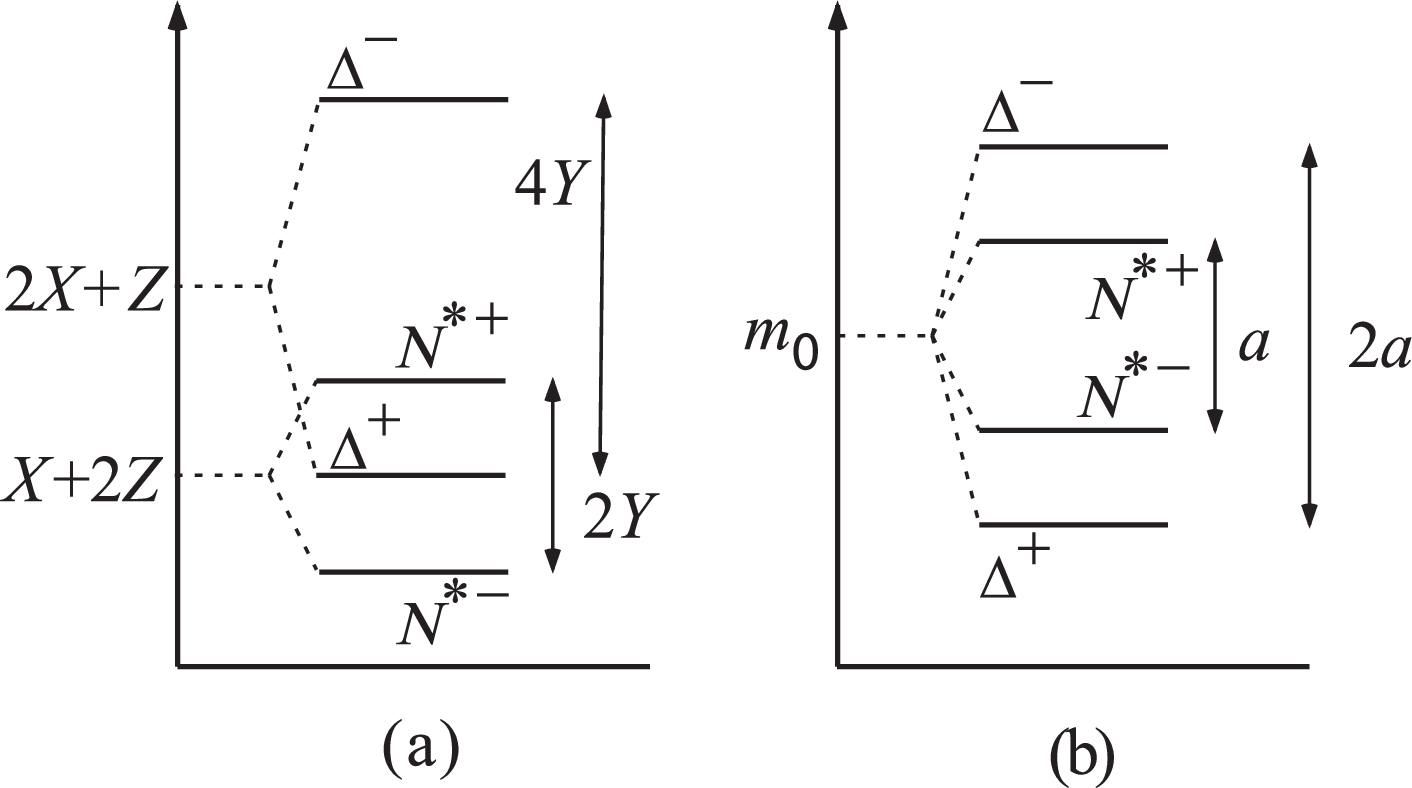
In order to understand their relation, we approximate the masses in two ways. In the small case, the masses are, up to , given by
where , and . In the dominant case, they are, up to , given by
where . The mass patterns for these cases are shown in Fig. 1. The two cases are different in the ordering of and . In the limit, they have mass ratio and is heavier than . Small values of do not change this ordering, which corresponds to the left panel in Fig. 1. When becomes much larger, the ordering is changed and becomes lowest-state. The cases (1) and (3-1) correspond to the mass pattern shown in the right panel in Fig. 1, while the cases (2) and (3-2) correspond to the left panel. Actually, is not small in the cases (2) and (3-2), but comparable to . However, the left panel in Fig. 1 well described the mass pattern of these cases. Using Eqs. (24) and (26), mixing angles in the small case takes moderate values and all the one-pion coupling constants survive. On the other hand in the -dominant case, mixing angles are and the parity-non-changing interactions vanish. Thus, the behavior of the one-pion coupling constants is related to the mass pattern of the quartet. According to this discussion, the cases (3-1) and (3-2) are different due to the ordering of and , although they describe the same assignments. This is the reason why the assignment , , , ) is sensitive to the choice of the experimental data. This discussion can be applied to other assignments we do not take into account. As we have mentioned, other three assignments reproduces the masses of the quartet with less than one :(, , , ), (, , , ), (, , , ). According to the above discussions, the first and second cases correspond to maximally-mixing with the vanishing of the parity-non-changing interactions, while all the coupling constants survive in the third case.
5 Summary
We have investigated the possibility that chiral partners exist in spin- baryon sector by considering the quartet scheme, where four spin- baryons, , , and , form the chiral multiplets with the mirror assignment. Using the Lagrangian, we tried to find a set of four baryons suitable for the chiral quartet. We discussed three assignments: (1) , (2) , (3-1) and (3-2) , , , ). Here we investigated , , , ) using two data sets.
For the case (1) we found that there is significant discrepancy for the masses, which implies the mass of is too small for the quartet scheme. In addition, the vanishing of inconsistent with other theories. Considering the discrepancy for the masses and the inconsistencies of , it seems that this case is less suitable for the quartet.
For the case (2), the masses of the observed baryons agree well with the mass pattern of the QS. Among all the possible assignments, the value becomes the smallest in this case. Considering the masses, this case is most suitable for the quartet. Regarding the interactions, this case does not reproduce reasonable results.
For the assignment , , , ), we consider two cases (3-1) and (3-2) with the use of different data sets because of the variety of the experimental data. Both cases reproduce the masses of the quartet with less than one. The one-pion coupling constants for this assignment are quite sensitive to the ordering of the masses of and . If the mass of is smaller than that of , only the parity-changing one-pion interactions survive. On the other hand, if the mass of is smaller, all the coupling constants are finite and the parity-non-changing interactions are larger than the parity-changing ones. Regarding the interactions, we obtained reasonable results for the case (3-2).
For further confirmation, experiments or lattice calculations for the one-pion coupling constants are needed. For instance, we can test the validity of the case (2) using coupling constants such as , and . For the further study of the assignment (, , , ), we need information about the masses because of a variety of the data. Especially, detailed information of the masses of and are needed, because the one-pion coupling constants are sensitive to the ordering of the masses of them. If the mass ordering are determined, we can test this assignment using one-pion coupling constants such as .
It is important to extend the present framework with the inclusion of higher-dimensional chiral representations for the nucleon. For the interactions with the quartet, we adopted the assumption that the nucleon belongs to the fundamental chiral representation. There are other possibilities for the nucleon’s chiral representation. Hence, the disagreements for the interactions may come from this assumption and can be resolved by including higher-dimensional chiral representations for the nucleon. Furthermore, it may be possible to test the nucleon’s chiral representations through the interactions with the quartet, if we can confirm the QS by using the one-pion interactions for the quartet.
In the present study, we employed the effective Lagrangian approach, where we truncated higher-order terms in the Lagrangian and we neglected quantum effects. With the high-lying baryons in the multiplet, we need to include various resonances in order to evaluate the quantum effects properly, which would cause additional difficulties. Rather, it is desired to reproduce and confirm the present result using different method. For instance, an algebraic method proposed by Weinberg is one of the useful method to study chiral partners. This method is based on the commutation relations derived from the superconvergence property of pion-nucleon scattering amplitudes, and can be applied to baryons [35, 36, 37]. We have already started a study along this line in Ref. [32].
Acknowledgments
This work was partly supported by Grant-in-Aid for Scientific Research on Innovative Areas(20105003) and Grant-in-Aid for Scientific Research (B20340055).
Appendix A Fierz Transformation
We show the derivation of Eqs. (3). We define totally anti-symmetric fields as linear combinations of Eqs. (2)
| (62a) | ||||
| (62b) | ||||
| where | ||||
| (62c) | ||||
| (62d) | ||||
| (62e) | ||||
| (62f) | ||||
The coefficients and are determined by the totally anti-symmetric condition, which is implemented by the anti-symmetric condition under the interchange between the second and third quark is given by
| (63) |
where denotes a baryon field obtained from the Fierz transformation of . Fierz transformation formula is given in Ref. [29]. This equation can be read as two kinds of the eigen-value problems : (a) for the vector space , and (b) for the vector space . The eigen-value problem (a) gives identities between the baryon operators
| (64a) | ||||
| (64b) | ||||
which reduce the number of the independent fields [29, 44, 45, 46]. The eigen-value problem (b) determines the values of the coefficients and
| (65a) | ||||
| (65b) | ||||
with which and are totally anti-symmetric. This determine the ratio between and in . It is convenient to replace by and and by with the use of Eqs. (64), which can be done without the change of chiral transformation properties of and . Finally, we obtain Eqs. (3).
Appendix B Alternative derivation of chiral properties
We show an alternative derivation of the chiral transformation properties of and the mass relation. Starting point is a standard definition of the transformation in terms of the chiral algebra between charges and fields. In general, the transformation is given by with generators and infinitesimal parameters for the transformation. We describe by product of the isovector and isospinor . For simplicity, we suppress the Lorentz indices in this section.
In the left- and right-handed representation, they correspond to and : transforms as under and under , while transforms under and under . Note that this field corresponds to and in Eq. (2). It is easy to check that , and consist of , , and , while and contain and . Jido et. al. employed and for the description of [34]. The chiral transformations of these fields are given by
where we have defined . Using and , we obtain and transformation properties
| (70) | ||||
| (71) |
Employing an isospurion formalism, and components are obtained by and . After the irreducible decomposition, we obtain
| (72a) | ||||
| (72b) | ||||
Here note that the coefficients differ from Eqs. (4). This is because and describe and , respectively. Using Eqs. (3) and (64), we obtain and . Substituting these relations into Eqs. (72), we reproduce Eqs. (4).
Considering the components, it is easy to show that the transformations of the and fields
where is the axial-transformation matrix Eq. (72) for components. We introduce the mass matrix for as with and being the masses of and . We also introduce the pion interaction matrix for their pseudo-scalar couplings. With chiral invariance, the matrices , and must obey
which leads to a double-commutation relation
| (79) |
This double-commutation relation gives , which reproduces the mass relation between and . Note that the double commutator Eq. (79) is the necessity condition of chiral invariance.
References
- [1] U. Vogl and W. Weise, Prog. Part. Nucl. Phys. 27, 195 (1991).
- [2] S. P. Klevansky, Rev. Mod. Phys. 64, 649 (1992).
- [3] T. Hatsuda and T. Kunihiro, Phys. Rept. 247, 221 (1994), [hep-ph/9401310].
- [4] T. D. Cohen, Nucl. Phys. A775, 89 (2006), [hep-ph/0605206].
- [5] L. Y. Glozman, Phys. Rev. Lett. 99, 191602 (2007), [0706.3288].
- [6] L. Y. Glozman, Phys. Rept. 444, 1 (2007), [hep-ph/0701081].
- [7] R. L. Jaffe, D. Pirjol and A. Scardicchio, Phys. Rept. 435, 157 (2006), [hep-ph/0602010].
- [8] Y. Nambu and G. Jona-Lasinio, Phys. Rev. 122, 345 (1961).
- [9] Y. Nambu and G. Jona-Lasinio, Phys. Rev. 124, 246 (1961).
- [10] J. I. Kapusta and E. V. Shuryak, Phys. Rev. D49, 4694 (1994), [hep-ph/9312245].
- [11] N. Ishii, W. Bentz and K. Yazaki, Phys. Lett. B301, 165 (1993).
- [12] N. Ishii, W. Bentz and K. Yazaki, Phys. Lett. B318, 26 (1993).
- [13] N. Ishii, Nucl. Phys. A689, 793 (2001), [nucl-th/0004063].
- [14] H. Mineo, W. Bentz, N. Ishii and K. Yazaki, Nucl. Phys. A703, 785 (2002), [nucl-th/0201082].
- [15] W. Bentz, T. Horikawa, N. Ishii and A. W. Thomas, Nucl. Phys. A720, 95 (2003), [nucl-th/0210067].
- [16] N. Ishii, W. Bentz and K. Yazaki, Nucl. Phys. A587, 617 (1995).
- [17] L. J. Abu-Raddad, A. Hosaka, D. Ebert and H. Toki, Phys. Rev. C66, 025206 (2002), [nucl-th/0206002].
- [18] K. Nagata and A. Hosaka, Prog. Theor. Phys. 111, 857 (2004), [hep-ph/0312161].
- [19] K. Nagata, A. Hosaka and L. J. Abu-Raddad, Phys. Rev. C72, 035208 (2005), [hep-ph/0408312].
- [20] K. Nagata and A. Hosaka, J. Phys. G32, 777 (2006), [hep-ph/0506193].
- [21] M. Gell-Mann and M. Levy, Nuovo Cim. 16, 705 (1960).
- [22] B. W. Lee, Gordon and Breach, New York,(1972).
- [23] C. DeTar and T. Kunihiro, Phys. Rev. D39, 2805 (1989).
- [24] D. Jido, Y. Nemoto, M. Oka and A. Hosaka, Nucl. Phys. A671, 471 (2000), [hep-ph/9805306].
- [25] D. Jido, M. Oka and A. Hosaka, Prog. Theor. Phys. 106, 873 (2001), [hep-ph/0110005].
- [26] H. Nagahiro, D. Jido and S. Hirenzaki, Phys. Rev. C80, 025205 (2009), [0811.4516].
- [27] S. Gallas, F. Giacosa and D. H. Rischke, 0907.5084.
- [28] C. Sasaki and I. Mishustin, arXiv:1005.4811[hep-ph].
- [29] K. Nagata, A. Hosaka and V. Dmitrasinovic, Mod. Phys. Lett. A23, 2381 (2008), [0705.1896].
- [30] K. Nagata, A. Hosaka and V. Dmitrasinovic, Phys. Rev. Lett. 101, 092001 (2008), [0804.3185].
- [31] H.-X. Chen, V. Dmitrasinovic, A. Hosaka, K. Nagata and S.-L. Zhu, Phys. Rev. D78, 054021 (2008), [0806.1997].
- [32] K. Nagata, arXiv:0812.3982[hep-ph].
- [33] V. Dmitrasinovic, A. Hosaka and K. Nagata, Mod. Phys. Lett. A25, 233 (2010), [0912.2372].
- [34] D. Jido, T. Hatsuda and T. Kunihiro, Phys. Rev. Lett. 84, 3252 (2000), [hep-ph/9910375].
- [35] S. Weinberg, Phys. Rev. 177, 2604 (1969).
- [36] S. R. Beane and U. van Kolck, J. Phys. G31, 921 (2005), [nucl-th/0212039].
- [37] A. Hosaka, D. Jido and M. Oka, arXiv:hep-ph/0112355.
- [38] T. R. Hemmert, B. R. Holstein and J. Kambor, J. Phys. G24, 1831 (1998), [hep-ph/9712496].
- [39] V. Pascalutsa, M. Vanderhaeghen and S. N. Yang, Phys. Rept. 437, 125 (2007).
- [40] M. Benmerrouche, R. M. Davidson and N. C. Mukhopadhyay, Phys. Rev. C39, 2339 (1989).
- [41] H. Haberzettl, arXiv:nucl-th/9812043.
- [42] V. Pascalutsa and R. Timmermans, Phys. Rev. C60, 042201 (1999), [nucl-th/9905065].
- [43] V. Pascalutsa and M. Vanderhaeghen, Phys. Lett. B636, 31 (2006), [hep-ph/0511261].
- [44] B. L. Ioffe, Nucl. Phys. B188, 317 (1981).
- [45] Y. Chung, H. G. Dosch, M. Kremer and D. Schall, Nucl. Phys. B197, 55 (1982).
- [46] D. Espriu, P. Pascual and R. Tarrach, Nucl. Phys. B214, 285 (1983).
- [47] Particle Data Group, C. Amsler et al., Phys. Lett. B667, 1 (2008).
- [48] CB-ELSA, I. Horn et al., Eur. Phys. J. A38, 173 (2008), [0806.4251].
- [49] G. Penner and U. Mosel, Phys. Rev. C66, 055211 (2002), [nucl-th/0207066].
- [50] V. A. Nikonov, A. V. Anisovich, E. Klempt, A. V. Sarantsev and U. Thoma, Phys. Lett. B662, 245 (2008), [0707.3600].
- [51] D. M. Manley and E. M. Saleski, Phys. Rev. D45, 4002 (1992).
- [52] G. E. Brown and W. Weise, Phys. Rept. 22, 279 (1975).
- [53] N. Fettes and U. G. Meissner, Nucl. Phys. A679, 629 (2001), [hep-ph/0006299].
- [54] S.-L. Zhu, Phys. Rev. C63, 018201 (2001), [nucl-th/0009062].
- [55] O. Krehl, C. Hanhart, S. Krewald and J. Speth, Phys. Rev. C62, 025207 (2000), [nucl-th/9911080].
- [56] S. Schneider, S. Krewald and U.-G. Meissner, Eur. Phys. J. A28, 107 (2006), [nucl-th/0603040].