跳到论文正文
W Papers独立论文阅读器 arXiv:1003.2824 论文正文 计算阅读时间 · 0%
引用这篇论文根据当前论文元数据生成,正式投稿前建议核对。


License: arXiv.org perpetual non-exclusive license
arXiv:1003.2824v3 [hep-ph] 16 Dec 2011

Antenna subtraction for gluon scattering at NNLO

Preprint:  IPPP/10/22

August 24, 2026
E. W. Nigel Glover Affiliation: Department of Physics, University of Durham, Durham, DH1 3LE, UK    Joao Pires Affiliation: E-mails: e.w.n.glover@durham.ac.uk, joao.pires@durham.ac.uk.
Abstract: 

We use the antenna subtraction method to isolate the double real radiation infrared singularities present in gluonic scattering amplitudes at next-to-next-to-leading order. The antenna subtraction framework has been successfully applied to the calculation of NNLO corrections to the 3-jet cross section and related event shape distributions in electron-positron annihilation. Here we consider processes with two coloured particles in the initial state, and in particular two-jet production at hadron colliders such as the Large Hadron Collider (LHC). We construct a subtraction term that describes the single and double unresolved contributions from the six-gluon tree-level process using antenna functions with initial state partons and show numerically that the subtraction term correctly approximates the matrix elements in the various single and double unresolved configurations.
August 24, 2026

Keywords: 
QCD, NNLO Computations, Hadronic Colliders, Jets

1 Introduction

In proton-proton collisions, the factorised form of the inclusive cross section is given by,

𝑑σ=∑i,j∫d​σ^i​j​fi​(ξ1)​fj​(ξ2)​d​ξ1ξ1​d​ξ2ξ2{\rm d}\sigma=\sum_{i,j}\int{\rm d}\hat{\sigma}_{ij}f_{i}(\xi_{1})f_{j}(\xi_{2})\frac{d\xi_{1}}{\xi_{1}}\frac{d\xi_{2}}{\xi_{2}}

where d​σ^i​j{\rm d}\hat{\sigma}_{ij} is the parton-level scattering cross section for parton ii to scatter off parton jj normalised to the hadron-hadron flux11 1 The partonic cross section normalised to the parton-parton flux is obtained by absorbing the inverse factors of ξ1\xi_{1} and ξ2\xi_{2} into d​σ^i​j{\rm d}\hat{\sigma}_{ij}. and the sum runs over the possible parton types ii and jj. The probability of finding a parton of type ii in the proton carrying a momentum fraction ξ\xi is described by the parton distribution function fi​(ξ)​d​ξf_{i}(\xi)d\xi. By applying suitable cuts, one can study more exclusive observables such as the transverse momentum distribution or rapidity distributions of the hard objects (jets or vector bosons, higgs bosons or other new particles) produced in the hard scattering. The leading-order (LO) prediction is a useful guide to the rough size of the cross section, but is usually subject to large uncertainties from the dependence on the unphysical renormalisation and factorisation scales, as well as possible mismatches between the (theoretical) parton-level and the (experimental) hadron-level.

Frequently, the theoretical prediction may be improved by including higher order perturbative predictions which have the effect of (a) reducing the renormalisation/factorisation scale dependence and (b) improving the matching of the parton level event topology with the experimentally observed hadronic final state [1]. The partonic cross section d​σ^i​j{\rm d}\hat{\sigma}_{ij} has the perturbative expansion

d​σ^i​j=d​σ^i​jL​O+(αs2​π)​d​σ^i​jN​L​O+(αs2​π)2​d​σ^i​jN​N​L​O+𝒪⁡(αs3){\rm d}\hat{\sigma}_{ij}={\rm d}\hat{\sigma}_{ij}^{LO}+\left(\frac{\alpha_{s}}{2\pi}\right){\rm d}\hat{\sigma}_{ij}^{NLO}+\left(\frac{\alpha_{s}}{2\pi}\right)^{2}{\rm d}\hat{\sigma}_{ij}^{NNLO}+{\cal O}(\alpha_{s}^{3}) (1)

where the next-to-leading order (NLO) and next-to-next-to-leading order (NNLO) strong corrections are identified. Any calculation of these higher-order corrections requires a systematic procedure for extracting the infrared singularities that arise when one or more final state particles become soft and/or collinear. These singularities are present in the real radiation contribution at next-to-leading order (NLO), and in double real radiation and mixed real-virtual contributions at next-to-next-to-leading order (NNLO).

For example, let us consider the mm-jet cross section. This is obtained by evaluating the tree-level cross section for processes with mm-partons in the final state (i.e. the processes involving (m+2)(m+2)-partons with two partons in the initial state), and requiring that each final state parton is identified as a jet by some jet algorithm. For simplicity, we will focus on the contribution involving only gluons and will therefore drop the parton labels. Suppose we now want to compute the mm-jet cross section to NLO. For this, we have to consider the real radiation cross section d​σ^R{\rm d}\hat{\sigma}^{R} with (m+1m+1)-partons in the final state, the one-loop correction d​σ^V{\rm d}\hat{\sigma}^{V} with mm-partons in the final state, and a mass factorisation counterterm d​σ^M​F{\rm d}\hat{\sigma}^{MF} to absorb the divergences arising from initial state collinear radiation into the parton densities:

d​σ^N​L​O=∫d​Φm+1d​σ^N​L​OR+∫d​Φmd​σ^N​L​OV+∫d​Φmd​σ^N​L​OM​F.\displaystyle{\rm d}\hat{\sigma}_{NLO}=\int_{{\rm d}\Phi_{m+1}}{\rm d}\hat{\sigma}^{R}_{NLO}+\int_{{\rm d}\Phi_{m}}{\rm d}\hat{\sigma}^{V}_{NLO}+\int_{{\rm d}\Phi_{m}}{\rm d}\hat{\sigma}^{MF}_{NLO}. (2)

Here the integration is over the appropriate NN-parton final state subject to the constraint that precisely mm-jets are observed by the jet algorithm Jm(N)J_{m}^{(N)},

∫d​ΦN≡∫dΦNJm(N).\int_{{\rm{d}}\Phi_{N}}\equiv\int{\rm{d}}\Phi_{N}J_{m}^{(N)}. (3)

The terms on the right hand side of (2) are separately divergent although their sum is finite. To write a Monte Carlo program to compute those integrals we must first isolate and cancel the singularities of the different pieces and then numerically evaluate the finite remainders to obtain the NLO contribution to the cross section.

Subtraction schemes are a well established solution to this problem. They work by finding a suitable counterterm d​σ^N​L​OS{\rm d}\hat{\sigma}^{S}_{NLO} for d​σ^N​L​OR{\rm d}\hat{\sigma}^{R}_{NLO}. It has to satisfy two properties, namely it must have the same singular behaviour in all appropriate limits as d​σ^N​L​OR{\rm d}\hat{\sigma}^{R}_{NLO} and yet be simple enough to be integrated analytically over all singular regions of the (m+1)(m+1)-parton phase space in dd dimensions. We proceed by rewriting (2) in the following form:

d​σ^N​L​O=∫d​Φm+1(d​σ^N​L​OR−d​σ^N​L​OS)+∫d​Φm(∫1d​σ^N​L​OS+d​σ^N​L​OV+d​σ^N​L​OM​F).\displaystyle{\rm d}\hat{\sigma}_{NLO}=\int_{{\rm d}\Phi_{m+1}}\left({\rm d}\hat{\sigma}_{NLO}^{R}-{\rm d}\hat{\sigma}_{NLO}^{S}\right)+\int_{{\rm d}\Phi_{m}}\left(\int_{1}{\rm d}\hat{\sigma}_{NLO}^{S}+{\rm d}\hat{\sigma}_{NLO}^{V}+{\rm d}\hat{\sigma}_{NLO}^{MF}\right). (4)

In its unintegrated form d​σ^N​L​OS{\rm d}\hat{\sigma}_{NLO}^{S} has the same singular behaviour as d​σ^N​L​OR{\rm d}\hat{\sigma}_{NLO}^{R} such that the first integral is finite by definition and can be integrated numerically in four dimensions over the (m+1)(m+1)-parton phase space. The integrated form of the counterterm d​σ^N​L​OS{\rm d}\hat{\sigma}_{NLO}^{S} analytically cancels the explicit singularities of the virtual contribution d​σ^N​L​OV{\rm d}\hat{\sigma}_{NLO}^{V} and the mass factorisation counterterm d​σ^N​L​OM​F{\rm d}\hat{\sigma}_{NLO}^{MF}. After checking the cancellation of the pole pieces, we can take the finite remainders of these contributions and perform the last integral on the right hand side of (4) numerically over the mm-parton phase space.

The actual form of the counterterm d​σ^N​L​OS{\rm d}\hat{\sigma}_{NLO}^{S} depends on the subtraction formalism employed because there are many ways of approximating the matrix elements in the neighbourhood of its soft and collinear singularities. Several methods for constructing NLO subtraction terms systematically have been proposed in the literature [2, 3, 4, 5, 6] and both the Catani-Seymour [2] and FKS [3] subtraction formalisms have been implemented in an automated way in [7, 8, 9, 10, 11, 12] and [13] respectively. These packages aim to automatically generate the subtraction terms and real emission amplitudes for any given process. Used in conjunction with recent automated packages that compute the virtual contribution [14, 15, 16, 17], there is the exciting possibility of having an automated NLO QCD parton level event generator available in the near future.

Nevertheless, for some processes, particularly the main 2→12\to 1 or 2→22\to 2 scattering processes such as Drell-Yan, Higgs production, di-jet production, vector-boson plus jet, vector-boson pair production or heavy quark pair production, the NLO corrections still have a large theoretical uncertainty and it is necessary to include the NNLO perturbative corrections. In addition to reducing the renormalisation and factorisation scale dependence there is an improved matching of the parton level theoretical jet algorithm with the hadron level experimental jet algorithm because the jet structure can be modeled by the presence of a third parton. For di-jet production, the resulting theoretical uncertainty at NNLO is estimated to be at the few per-cent level [1].

At NNLO, there are three distinct contributions due to double real radiation radiation d​σ^N​N​L​OR{\rm{d}}\hat{\sigma}_{NNLO}^{R}, mixed real-virtual radiation d​σ^N​N​L​OV,1{\rm{d}}\hat{\sigma}_{NNLO}^{V,1} and double virtual radiation d​σ^N​N​L​OV,2{\rm{d}}\hat{\sigma}_{NNLO}^{V,2}, that are given by

d​σ^N​N​L​O\displaystyle{\rm d}\hat{\sigma}_{NNLO} =\displaystyle= ∫d​Φm+2d​σ^N​N​L​OR+∫d​Φm+1d​σ^N​N​L​OV,1+∫d​Φmd​σ^N​N​L​OV,2\displaystyle\int_{{\rm{d}}\Phi_{m+2}}{\rm{d}}\hat{\sigma}_{NNLO}^{R}+\int_{{\rm{d}}\Phi_{m+1}}{\rm{d}}\hat{\sigma}_{NNLO}^{V,1}+\int_{{\rm{d}}\Phi_{m}}{\rm{d}}\hat{\sigma}_{NNLO}^{V,2} (5)

where the integration is over the appropriate NN-particle final state subject to the constraint that precisely mm-jets are observed. As usual the individual contributions in the mm, (m+1)(m+1) and (m+2)(m+2)-parton final states are all separately infrared divergent although, after renormalisation and factorisation, their sum is finite.

For processes with two partons in the initial state, the parton level cross sections are related to the interference of MM-particle ii-loop and jj-loop amplitudes [⟨ℳ(i)|ℳ(j)⟩]M[\langle{\cal M}^{(i)}|{\cal M}^{(j)}\rangle]_{M} by

d​σ^N​N​L​OR\displaystyle{\rm{d}}\hat{\sigma}_{NNLO}^{R} ∼\displaystyle\sim [⟨ℳ(0)|ℳ(0)⟩]m+4,\displaystyle\left[\langle{\cal M}^{(0)}|{\cal M}^{(0)}\rangle\right]_{m+4},
d​σ^N​N​L​OV,1\displaystyle{\rm{d}}\hat{\sigma}_{NNLO}^{V,1} ∼\displaystyle\sim [⟨ℳ(0)|ℳ(1)⟩+⟨ℳ(1)|ℳ(0)⟩]m+3,\displaystyle\left[\langle{\cal M}^{(0)}|{\cal M}^{(1)}\rangle+\langle{\cal M}^{(1)}|{\cal M}^{(0)}\rangle\right]_{m+3},
d​σ^N​N​L​OV,2\displaystyle{\rm{d}}\hat{\sigma}_{NNLO}^{V,2} ∼\displaystyle\sim [⟨ℳ(1)|ℳ(1)⟩+⟨ℳ(0)|ℳ(2)⟩+⟨ℳ(2)|ℳ(0)⟩]m+2.\displaystyle\left[\langle{\cal M}^{(1)}|{\cal M}^{(1)}\rangle+\langle{\cal M}^{(0)}|{\cal M}^{(2)}\rangle+\langle{\cal M}^{(2)}|{\cal M}^{(0)}\rangle\right]_{m+2}. (6)

In this paper, we specialise to the gluonic contributions to dijet production. Sample diagrams for each ingredient with m=2m=2 in the pure gluon channel is given in figure 1.

Refer to caption

ℳ6(0)​(g​g→g​g​g​g){\cal M}_{6}^{(0)}(gg\to gggg)      ℳ5(1)​(g​g→g​g​g){\cal M}_{5}^{(1)}(gg\to ggg)      ℳ4(2)​(g​g→g​g){\cal M}_{4}^{(2)}(gg\to gg)

Figure 1: Sample diagrams contributing to the dijet inclusive rate at NNLO

Explicit expressions for the interference of the four-gluon tree-level and two-loop amplitudes are available in Refs. [18, 19], while the self interference of the four-gluon one-loop amplitude is given in [20]. The remaining two-loop matrix elements, for quark-quark and quark-gluon scattering were obtained in [21, 22, 23, 24, 25]. These two-loop contributions contain explicit infrared divergences coming from the integration over the loop momentum. This singular behaviour is predictable with the Catani formula for the IR pole structure for a general on-shell QCD amplitude at two loop order derived in [26]. The one-loop helicity amplitudes for the five gluon amplitude are given in [27]. This contribution contains explicit infrared divergences coming from integrating over the loop momenta and implicit poles in the regions of the phase space where one of the final state partons becomes unresolved. This corresponds to the soft and collinear regions of the one-loop amplitude that were analyzed in [28, 29, 30]. The double real six-gluon matrix elements were derived in [31, 32, 33]. Here the singularities occur in the phase space regions corresponding to two gluons becoming simultaneously soft and/or collinear. The “double” unresolved behaviour is universal and was discussed in [34, 35, 36, 37].

Understanding the origin of the singularities of the different contributions is fundamental to constructing a subtraction procedure that can achieve their analytic cancellation. There have been several approaches to build a general subtraction scheme at NNLO [38, 39, 40, 41, 42, 43, 44, 45, 46, 47]. Another subtraction type scheme has been proposed in [48]. It is not a general NNLO subtraction scheme, but can nevertheless deal with an entire class of processes in hadron-hadron collisions and has been explicitly applied to several observables [48, 49, 50, 51]. In addition, there is the completely independent sector decomposition approach which avoids the need for analytical integration and which has been developed for virtual [52, 53, 54] and real radiation [55, 56, 57, 58] corrections to NNLO, and applied to several observables already [59, 60, 61, 62].

We will follow the NNLO antenna subtraction method which was derived in [38] for processes involving only (massless) final state partons. This formalism has been applied in the computation of NNLO corrections to three-jet production in electron-positron annihilation [63, 64, 65, 66] and related event shapes [67, 68, 69, 70, 71], which were subsequently used in precision determinations of the strong coupling constant [72, 73, 74, 75, 76]. It has also been extended at NNLO to include one hadron in the initial state relevant for electron-proton scattering [77, 78] while in ref. [79] the extension of the antenna subtraction method to include two hadrons in the initial state is discussed.

The general form for the subtraction terms for an mm-particle final state at NNLO is given by [38]:

d​σ^N​N​L​O\displaystyle{\rm d}\hat{\sigma}_{NNLO} =\displaystyle= ∫d​Φm+2(d​σ^N​N​L​OR−d​σ^N​N​L​OS)+∫d​Φm+2d​σ^N​N​L​OS\displaystyle\int_{{\rm{d}}\Phi_{m+2}}\left({\rm{d}}\hat{\sigma}_{NNLO}^{R}-{\rm{d}}\hat{\sigma}_{NNLO}^{S}\right)+\int_{{\rm{d}}\Phi_{m+2}}{\rm{d}}\hat{\sigma}_{NNLO}^{S} (7)
+\displaystyle+ ∫d​Φm+1(d​σ^N​N​L​OV,1−d​σ^N​N​L​OV​S,1)+∫d​Φm+1d​σ^N​N​L​OV​S,1+∫d​Φm+1d​σ^N​N​L​OM​F,1\displaystyle\int_{{\rm{d}}\Phi_{m+1}}\left({\rm{d}}\hat{\sigma}_{NNLO}^{V,1}-{\rm{d}}\hat{\sigma}_{NNLO}^{VS,1}\right)+\int_{{\rm{d}}\Phi_{m+1}}{\rm{d}}\hat{\sigma}_{NNLO}^{VS,1}+\int_{{\rm{d}}\Phi_{m+1}}{\rm{d}}\hat{\sigma}_{NNLO}^{MF,1}
+\displaystyle+ ∫d​Φmd​σ^N​N​L​OV,2+∫d​Φmd​σ^N​N​L​OM​F,2.\displaystyle\int_{{\rm{d}}\Phi_{m}}{\rm{d}}\hat{\sigma}_{NNLO}^{V,2}+\int_{{\rm{d}}\Phi_{m}}{\rm{d}}\hat{\sigma}_{NNLO}^{MF,2}.

Here, d​σ^N​N​L​OS{\rm d}\hat{\sigma}^{S}_{NNLO} denotes the subtraction term for the (m+2)(m+2)-parton final state which behaves like the double real radiation contribution d​σ^N​N​L​OR{\rm d}\hat{\sigma}^{R}_{NNLO} in all singular limits. Likewise, d​σ^N​N​L​OV​S,1{\rm d}\hat{\sigma}^{VS,1}_{NNLO} is the one-loop virtual subtraction term coinciding with the one-loop (m+1)(m+1)-final state d​σ^N​N​L​OV,1{\rm d}\hat{\sigma}^{V,1}_{NNLO} in all singular limits. The two-loop correction to the (m+2)(m+2)-parton final state is denoted by d​σ^N​N​L​OV,2{\rm d}\hat{\sigma}^{V,2}_{NNLO}. In addition, when there are partons in the initial state, there are two mass factorisation contributions, d​σ^N​N​L​OM​F,1{\rm d}\hat{\sigma}^{MF,1}_{NNLO} and d​σ^N​N​L​OM​F,2{\rm d}\hat{\sigma}^{MF,2}_{NNLO}, for the (m+1)(m+1)- and mm-particle final states respectively.

In this paper, we will develop the antenna subtraction method for two partons in the initial state. As a first example of how to use the formalism, we focus on the double real radiation contribution to dijet production in hadron-hadron collisions and specialise to the case where only gluons participate in the interaction. At NNLO, dijet production receives contributions from the double real six-gluon process. This particular contribution has the most complicated infrared structure that we can find at NNLO and we study that in detail.

Our paper is organised as follows. In section 2, we review the structure of the multi-gluon amplitudes and the associated multi-gluon cross sections. In section 3 we review the antenna method for gluons-only processes at NLO, and apply it to di-jet production in sect. 3.6. We develop the antenna subtraction terms for doubly unresolved radiation in section 4, and derive the subtraction terms for the six-gluon process in sect. 5. In section 6, we test the validity of the subtraction term by numerically studying the subtracted matrix elements in all of the singly- and doubly-unresolved limits. In particular, we show that in all cases the ratio of the double real cross section and the subtraction term approaches unity. Finally, our findings are summarised in section 7.

2 Gluonic amplitudes

The nn-gluon tree amplitude can be written as

𝐀n0({pi,λi,ai})=2n/2gn−2∑σ∈Sn/ZnTr(Taσ⁡(1)⋯Taσ⁡(n))𝒜n0(σ(1),⋯,σ(n))\displaystyle{\bf A}^{0}_{n}(\{p_{i},\lambda_{i},a_{i}\})=2^{n/2}g^{n-2}\sum_{\sigma\in S_{n}/Z_{n}}\textrm{Tr}(T^{a_{\sigma(1)}}\cdots T^{a_{\sigma(n)}}){\cal A}^{0}_{n}(\sigma(1),\cdots,\sigma(n))
(8)

where gg is the gauge coupling (g2=4​π​αsCLOSE({g^{2}}={4\pi}\alpha_{s}) and the permutation sum, Sn/ZnS_{n}/Z_{n} is the group of non-cyclic permutations of nn symbols. We will frequently denote the momentum pjp_{j} of gluon jj by jj. The helicity information is not relevant to the discussion of the subtraction terms and from now on, we will systematically suppress the helicity labels. The TaT^{a} are fundamental representation S​U​(N)SU(N) colour matrices, normalised such that Tr⁡(Ta​Tb)=δa​b/2{\rm Tr}(T^{a}T^{b})=\delta^{ab}/2.

ℳn​(1,⋯,n){\cal M}_{n}(1,\cdots,n) is the colour ordered partial amplitude [31, 80, 32, 33]. It is gauge invariant, as well as being invariant under cyclic permutations of the gluons.

The leading colour contribution to the squared matrix elements summed over colours (and helicities) is given by the sum of squares of partial amplitudes,

|𝐀n0|2=(g2​N)n−2​(N2−1)​∑σ∈Sn/Zn{|𝒜n0​(σ⁡(1),⋯,σ⁡(n))|2+𝒪⁡(1N2)}.\displaystyle|{\bf A}^{0}_{n}|^{2}=\left({g^{2}N}\right)^{n-2}(N^{2}-1)\sum_{\sigma\in S_{n}/Z_{n}}\left\{\ |{\cal A}^{0}_{n}(\sigma(1),\cdots,\sigma(n))|^{2}+{\cal O}\left(\frac{1}{N^{2}}\right)\right\}.

The infrared singularity properties of the tree-level colour ordered matrix elements have been well studied [81, 80, 34, 35, 36, 37, 82, 83, 84]. At tree-level, the colour-ordered gluon amplitude has a QED-like factorisation in the limit where gluon bb is soft, into an eikonal-type singular factor and a colour ordered tree-level squared amplitude where gluon bb has been removed. For the squared amplitude we have,

|𝒜n+10​(1,…,a,b,c,…,n+1)|2\displaystyle|{\cal A}^{0}_{n+1}(1,\ldots,a,b,c,\ldots,n+1)|^{2} ⟶bg→0\displaystyle\stackrel{{\scriptstyle b_{g}\to 0}}{{\longrightarrow}} Sa​b​c​|𝒜n​(1,…,a,c,…,n+1)|2,\displaystyle S_{abc}\;|{\cal A}_{n}(1,\ldots,a,c,\ldots,n+1)|^{2}, (10)

with the eikonal factor given by,

Sa​b​c=2​sa​csa​b​sb​c.\displaystyle S_{abc}=\frac{2s_{ac}}{s_{ab}s_{bc}}. (11)

Similarly in the limit where two gluons become collinear, the colour-ordered amplitudes factorise. If gluons aa and bb become collinear and form gluon cc, then adjacent gluons give a singular contribution,

|𝒜n+10​(1,…,a,b,…,n+1)|2\displaystyle|{\cal A}^{0}_{n+1}(1,\ldots,a,b,\ldots,n+1)|^{2} ⟶a//b\displaystyle\stackrel{{\scriptstyle a//b}}{{\longrightarrow}} 1sa​b​Pg​g→g​(z)​|𝒜n0​(1,…,c,…,n+1)|2\displaystyle\frac{1}{s_{ab}}P_{gg\to g}(z)|{\cal A}^{0}_{n}(1,\ldots,c,\ldots,n+1)|^{2}

while separated gluons do not,

|𝒜n+10​(1,…,a,…,b,…,n+1)|2\displaystyle|{\cal A}^{0}_{n+1}(1,\ldots,a,\ldots,b,\ldots,n+1)|^{2} ⟶a//b\displaystyle\stackrel{{\scriptstyle a//b}}{{\longrightarrow}} finite.\displaystyle\textrm{finite}. (13)

In equation (), zz is the fraction of momentum carried by one of the gluons and, after integrating over the azimuthal angle of the plane containing the collinear particles with respect to the hard process, collinear splitting function Pg​g→gP_{gg\to g} is given by,

Pg​g→g​(z)=2​(z1−z+1−zz+z⁡(1−z)).\displaystyle P_{gg\to g}(z)=2\left(\frac{z}{1-z}+\frac{1-z}{z}+z(1-z)\right). (14)

In the case of two real unresolved particles there are a variety of different configurations extensively studied in [34, 35, 36, 37]. The expressions for these universal limits are organised according to whether the two unresolved particles are colour connected or not. In the unconnected case, i.e. where the gluons are not adjacent in the colour ordered amplitude, the singular limits are merely obtained by multiplying single unresolved factors. However, when the particles are colour connected, i.e. where the gluons are adjacent in the colour ordered amplitude, the structure is more involved.

At higher numbers of loops, the leading colour contribution to the nn-gluon mm-loop amplitude can be written as [85],

𝐀nm({pi,λi,ai})=2n/2gn−2+2​mNm∑σ∈Sn/ZnTr(Taσ⁡(1)⋯Taσ⁡(n))𝒜nm(σ(1),⋯,σ(n)).\displaystyle{\bf A}^{m}_{n}(\{p_{i},\lambda_{i},a_{i}\})=2^{n/2}g^{n-2+2m}N^{m}\sum_{\sigma\in S_{n}/Z_{n}}\textrm{Tr}(T^{a_{\sigma(1)}}\cdots T^{a_{\sigma(n)}}){\cal A}^{m}_{n}(\sigma(1),\cdots,\sigma(n)). (15)

The single unresolved infrared singularity structure of one- and two-loop amplitudes has been studied in Refs. [85, 28, 86, 87, 29, 30, 88, 89, 90, 91, 92].

For convenience, we introduce the additional notation

AnM(σ(1),…,σ(n))=∑helicities∑i=0..M𝒜ni†(σ(1),…,σ(n))𝒜nM−i(σ(1),…,σ(n)).{A}^{M}_{n}(\sigma(1),\ldots,\sigma(n))=\sum_{\rm helicities}\sum_{i=0..M}{\cal A}_{n}^{i\dagger}(\sigma(1),\ldots,\sigma(n)){\cal A}_{n}^{M-i}(\sigma(1),\ldots,\sigma(n)). (16)

We will encounter A50{A}_{5}^{0} and A41{A}_{4}^{1} in the example of the antenna subtraction at NLO given in sections 3.6.1 and 3.6.2 respectively, while A60{A}^{0}_{6}, A51{A}^{1}_{5} and A42{A}^{2}_{4} are relevant for the NNLO dijet cross section. In section 4.6, we will explicitly derive the NNLO subtraction term for A60{A}^{0}_{6}.

3 Antenna subtraction at NLO

The leading-order parton-level contribution from the (m+2)(m+2)-parton processes to the mm-jet cross section at LO in p​ppp collisions is given by

d​σ^L​O\displaystyle{\rm d}\hat{\sigma}_{LO} =\displaystyle= 𝒩​∑permsd​Φm​(p3,…,pm+2,p1,p2)​1Sm\displaystyle{\cal N}\sum_{\textrm{perms}}{\rm d}\Phi_{m}(p_{3},\ldots,p_{m+2};p_{1},p_{2})\frac{1}{S_{m}} (17)
×|ℳm+2​(1,…,m+2)|2​Jm(m)​(p3,…,pm+2)\displaystyle\times|{\cal M}_{m+2}(1,\ldots,m+2)|^{2}J_{m}^{(m)}(p_{3},\ldots,p_{m+2})

where to make the subsequent discussion more general, we denote a generic tree-level colour ordered amplitude by the symbol ℳ⁡(1,…,m+2){\cal M}(1,\ldots,m+2). The sum over perms{\rm perms} is the appropriate sum over colour ordered amplitudes. For gluonic amplitudes this is the sum over the group of non-cyclic permutations of nn symbols denoted by Sn/ZnS_{n}/Z_{n} in the previous section. The symmetry factor SmS_{m} accounts for identical partons in the final state. The normalisation factor 𝒩{\cal N} includes all QCD-independent factors as well as the dependence on the renormalised QCD coupling constant αs\alpha_{s}. The initial state momenta are labeled as usual as p1p_{1} and p2p_{2} whereas the mm-momenta in the final state are labeled p3,…,pm+2p_{3},\ldots,p_{m+2}. d​Φm{\rm d}\Phi_{m} is the 2→m2\to m particle phase space:

d​Φm​(p3,…,pm+2,p1,p2)=\displaystyle{\rm d}\Phi_{m}(p_{3},\ldots,p_{m+2};p_{1},p_{2})=
dd−1​p32​E3​(2​π)d−1​…​dd−1​pm+22​Em+2​(2​π)d−1​(2​π)d​δd​(p1+p2−p3−…−pm+2).\displaystyle\frac{{\rm d}^{d-1}p_{3}}{2E_{3}(2\pi)^{d-1}}\ldots\frac{{\rm d}^{d-1}p_{m+2}}{2E_{m+2}(2\pi)^{d-1}}(2\pi)^{d}\delta^{d}(p_{1}+p_{2}-p_{3}-\ldots-p_{m+2}). (18)

The jet function Jm(m)​(p3,…,pm+2)J_{m}^{(m)}(p_{3},\ldots,p_{m+2}) defines the procedure for building mm-jets from (mm)-partons. The main property of Jm(m)J_{m}^{(m)} is that the jet observable defined above is collinear and infrared safe.

We now focus on the antenna subtraction at NLO [93, 38, 94, 95]. In this approach, antenna functions describe the colour-ordered radiation of unresolved partons between a pair of hard (radiator) partons. We must distinguish three possible configurations of radiators: final-final when both radiators are final state partons, initial-final when one radiator is an initial state parton and the other radiator is a final state parton and, finally, initial-initial where both radiators are initial state partons.

This means that we will derive subtraction formulae decomposed in these three configurations and label them with a superscript (f​f),(i​f),(i​i)(ff),(if),(ii). In table 1 we distinguish the configurations that are needed according to the scattering process that we are interested in.

final-final initial-final initial-initial
e+​e−e^{+}e^{-} ✓ ✗ ✗
e​pep ✓ ✓ ✗
p​ppp ✓ ✓ ✓
Table 1: Antennae configurations needed according to the scattering process

Even though we will write down all formulae specifically for p​ppp collisions these formulae can be easily adapted to e​pep or e+​e−e^{+}e^{-} for the configurations they have in common. To achieve that we should only modify the number of partons that enter the matrix elements in these formulae. This is because we obtain an mm-jet production at leading order from an mm-parton matrix element in e+​e−e^{+}e^{-}, an (m+1m+1)-parton matrix element in e​pep and an (m+2m+2)-parton matrix element in p​ppp.

The mm-jet real radiation cross section at NLO in p​ppp collisions is given by,

d​σ^N​L​OR\displaystyle{\rm d}\hat{\sigma}_{NLO}^{R} =\displaystyle= 𝒩​∑permsd​Φm+1​(p3,…,pm+3,p1,p2)​1Sm+1\displaystyle{\cal N}\sum_{\textrm{perms}}{\rm d}\Phi_{m+1}(p_{3},\ldots,p_{m+3};p_{1},p_{2})\frac{1}{S_{m+1}} (19)
×|ℳm+3​(1,…,m+3)|2​Jm(m+1)​(p3,…,pm+3).\displaystyle\times|{\cal M}_{m+3}(1,\ldots,m+3)|^{2}J_{m}^{(m+1)}(p_{3},\ldots,p_{m+3}).

3.1 Final-Final configuration

When summing over all colour orderings in equation (19) we find terms of this type:

|ℳm+3​(…,i,j,k,…)|2\displaystyle|{\cal M}_{m+3}(\ldots,i,j,k,\ldots)|^{2} (20)

where i,j,ki,j,k are colour connected final state partons. This configuration contains a singularity when jj is unresolved between ii and kk which can be approximated by,

Xi​j​k​|ℳm+2​(…,I,K,…)|2,\displaystyle X_{ijk}|{\cal M}_{m+2}(\ldots,I,K,\ldots)|^{2}, (21)

where Xi​j​kX_{ijk} is a final-final antenna function that describes all singular configurations (for this colour-ordered amplitude) where parton jj is unresolved. The momenta for the new partons II and JJ are linear combinations of pip_{i}, pjp_{j}, pkp_{k} obtained with a final-final mapping that we describe in section 3.5.1. Both radiator partons ii and kk are in the final state and we call this situation a final-final antenna, depicted in figure 2. We still have to sum over all possible unresolved partons in this colour ordered amplitude. After that we sum over all colour orderings to obtain the full subtraction term, for the final-final configuration, to use with (19). The subtraction term for this configuration reads:

d​σ^S,(f​f)=𝒩​∑permsd​Φm+1​(p3,…,pm+3,p1,p2)​1Sm+1\displaystyle{\rm d}\hat{\sigma}^{S,(ff)}={\cal N}\sum_{\textrm{perms}}{\rm d}\Phi_{m+1}(p_{3},\ldots,p_{m+3};p_{1},p_{2})\frac{1}{S_{m+1}}
×∑jXi​j​k0​|ℳm+2​(…,I,K,…)|2​Jm(m)​(p3,…,pI,pK,…,pm+3).\displaystyle\times\sum_{j}X_{ijk}^{0}|{\cal M}_{m+2}(\ldots,I,K,\ldots)|^{2}J_{m}^{(m)}(p_{3},\ldots,p_{I},p_{K},\ldots,p_{m+3}). (22)

The subtraction term involves an (m+2)(m+2)-parton amplitude that does not depend on pip_{i}, pjp_{j}, pkp_{k} but on the redefined on-shell momenta pIp_{I} and pKp_{K}, where pIp_{I} and pKp_{K} are linear combinations of pip_{i}, pjp_{j}, pk{p}_{k}, while the tree antenna function Xi​j​k0X^{0}_{ijk} depends only on pip_{i}, pjp_{j} and pkp_{k}.

Refer to caption
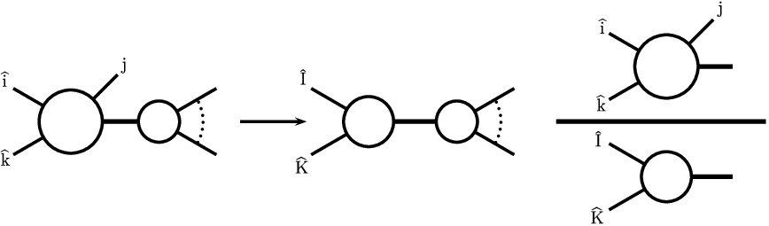
Figure 2: Illustration of NLO antenna factorisation representing the factorisation of both the squared matrix elements and the (m+1)(m+1)-particle phase space when the unresolved particle jj is colour connected between two final state radiators ii and kk.

The jet function Jm(m)J^{(m)}_{m} in (22) does not depend on the individual momenta pi{p}_{i}, pjp_{j} and pk{p}_{k}, but only on pIp_{I} and pKp_{K}. One can therefore carry out the integration over the unresolved dipole phase space appropriate for pi{p}_{i}, pjp_{j} and pk{p}_{k} analytically, exploiting the factorisation of the phase space,

d​Φm+1​(p3,…,pm+3,p1,p2)=\displaystyle{\rm d}\Phi_{m+1}(p_{3},\ldots,p_{m+3};p_{1},p_{2})= (23)
d​Φm​(p3,…,pI,pK,…,pm+3,p1,p2)⋅d​ΦXi​j​k​(pi,pj,pk,pI+pK).\displaystyle{\rm d}\Phi_{m}(p_{3},\ldots,p_{I},p_{K},\ldots,p_{m+3};p_{1},p_{2})\cdot{\rm d}\Phi_{X_{ijk}}(p_{i},p_{j},p_{k};p_{I}+p_{K}).

The NLO antenna phase space d​ΦXi​j​k{\rm d}\Phi_{X_{ijk}} is proportional to the three-particle phase space relevant to a 1→31\to 3 decay.

For the analytic integration, we can use (23) to rewrite each of the subtraction terms in (22) in the form,

|ℳm+2|2​Jm(m)​d​Φm​∫d​ΦXi​j​k​Xi​j​k0.|{\cal M}_{m+2}|^{2}\,J_{m}^{(m)}\;{\rm d}\Phi_{m}\int{\rm d}\Phi_{X_{ijk}}\;X^{0}_{ijk}.

The analytic integral of the subtraction term is therefore defined as the antenna function integrated over the fully inclusive antenna phase space, normalised appropriately,

𝒳i​j​k0​(si​j​k)=1C⁡(ϵ)​∫d​ΦXi​j​k​Xi​j​k0,{\cal X}^{0}_{ijk}(s_{ijk})=\frac{1}{C(\epsilon)}\int{\rm d}\Phi_{X_{ijk}}\;X^{0}_{ijk}, (24)

where

C⁡(ϵ)=(4​π)ϵ​e−ϵ​γ8​π2.C(\epsilon)=(4\pi)^{\epsilon}\frac{e^{-\epsilon\gamma}}{8\pi^{2}}. (25)

The integration is performed analytically in dd dimensions to make the infrared singularities explicit and then added directly to the one-loop mm-particle contribution d​σ^N​L​OV{\rm d}\hat{\sigma}^{V}_{NLO}.

3.2 Initial-Final configuration

In the presence of hadrons in the initial state, matrix elements exhibit singularities that are not accounted by the subtraction terms discussed in the previous section. These singularities are due to soft or collinear radiation within an antenna where one or the two hard partons are in the initial state [94]. This occurs in equation (19) when in the ordered amplitude parton jj is unresolved between an initial state parton i^\hat{i} and a final state parton kk,

|ℳm+3​(…,i^,j,k,…)|2.|{\cal M}_{m+3}(\ldots,\hat{i},j,k,\ldots)|^{2}. (26)

Here and subsequently, a hat denotes an initial state parton. The infrared singularities can be approximated by,

Xi,j​k​|ℳm+2​(…,I^,K,…)|2X_{i,jk}|{\cal M}_{m+2}(\ldots,\hat{I},K,\ldots)|^{2} (27)

where Xi,j​kX_{i,jk} is an initial-final antenna function that describes configurations (for this colour-ordered amplitude) where parton jj is unresolved. This configuration is depicted in figure 3. The mapping that generates the new momenta pKp_{K} and pI^p_{\hat{I}} (which is simply a rescaling of incoming momentum pip_{i} by an amount xx such that pI^≡p¯i=xi​pi,p_{\hat{I}}\equiv\bar{p}_{i}=x_{i}p_{i},) will be discussed in 3.5.2. The full subtraction term for the the initial-final configuration reads,

d​σ^S,(i​f)=𝒩​∑permsd​Φm+1​(p3,…,pm+3,p1,p2)​1Sm+1\displaystyle{\rm d}\hat{\sigma}^{S,(if)}={\cal N}\sum_{\textrm{perms}}{\rm d}\Phi_{m+1}(p_{3},\dots,p_{m+3};p_{1},p_{2})\,\frac{1}{S_{m+1}}
×∑i=1,2∑jXi,j​k0​|ℳm+2​(…,I^,K,…)|2​Jm(m)​(p3,…,pK,…,pm+3).\displaystyle\times\sum_{i=1,2}\sum_{j}X^{0}_{i,jk}\left|{\cal M}_{m+2}(\ldots,\hat{I},K,\ldots)\right|^{2}\,J^{(m)}_{m}(p_{3},\ldots,p_{K},\ldots,p_{m+3}). (28)

The terms necessary to subtract singularities associated with coloured particles in the initial state can then be simply obtained by crossing the corresponding antennae for final state singularities (Xi​j​k→Xi,j​kX_{ijk}\to X_{i,jk}). Due to the different kinematics involved, the factorisation of the phase space is slightly more involved and the corresponding phase space mappings are different. To cancel explicit infrared poles in virtual contributions and in terms arising from parton distribution mass factorisation, the crossed antennae must be integrated, analytically, over the corresponding phase space.

Refer to caption
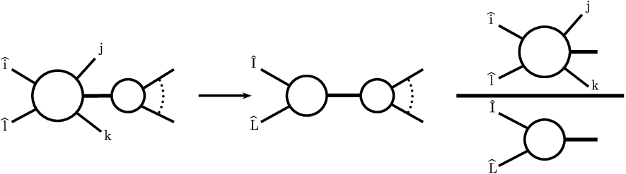
Figure 3: Illustration of NLO antenna factorisation representing the factorisation of both the squared matrix elements and the (m+1)(m+1)-particle phase space when the unresolved particle jj is colour connected between an initial state radiator i^\hat{i} and a final state radiator kk.

As in the final-final case, the tree antenna, Xi,j​k0X^{0}_{i,jk}, depends only on the original momenta pip_{i}, pjp_{j} and pkp_{k}, and contains all the configurations in which parton jj becomes unresolved. Similarly, the (m+2)(m+2)-parton amplitude depends only on the redefined on-shell momenta pI^p_{\hat{I}} (and therefore on the momentum fraction xx) and pKp_{K} and not on pip_{i}, pjp_{j} and pkp_{k}. The jet function, Jm(m)J^{(m)}_{m} depends on the momenta pip_{i}, pjp_{j} and pkp_{k} only through pKp_{K}. Thus, provided a suitable factorisation of the phase space, one can perform the integration of the antennae analytically.

The phase space can be factorised as an mm-parton phase space convoluted with a two particle phase space [94] such as the special case i=2i=2,

d​Φm+1​(p3,…,pm+3,p1,p2)\displaystyle{\rm d}\Phi_{m+1}(p_{3},\dots,p_{m+3};p_{1},p_{2}) =\displaystyle= d​Φm​(p3,…,pK,…,pm+3,p1,x2​p2)\displaystyle{\rm d}\Phi_{m}(p_{3},\dots,p_{K},\dots,p_{m+3};p_{1},x_{2}p_{2}) (29)
×\displaystyle\times Q22​π​d​Φ2​(pj,pk,p2,q)​d​x2x2\displaystyle\frac{Q^{2}}{2\pi}{\rm d}\Phi_{2}(p_{j},p_{k};p_{2},q)\frac{{\rm d}x_{2}}{x_{2}}\,

with Q2=−q2Q^{2}=-q^{2} and q=pj+pk−p2q=p_{j}+p_{k}-p_{2}. Replacing the phase space in (28), we can explicitly carry out the integration of the antenna factors over the two particle phase space. When combining the integrated subtraction terms with virtual contributions and mass factorisation terms, it turns out to be convenient to normalise the integrated antennae as follows

𝒳i,j​k​(xi)=1C⁡(ϵ)​∫d​Φ2​Q22​π​Xi,j​k,{\cal X}_{i,jk}(x_{i})=\frac{1}{C(\epsilon)}\int{\rm d}\Phi_{2}\frac{Q^{2}}{2\pi}X_{i,jk}\,, (30)

where C⁡(ϵ)C(\epsilon) is given in (25).

3.3 Initial-Initial configuration

The last situation to be considered is when the two hard radiators are in the initial state. The contribution from

|ℳm+3​(…,i^,j,k^,…)|2|{\cal M}_{m+3}(\ldots,\hat{i},j,\hat{k},\ldots)|^{2} (31)

contains the infrared singularities due to the unresolved parton jj when it is colour connected to both of the initial state partons i^\hat{i} and k^\hat{k}. As sketched in 4, these singularities can be approximated by,

Xi​k,j​|ℳm+2​(…,I^,K^,…)|2X_{ik,j}|{\cal M}_{m+2}(\ldots,\hat{I},\hat{K},\ldots)|^{2} (32)

where Xi​k,jX_{ik,j} is an initial-initial antenna function that describes configurations (for this colour-ordered amplitude) where parton jj is unresolved. In this case, the momentum mapping is more complicated, and not only are incoming momentum rescaled by an amount such that

pI^=xi​pi,pK^=xk​pk,{p_{\hat{I}}}=x_{i}p_{i},\qquad\qquad{p_{\hat{K}}}=x_{k}p_{k}, (33)

but all other spectator momenta must be Lorentz boosted to preserve momentum conservation,

pℓ→p~ℓ,ℓ≠i,j,k.p_{\ell}\to\tilde{p}_{\ell},\qquad\ell\neq i,j,k. (34)

The definitions of xix_{i} and xkx_{k} as well as the precise definition of the spectator momenta p~ℓ\tilde{p}_{\ell} will be discussed in section 3.5.3.

Refer to caption
Figure 4: Illustration of NLO antenna factorisation representing the factorisation of both the squared matrix elements and the (m+1)(m+1)-particle phase space when the unresolved particle jj is colour connected between two initial state radiators i^\hat{i} and k^\hat{k}.

The full subtraction term for the initial-initial configuration can be written as:

d​σ^S,(i​i)\displaystyle{\rm d}\hat{\sigma}^{S,(ii)} =\displaystyle= 𝒩​∑permsd​Φm+1​(p3,…,pm+3,p1,p2)​1Sm+1\displaystyle{\cal N}\sum_{\textrm{perms}}{\rm d}\Phi_{m+1}(p_{3},\ldots,p_{m+3};p_{1},p_{2})\,\frac{1}{S_{m+1}} (35)
∑i,k=1,2∑jXi​k,j0​|ℳm+2​(…,I^,K^,…)|2​Jm(m)​(p~3,…,p~m+3).\displaystyle\sum_{i,k=1,2}\sum_{j}X^{0}_{ik,j}\left|{\cal M}_{m+2}(\ldots,{\hat{I}},{\hat{K}},\ldots)\right|^{2}J^{(m)}_{m}(\tilde{p}_{3},\ldots,\tilde{p}_{m+3})\,.

In order to fulfill overall momentum conservation all the momenta in the arguments of the reduced matrix elements and the jet functions have been redefined.

The phase space factorises into the convolution of an mm particle phase space, involving only the redefined momenta, with the phase space of parton jj [94] so that when i=1i=1 and k=2k=2,

d​Φm+1​(p3,…,pm+3,p1,p2)\displaystyle{\rm d}\Phi_{m+1}(p_{3},\dots,p_{m+3};p_{1},p_{2}) =\displaystyle= d​Φm​(p~3,…,p~m+3,x1​p1,x2​p2)\displaystyle{\rm d}\Phi_{m}(\tilde{p}_{3},\ldots,\tilde{p}_{m+3};x_{1}p_{1},x_{2}p_{2}) (36)
×δ⁡(x1−x^1)​δ​(x2−x^2)​[d​pj]​d​x1​d​x2,\displaystyle\times\delta(x_{1}-\hat{x}_{1})\,\delta(x_{2}-\hat{x}_{2})\,[{\rm d}p_{j}]\,{\rm d}x_{1}\,{\rm d}x_{2}\,,

where the single particle phase space measure is [d​pj]=dd−1​pj/2​Ej​(2​π)d−1[{\rm d}p_{j}]={{\rm d}^{d-1}p_{j}}/{2E_{j}(2\pi)^{d-1}}.

Inserting the factorised expression for the phase space measure in eq. (35), the subtraction terms can be integrated over the antenna phase space [94]. The integrated form of the subtraction terms must be, then, combined with the virtual and mass factorisation terms to cancel the explicit poles in ϵ\epsilon. In the case of initial-initial subtraction terms, the antenna phase space is trivial: the two remaining Dirac delta functions can be combined with the one particle phase space, such that there are no integrals left. We define the initial-initial integrated antenna functions by,

𝒳i​k,j​(xi,xk)=1C⁡(ϵ)​∫[d​pj]​xi​xk​δ​(xi−x^i)​δ​(xk−x^k)​Xi​k,j{\cal X}_{ik,j}(x_{i},x_{k})=\frac{1}{C(\epsilon)}\int[{\rm d}p_{j}]\,x_{i}\,x_{k}\,\delta(x_{i}-\hat{x}_{i})\,\delta(x_{k}-\hat{x}_{k})\,X_{ik,j}\; (37)

where C⁡(ϵ)C(\epsilon) is given in (25).

3.4 Antenna functions

In the previous subsections we have seen that the subtraction term is constructed from products of antenna functions with reduced matrix elements (with fewer final state partons than the original matrix element), and integrated over a phase space which is factorised into an antenna phase space (involving all unresolved partons and the two radiators) multiplied with a reduced phase space (where the momenta of radiators and unresolved radiation are replaced by two redefined momenta). The full subtraction term is obtained by summing over all antennae required for the problem under consideration. In the most general case (two partons in the initial state, and two or more hard partons in the final state), this sum includes final-final, initial-final and initial-initial antennae. We will see an example of this in section 3.6.1 when we compute the NLO corrections to the dijet cross section.

The relevant antenna is determined by both the external state and the pair of hard partons it collapses to. In general we denote the antenna function as XX. For antennae that collapse onto a hard quark-antiquark pair, X=AX=A for q​g​q¯qg\bar{q}. Similarly, for quark-gluon antenna, we have X=DX=D for q​g​gqgg and X=EX=E for q​q′​q¯′qq^{\prime}\bar{q}^{\prime} final states. Finally, we characterise the gluon-gluon antennae as X=FX=F for g​g​gggg, X=GX=G for g​q​q¯gq\bar{q} final states.

At NLO, we only need to consider tree level three-particle antennae involving only one unresolved parton. At NNLO we will need four-particle antennae involving two unresolved partons and one-loop three-particle antennae.

In all cases the antenna functions are derived from physical matrix elements: the quark-antiquark antenna functions from γ∗→q​q¯+\gamma^{*}\to q\bar{q}~+ (partons) [96], the quark-gluon antenna functions from χ~→g~+\tilde{\chi}\to\tilde{g}~+ (partons) [97] and the gluon-gluon antenna functions from H→H\to (partons) [98]. The tree-level antenna functions are obtained by normalising the colour-ordered three- and four-parton tree-level squared matrix elements to the squared matrix element for the basic two-parton process,

Xi​j​k0=Si​j​k,I​K​|ℳi​j​k0|2|ℳI​K0|2,\displaystyle X_{ijk}^{0}=S_{ijk,IK}\,\frac{|{\cal M}^{0}_{ijk}|^{2}}{|{\cal M}^{0}_{IK}|^{2}}\;,
Xi​j​k​l0=Si​j​k​l,I​L​|ℳi​j​k​l0|2|ℳI​L0|2,\displaystyle X_{ijkl}^{0}=S_{ijkl,IL}\,\frac{|{\cal M}^{0}_{ijkl}|^{2}}{|{\cal M}^{0}_{IL}|^{2}}\;, (38)

where SS denotes the symmetry factor associated with the antenna, which accounts both for potential identical particle symmetries and for the presence of more than one antenna in the basic two-parton process.

Note that in the colour-ordered quark-gluon and gluon-gluon antenna functions derived from physical matrix elements for neutralino decay [97] and Higgs boson decay [98], it is in general not possible to identify the hard radiators and the unresolved partons in a unique manner. The reason for this ambiguity is in the cyclic nature of the colour orderings, which is already evident in the three-parton antenna functions: each pair of two partons can in principle act as hard radiators, resulting in more than one antenna configuration present in a single antenna function. This means that we have to disentangle the multiple singularities of these antennae into sub-antennae where an appropriate mapping can be used.

3.5 NLO antennae decomposition for numerical implementation

We will concentrate on the pure gluon channel and describe the numerical implementation of the gluon-gluon antenna function with a pure gluonic final state F30F_{3}^{0}. For that we will develop in the next subsections a further decomposition of the three parton gluon-gluon-gluon antenna function into different sub-antenna configurations for the different configurations of two emitters in the final-state (final-final emitters configuration), one emitter in the final state and one emitter in the initial state (initial-final emitters configuration) and both emitters in the initial state (initial-initial emitters configuration). The unresolved particle is always in the final state.

These three configurations are needed so that we can subtract the IR singularities from final-state radiation and initial state radiation. The different sub-antennae derived then will each contain singular limits appropriate to the phase-space mapping used in the three different configurations mentioned and all are extensively used in the subtraction terms at NLO and NNLO.

3.5.1 Final-Final emitters

The tree level three parton antenna corresponding to the gluon-gluon-gluon final state is [38]:

F30​(1g,2g,3g)\displaystyle F_{3}^{0}(1_{g},2_{g},3_{g}) =\displaystyle= 2s1232​(s1232​s12s13​s23+s1232​s13s12​s23+s1232​s23s12​s13+s12​s13s23+s12​s23s13+s13​s23s12CLOSE\displaystyle\frac{2}{s_{123}^{2}}\Bigg(\frac{s_{123}^{2}s_{12}}{s_{13}s_{23}}+\frac{s_{123}^{2}s_{13}}{s_{12}s_{23}}+\frac{s_{123}^{2}s_{23}}{s_{12}s_{13}}+\frac{s_{12}s_{13}}{s_{23}}+\frac{s_{12}s_{23}}{s_{13}}+\frac{s_{13}s_{23}}{s_{12}} (39)
OPEN+4​s123+𝒪⁡(ϵ))\displaystyle+4s_{123}+{\cal O}(\epsilon)\ \Bigg)

where si​j=(pi+pj)2s_{ij}=(p_{i}+p_{j})^{2}. As can be seen from the pole structure, this tree level antenna function contains three antenna configurations, corresponding to the three possible configurations of emitting a gluon in between a gluon pair. We make the decomposition [38]

F30​(1,2,3)=f30​(1,3,2)+f30​(3,2,1)+f30​(2,1,3)F_{3}^{0}(1,2,3)=f_{3}^{0}(1,3,2)+f_{3}^{0}(3,2,1)+f_{3}^{0}(2,1,3) (40)

where

f30​(1,3,2)\displaystyle f_{3}^{0}(1,3,2) =\displaystyle= 1s1232​(2​s1232​s12s13​s23+s12​s13s23+s12​s23s13+83​s123+𝒪⁡(ϵ)).\displaystyle\frac{1}{s_{123}^{2}}\Bigg(2\frac{s_{123}^{2}s_{12}}{s_{13}s_{23}}+\frac{s_{12}s_{13}}{s_{23}}+\frac{s_{12}s_{23}}{s_{13}}+\frac{8}{3}s_{123}+{\cal O}(\epsilon)\ \Big). (41)

The sub-antenna f30​(i,j,k)f_{3}^{0}(i,j,k) has the full jj soft limit and part of the i|ji\parallel j and j|kj\parallel k limits of the full antenna (39), such that ii and kk can be identified as hard radiators. Therefore this is the antenna we use in the numerical implementation with a unique {3→\to2} momenta mapping, (i,j,k)→(I,K)(i,j,k)\to(I,K) [99, 100]

pIμ≡p(i​j)~μ\displaystyle p_{I}^{\mu}\equiv p_{\widetilde{(ij)}}^{\mu} =\displaystyle= x​piμ+r​pjμ+z​pkμ\displaystyle x\,p_{i}^{\mu}+r\,p_{j}^{\mu}+z\,p_{k}^{\mu}
pKμ≡p(j​k)~μ\displaystyle p_{K}^{\mu}\equiv p_{\widetilde{(jk)}}^{\mu} =\displaystyle= (1−x)​piμ+(1−r)​pjμ+(1−z)​pkμ\displaystyle(1-x)\,p_{i}^{\mu}+(1-r)\,p_{j}^{\mu}+(1-z)\,p_{k}^{\mu}\; (42)

where,

x\displaystyle x =\displaystyle= 12​(si​j+si​k)​[(1+ρ)​si​j​k−2​r​sj​k],\displaystyle\frac{1}{2(s_{ij}+s_{ik})}\Big[(1+\rho)\,s_{ijk}-2\,r\,s_{jk}\Big],
z\displaystyle z =\displaystyle= 12​(sj​k+si​k)​[(1−ρ)​si​j​k−2​r​si​j],\displaystyle\frac{1}{2(s_{jk}+s_{ik})}\Big[(1-\rho)\,s_{ijk}-2\,r\,s_{ij}\Big],
ρ2\displaystyle\rho^{2} =\displaystyle= 1+4​r​(1−r)​si​j​sj​ksi​j​k​si​k.\displaystyle 1+\frac{4\,r(1-r)\,s_{ij}s_{jk}}{s_{ijk}s_{ik}}.\; (43)

The parameter rr can be chosen conveniently [99, 100] and we use r=sj​k/(si​j+sj​k).r=s_{jk}/(s_{ij}+s_{jk}). The mapping (42) implements momentum conservation p(i​j)~+p(j​k)~=pi+pj+pkp_{\widetilde{(ij)}}+p_{\widetilde{(jk)}}=p_{i}+p_{j}+p_{k} and satisfies the following properties:

p(i​j)~2=0,\displaystyle p_{\widetilde{(ij)}}^{2}=0,\qquad p(j​k)~2=0,\displaystyle\qquad p_{\widetilde{(jk)}}^{2}=0,
p(i​j)~→pi,\displaystyle p_{\widetilde{(ij)}}\to p_{i},\qquad p(j​k)~→pkwhen j is soft,\displaystyle\qquad p_{\widetilde{(jk)}}\to p_{k}\qquad\qquad\textrm{when {j} is soft},
p(i​j)~→pi+pj,\displaystyle p_{\widetilde{(ij)}}\to p_{i}+p_{j},\qquad p(j​k)~→pkwhen i becomes collinear with j,\displaystyle\qquad p_{\widetilde{(jk)}}\to p_{k}\qquad\qquad\textrm{when {i} becomes collinear with {j}},
p(i​j)~→pi,\displaystyle p_{\widetilde{(ij)}}\to p_{i},\qquad p(j​k)~→pj+pkwhen j becomes collinear with k.\displaystyle\qquad p_{\widetilde{(jk)}}\to p_{j}+p_{k}\qquad\textrm{when {j} becomes collinear with {k}}.

This guarantees the proper subtraction of infrared singularities.

As mentioned in the description of the antenna formulation, we also need the analytic integral of the subtraction term to combine it with the virtual corrections and obtain the cancellation of the singularities analytically. That necessarily implies that we need the integrated form of the antenna over the antenna phase space (final state kinematics) which has been calculated and documented in [38].

3.5.2 Initial-Final emitters

The initial-final gluon-gluon-gluon antenna function can be obtained by the appropriate crossing of one of the particles from the final to the initial state [94]. Its unintegrated form can then be obtained from (39) by making the replacements, s23→(p2+p3)2s_{23}\to(p_{2}+p_{3})^{2}, s12→(p1−p2)2s_{12}\to(p_{1}-p_{2})^{2}, s13→(p1−p3)2s_{13}\to(p_{1}-p_{3})^{2} and Q2=s12+s13+s23Q^{2}=s_{12}+s_{13}+s_{23} and it reads [94],

F30​(1^g,2g,3g)=12​(Q2)2​(8​s122s13+8​s122s23+8​s132s12+8​s132s23+8​s232s12+8​s232s13CLOSE\displaystyle F_{3}^{0}(\hat{1}_{g},2_{g},3_{g})=\frac{1}{2(Q^{2})^{2}}\Bigg(\frac{8s_{12}^{2}}{s_{13}}+\frac{8s_{12}^{2}}{s_{23}}+\frac{8s_{13}^{2}}{s_{12}}+\frac{8s_{13}^{2}}{s_{23}}+\frac{8s_{23}^{2}}{s_{12}}+\frac{8s_{23}^{2}}{s_{13}}
+12​s12​s13s23+12​s23​s13s12+12​s12​s23s13+4​s123s23​s13+4​s133s23​s12+4​s233s12​s13\displaystyle+\frac{12s_{12}s_{13}}{s_{23}}+\frac{12s_{23}s_{13}}{s_{12}}+\frac{12s_{12}s_{23}}{s_{13}}+\frac{4s_{12}^{3}}{s_{23}s_{13}}+\frac{4s_{13}^{3}}{s_{23}s_{12}}+\frac{4s_{23}^{3}}{s_{12}s_{13}}
OPEN+24​s23+24​s12+24​s13+𝒪⁡(ϵ))\displaystyle+24s_{23}+24s_{12}+24s_{13}+{\cal O}(\epsilon)\ \Bigg) (44)

where the hat identifies the gluon crossed to the initial state. Because the initial gluon can never be soft, it is convenient to decompose this antenna into two contributions, that each contain the soft singularities of one of the final state gluons,

F30​(1^,2,3)=f30​(1^,2,3)+f30​(1^,3,2).F_{3}^{0}(\hat{1},2,3)=f_{3}^{0}(\hat{1},2,3)+f_{3}^{0}(\hat{1},3,2). (45)

Here,

f30​(1^,2,3)\displaystyle f_{3}^{0}(\hat{1},2,3) =\displaystyle= 12​(Q2)2​(8​s132s12+8​s232s12+12​s23​s13s12+4​s133s23​s12+4​s233s12​(s12+s13)CLOSE\displaystyle\frac{1}{2(Q^{2})^{2}}\Big(\frac{8s_{13}^{2}}{s_{12}}+\frac{8s_{23}^{2}}{s_{12}}+\frac{12s_{23}s_{13}}{s_{12}}+\frac{4s_{13}^{3}}{s_{23}s_{12}}+\frac{4s_{23}^{3}}{s_{12}(s_{12}+s_{13})} (46)
OPEN+8​s132s23+6​s12​s13s23+12​s23+12​s12+12​s13+𝒪⁡(ϵ)).\displaystyle+\frac{8s_{13}^{2}}{s_{23}}+\frac{6s_{12}s_{13}}{s_{23}}+12s_{23}+12s_{12}+12s_{13}+{\cal O}(\epsilon)\ \Big).

The sub-antenna f30​(1^,j,k)f_{3}^{0}(\hat{1},j,k) has the full jj soft limit, the full 1|j1\parallel j limit and part of the j|kj\parallel k limit of the full antenna (44), such that we can identify 1^\hat{1} as the initial state radiator and kk the final state radiator. To numerically implement this antenna we use the following {3→\to2} mapping: (i^,j,k)→(I^,K)≡(i¯^,K)(\hat{i},j,k)\to(\hat{I},K)\equiv(\hat{\bar{i}},K) [94] where the bar denotes a rescaling of the initial state parton

pI^μ\displaystyle p_{\hat{I}}^{\mu} ≡\displaystyle\equiv p¯iμ=xi​piμ,\displaystyle\bar{p}_{i}^{\mu}=x_{i}\,p_{i}^{\mu},
pKμ\displaystyle p_{K}^{\mu} ≡\displaystyle\equiv p(j​k)~μ=pjμ+pkμ−(1−xi)​piμ,\displaystyle p_{\widetilde{(jk)}}^{\mu}=p_{j}^{\mu}+\,p_{k}^{\mu}-(1-x_{i})\,p_{i}^{\mu}\;, (47)

with pI^2=pK2=0p_{\hat{I}}^{2}=p_{K}^{2}=0 and where xix_{i} is given by,

xi\displaystyle x_{i} =\displaystyle= si​j+si​k+sj​ksi​j+si​k.\displaystyle\frac{s_{ij}+s_{ik}+s_{jk}}{s_{ij}+s_{ik}}. (48)

Proper subtraction of infrared singularities requires that the momenta mapping satisfies,

xipi→pi,p(j​k)~→pkwhen j becomes soft,\displaystyle x_{i}p_{i}\rightarrow p_{i}\,,\qquad\qquad p_{\widetilde{(jk)}}\rightarrow p_{k}\qquad\qquad\mbox{when $j$ becomes soft}\,,
xipi→pi,p(j​k)~→pj+pkwhen j becomes collinear with k,\displaystyle x_{i}p_{i}\rightarrow p_{i}\,,\qquad\qquad p_{\widetilde{(jk)}}\rightarrow p_{j}+p_{k}\qquad\mbox{when $j$ becomes collinear with $k$}\,,
xipi→pi−pj,p(j​k)~→pkwhen j becomes collinear with i^.\displaystyle x_{i}p_{i}\rightarrow p_{i}-p_{j}\,,\qquad p_{\widetilde{(jk)}}\rightarrow p_{k}\qquad\qquad\mbox{when $j$ becomes collinear with $\hat{i}$}\,.

In this way, infrared singularities are subtracted locally, except for angular correlations, before convoluting with the parton distributions. That is, matrix elements and subtraction terms are convoluted together with PDFs. In addition, the redefined momentum pKp_{K} is on shell and momentum is conserved, pi−pj−pk=xi​pi−pKp_{i}-p_{j}-p_{k}=x_{i}p_{i}-p_{K}.

The integrated form of the antenna (44) for initial state kinematics has been calculated and documented in [94].

3.5.3 Initial-Initial emitters

The initial-initial gluon-gluon-gluon antenna function is obtained by crossing from the corresponding initial-final antenna function (44), with the replacements s12→(p1+p2)2s_{12}\to(p_{1}+p_{2})^{2}, s13→(p1−p3)2s_{13}\to(p_{1}-p_{3})^{2}, s23→(p2−p3)2s_{23}\to(p_{2}-p_{3})^{2} and Q2=s12+s13+s23Q^{2}=s_{12}+s_{13}+s_{23}. It reads [94],

F30​(1^,3,2^)=12​(Q2)2​(8​s132s23+8​s132s12+8​s232s13+8​s232s12+8​s122s13+8​s122s23CLOSE\displaystyle F_{3}^{0}(\hat{1},3,\hat{2})=\frac{1}{2(Q^{2})^{2}}\Bigg(\frac{8s_{13}^{2}}{s_{23}}+\frac{8s_{13}^{2}}{s_{12}}+\frac{8s_{23}^{2}}{s_{13}}+\frac{8s_{23}^{2}}{s_{12}}+\frac{8s_{12}^{2}}{s_{13}}+\frac{8s_{12}^{2}}{s_{23}}
+12​s13​s23s12+12​s12​s23s13+12​s13​s12s23+4​s133s12​s23+4​s233s12​s13+4​s123s13​s23\displaystyle+\frac{12s_{13}s_{23}}{s_{12}}+\frac{12s_{12}s_{23}}{s_{13}}+\frac{12s_{13}s_{12}}{s_{23}}+\frac{4s_{13}^{3}}{s_{12}s_{23}}+\frac{4s_{23}^{3}}{s_{12}s_{13}}+\frac{4s_{12}^{3}}{s_{13}s_{23}}
OPEN+24​s12+24​s13+24​s23+𝒪⁡(ϵ))\displaystyle+24s_{12}+24s_{13}+24s_{23}+{\cal O}(\epsilon)\ \Bigg) (49)

where the hat identifies the gluons crossed to the initial state. In F30​(i^,j,k^)F_{3}^{0}(\hat{i},j,\hat{k}), the only gluon that can be soft is jj, because the initial state gluons are not allowed to be soft by kinematics, and it can also be collinear with the initial state gluons i^\hat{i} or k^\hat{k}. This antenna can then be used with a single initial-initial mapping where jj is unresolved and ii and kk act as the initial state radiators and therefore does not need to be further decomposed in sub-antennae. The mapping used in this configuration is the following {i^,j,k^,…,l,m,…}→{I^,K^,…,l~,m~,…}\{\hat{i},j,\hat{k},\ldots,l,m,\ldots\}\to\{\hat{I},\hat{K},\ldots,\tilde{l},\tilde{m},\ldots\} [94],

pI^μ≡p¯iμ\displaystyle p_{\hat{I}}^{\mu}\equiv\bar{p}_{i}^{\mu} =\displaystyle= xi​piμ,\displaystyle x_{i}\,p_{i}^{\mu},
pK^μ≡p¯kμ\displaystyle p_{\hat{K}}^{\mu}\equiv\bar{p}_{k}^{\mu} =\displaystyle= xk​pkμ,\displaystyle x_{k}\,p_{k}^{\mu},
p~ℓμ\displaystyle\tilde{p}_{\ell}^{\mu} =\displaystyle= pℓμ−2​pℓ⋅(q+q~)(q+q~)2​(qμ+q~μ)+2​pℓ⋅qq2​q~μ,\displaystyle p_{\ell}^{\mu}-\frac{2p_{\ell}\cdot(q+\tilde{q})}{(q+\tilde{q})^{2}}\;(q^{\mu}+\tilde{q}^{\mu})+\frac{2p_{\ell}\cdot q}{q^{2}}\;\tilde{q}^{\mu}, (50)

where pI^2=pK^2=p~ℓ2=0p_{\hat{I}}^{2}=p_{\hat{K}}^{2}=\tilde{p}_{\ell}^{2}=0 and

qμ=piμ+pkμ−pjμ,q~μ=p¯iμ+p¯kμq^{\mu}=p_{i}^{\mu}+p_{k}^{\mu}-p_{j}^{\mu},\qquad\qquad\tilde{q}^{\mu}=\bar{p}_{i}^{\mu}+\bar{p}_{k}^{\mu}

and where tilde momenta p~ℓ\tilde{p}_{\ell} are all the momenta in the final that are not actually part of the antenna but require boosting in order to restore momentum conservation. This is because q~≡p¯1+p¯2\tilde{q}\equiv\bar{p}_{1}+\bar{p}_{2} lies along the beam axis but the vector component of q≡p1+p2−pjq\equiv p_{1}+p_{2}-p_{j} is in general not along the beam axis. The xix_{i} and xkx_{k} are given by [94],

xi\displaystyle x_{i} =\displaystyle= si​k+sj​ksi​k+si​j​si​k+si​j+sj​ksi​k,\displaystyle\sqrt{\frac{s_{ik}+s_{jk}}{s_{ik}+s_{ij}}}\sqrt{\frac{s_{ik}+s_{ij}+s_{jk}}{s_{ik}}},
xk\displaystyle x_{k} =\displaystyle= si​k+si​jsi​k+sj​k​si​k+sj​k+si​jsi​k.\displaystyle\sqrt{\frac{s_{ik}+s_{ij}}{s_{ik}+s_{jk}}}\sqrt{\frac{s_{ik}+s_{jk}+s_{ij}}{s_{ik}}}. (51)

Proper subtraction of infrared singularities requires that the momenta mapping satisfies,

p¯i→pi,\displaystyle\bar{p}_{i}\rightarrow p_{i}\,, p¯k→pkwhen j becomes soft,\displaystyle\qquad\bar{p}_{k}\rightarrow p_{k}\qquad\mbox{when $j$ becomes soft}\,,
p¯i→(1−zi)​pi,\displaystyle\qquad\bar{p}_{i}\rightarrow(1-z_{i})p_{i}\,, p¯k→pkwhen j becomes collinear with i^,\displaystyle\qquad\bar{p}_{k}\rightarrow p_{k}\qquad\mbox{when $j$ becomes collinear with $\hat{i}$}\,,
p¯k→(1−zk)​pk,\displaystyle\bar{p}_{k}\rightarrow(1-z_{k})p_{k}\,, p¯i→piwhen j becomes collinear with k^.\displaystyle\qquad\bar{p}_{i}\rightarrow p_{i}\qquad~\mbox{when $j$ becomes collinear with $\hat{k}$}\,.

This transformation is not unique, however alternative transformations are strongly constrained [94].

The integrated form of the antenna (49) for initial-initial state kinematics has been calculated and documented in [94].

3.6 NLO corrections to dijet production

The single-jet inclusive and di-jet cross sections have been studied at next-to-leading order (NLO)  [101, 102, 103, 104, 105] and successfully compared with data from the TEVATRON.

The two-jet contribution to the cross section from the gluon-gluon channel can be written as,

𝑑σ=∫d​ξ1ξ1​d​ξ2ξ2​fg​(ξ1)​fg​(ξ2)​d​σ^g​g{\rm d}\sigma=\int\frac{d\xi_{1}}{\xi_{1}}\frac{d\xi_{2}}{\xi_{2}}f_{g}(\xi_{1})f_{g}(\xi_{2}){\rm d}\hat{\sigma}_{gg} (52)

where d​σ^g​g{\rm d}\hat{\sigma}_{gg} is the partonic cross section that can be calculated perturbatively in a power series of the strong coupling constant αs\alpha_{s} and fgf_{g} is the gluon distribution function. In this section, we consider the real radiative corrections to dijet production from the pure gluon channel where the antennae decompositions of the previous sections can be immediately applied.

Following the notation of eq. (17), the Born cross section is given by,

d​σ^L​OB=𝒩​d​Φ2​(p3,p4,p1,p2)​12!​∑σ∈S4/Z4A40​(σ⁡(1),…,σ⁡(4))​J2(2)​(p3,p4)\displaystyle{\rm d}\hat{\sigma}^{B}_{LO}={\cal N}{\rm d}\Phi_{2}(p_{3},p_{4};p_{1},p_{2})\frac{1}{2!}\sum_{\sigma\in S_{4}/Z_{4}}{A}^{0}_{4}(\sigma(1),\ldots,\sigma(4))J_{2}^{(2)}(p_{3},p_{4}) (53)

where A40{A}^{0}_{4} is the square of the four-gluon tree-level colour ordered amplitude. The normalisation factor 𝒩{\cal N} is given by,

𝒩=12​s×(g2​N)2​(N2−1)×14​(N2−1)2{\cal N}=\frac{1}{2s}\times\left(g^{2}N\right)^{2}(N^{2}-1)\times\frac{1}{4(N^{2}-1)^{2}} (54)

where s\sqrt{s} is the hadron-hadron centre of mass energy.

It is convenient to rewrite (53) as,

d​σ^L​OB\displaystyle{\rm d}\hat{\sigma}^{B}_{LO} =\displaystyle= 𝒩​d​Φ2​(p3,p4,p1,p2)​12!​J2(2)​(pi,pj)\displaystyle{\cal N}{\rm d}\Phi_{2}(p_{3},p_{4};p_{1},p_{2})\frac{1}{2!}J_{2}^{(2)}(p_{i},p_{j}) (55)
×\displaystyle\times ∑P⁡(i,j)∈(3,4)(2​A40​(1^g,2^g,ig,jg)+A40​(1^g,ig,2^g,jg)).\displaystyle\sum_{P(i,j)\in(3,4)}\Bigg(2{A}^{0}_{4}(\hat{1}_{g},\hat{2}_{g},i_{g},j_{g})+{A}^{0}_{4}(\hat{1}_{g},i_{g},\hat{2}_{g},j_{g})\Bigg).

3.6.1 NLO real corrections to dijet production

Similarly, we can write the five gluon real radiation cross section in the following form,

d​σ^N​L​OR\displaystyle{\rm d}\hat{\sigma}^{R}_{NLO} =𝒩⁡(αs​N2​π)​C¯​(ϵ)C⁡(ϵ)​d​Φ3​(p3,p4,p5,p1,p2)​23!\displaystyle={\cal N}\left(\frac{\alpha_{s}N}{2\pi}\right)\frac{\bar{C}(\epsilon)}{C(\epsilon)}{\rm d}\Phi_{3}(p_{3},p_{4},p_{5};p_{1},p_{2})\,\frac{2}{3!} (56)
∑P⁡(i,j,k)∈(3,4,5)(A50​(1^g,2^g,ig,jg,kg)​J2(3)​(pi,pj,pk)CLOSE\displaystyle\sum_{P(i,j,k)\in(3,4,5)}\,\Bigg({A}^{0}_{5}(\hat{1}_{g},\hat{2}_{g},i_{g},j_{g},k_{g})\,J_{2}^{(3)}(p_{i},p_{j},p_{k})\;
OPEN+A50​(1^g,ig,2^g,jg,kg)​J2(3)​(pi,pj,pk))\displaystyle\phantom{\sum_{P(i,j,k)\in(3,4,5)}\,}+{A}^{0}_{5}(\hat{1}_{g},i_{g},\hat{2}_{g},j_{g},k_{g})\,J_{2}^{(3)}(p_{i},p_{j},p_{k})\Bigg)

where we absorbed the factor of g2g^{2},

g2​C​(ϵ)\displaystyle g^{2}C(\epsilon) =\displaystyle= (αs2​π)​C¯​(ϵ)\displaystyle\left(\frac{\alpha_{s}}{2\pi}\right)\bar{C}(\epsilon) (57)

and introduced useful factors of C⁡(ϵ)C(\epsilon) and C¯​(ϵ)=(4​π)ϵ​e−ϵ​γ\bar{C}(\epsilon)=(4\pi)^{\epsilon}e^{-\epsilon\gamma}.

With the help of the antennae functions defined in the previous sections the subtraction term for the single unresolved configurations of the g​g→g​g​ggg\to ggg matrix element of (56) reads,

d​σ^N​L​OS=\displaystyle{\rm d}\hat{\sigma}_{NLO}^{S}= 𝒩⁡(αs​N2​π)​C¯​(ϵ)C⁡(ϵ)​d​Φ3​(p3,p4,p5,p1,p2)​23!\displaystyle\,{\cal N}\left(\frac{\alpha_{s}N}{2\pi}\right)\frac{\bar{C}(\epsilon)}{C(\epsilon)}{\rm d}\Phi_{3}(p_{3},p_{4},p_{5};p_{1},p_{2})\,\frac{2}{3!}\, (58)
∑P⁡(i,j,k)∈(3,4,5){f30(2^g,ig,jg)A40(1^g,2¯^g,(i​j~)g,kg)J2(2)(pi​j~,pk)\displaystyle\sum_{P(i,j,k)\in(3,4,5)}\Bigg\{\phantom{+}f_{3}^{0}(\hat{2}_{g},i_{g},j_{g}){A}_{4}^{0}(\hat{1}_{g},\hat{\bar{2}}_{g},(\widetilde{ij})_{g},k_{g})\,{J}_{2}^{(2)}(\widetilde{p_{ij}},p_{k})
+f30​(ig,jg,kg)​A40​(1^g,2^g,(i​j~)g,(j​k~)g)​J2(2)​(pi​j~,pj​k~)\displaystyle\phantom{\sum_{P(i,j,k)\in(3,4,5)}\{}+f_{3}^{0}(i_{g},j_{g},k_{g}){A}_{4}^{0}(\hat{1}_{g},\hat{2}_{g},(\widetilde{ij})_{g},(\widetilde{jk})_{g})\,{J}_{2}^{(2)}(\widetilde{p_{ij}},\widetilde{p_{jk}})
+f30​(jg,kg,1^g)​A40​(1¯^g,2^g,ig,(k​j~)g)​J2(2)​(pi,pk​j~)\displaystyle\phantom{\sum_{P(i,j,k)\in(3,4,5)}\{}+f_{3}^{0}(j_{g},k_{g},\hat{1}_{g}){A}_{4}^{0}(\hat{\bar{1}}_{g},\hat{2}_{g},i_{g},(\widetilde{kj})_{g})\,{J}_{2}^{(2)}(p_{i},\widetilde{p_{kj}})
+F30​(1^g,ig,2^g)​A40​(1¯^g,2¯^g,j~g,k~g)​J2(2)​(pj~,pk~)\displaystyle\phantom{\sum_{P(i,j,k)\in(3,4,5)}\{}+F_{3}^{0}(\hat{1}_{g},i_{g},\hat{2}_{g}){A}_{4}^{0}(\hat{\bar{1}}_{g},\hat{\bar{2}}_{g},\tilde{j}_{g},\tilde{k}_{g})\,{J}_{2}^{(2)}(\tilde{p_{j}},\tilde{p_{k}})
+f30​(2^g,jg,kg)​A40​(1^g,ig,2¯^g,(j​k~)g)​J2(2)​(pi,pj​k~)\displaystyle\phantom{\sum_{P(i,j,k)\in(3,4,5)}\{}+f_{3}^{0}(\hat{2}_{g},j_{g},k_{g}){A}_{4}^{0}(\hat{1}_{g},i_{g},\hat{\bar{2}}_{g},(\widetilde{jk})_{g})\,{J}_{2}^{(2)}(p_{i},\widetilde{p_{jk}})
+f30(jg,kg,1^g)A40(1¯^g,ig,2^g,(k​j~)g)J2(2)(pi,pk​j~)}\displaystyle\phantom{\sum_{P(i,j,k)\in(3,4,5)}\{}+f_{3}^{0}(j_{g},k_{g},\hat{1}_{g}){A}_{4}^{0}(\hat{\bar{1}}_{g},i_{g},\hat{2}_{g},(\widetilde{kj})_{g})\,{J}_{2}^{(2)}(p_{i},\widetilde{p_{kj}})\Bigg\}

where we have used a combination of gluon-gluon-gluon antenna functions with two emitters in the final state, initial state and one emitter in the final state and one in the initial state. Each of these antennae has a reduced matrix element evaluated with hard momenta given by the momentum mappings of the previous sections. The total number of antenna functions used is equal to the total number of unresolved particles in the final state per colour ordered amplitude.

This subtraction term has been checked with phase space trajectories generated with RAMBO [106]. In each singular region the ratio of the matrix element with the subtraction approaches unity.

3.6.2 NLO virtual corrections to dijet production

The virtual contribution has the following form,

d​σ^N​L​OV=𝒩⁡(αs​N2​π)​d​Φ2​(p3,p4,p1,p2)​12!​∑σ∈S4/Z4A41​(σ⁡(1),…,σ⁡(4))​J2(2)​(p3,p4).\displaystyle{\rm d}\hat{\sigma}^{V}_{NLO}={\cal N}\left(\frac{\alpha_{s}N}{2\pi}\right){\rm d}\Phi_{2}(p_{3},p_{4};p_{1},p_{2})\frac{1}{2!}\sum_{\sigma\in S_{4}/Z_{4}}{A}^{1}_{4}(\sigma(1),\ldots,\sigma(4))J_{2}^{(2)}(p_{3},p_{4}). (59)

Introducing the colour ordered infrared singularity operator [26]

𝑰g​g(1)​(sg​g)=−eϵ​γ2​Γ​(1−ϵ)​[1ϵ2+116​ϵ]​ℜ⁡(−sg​gμ2)−ϵ\displaystyle{{\mbox{\boldmath$I$}}}_{gg}^{(1)}(s_{gg})=-\frac{e^{\epsilon\gamma}}{2\Gamma(1-\epsilon)}\left[\frac{1}{\epsilon^{2}}+\frac{11}{6\epsilon}\right]\Re\left(-\frac{s_{gg}}{\mu^{2}}\right)^{-\epsilon} (60)

we can rewrite the singular part of the renormalised loop amplitude as [107],

d​σ^N​L​OV\displaystyle{\rm d}\hat{\sigma}_{NLO}^{V} =\displaystyle= 𝒩(αs​N2​π)dΦ2(p3,p4;p1,p2)C¯(ϵ)2{\displaystyle{\cal N}\left(\frac{\alpha_{s}N}{2\pi}\right){\rm d}\Phi_{2}(p_{3},p_{4};p_{1},p_{2})\bar{C}(\epsilon)2\Bigg\{ (61)
[𝑰g​g(1)​(s12)+𝑰g​g(1)​(s23)+𝑰g​g(1)​(s34)+𝑰g​g(1)​(s14)]​2​A40​(1^g,2^g,3g,4g)​J2(2)​(p3,p4)\displaystyle\phantom{+}\left[{{\mbox{\boldmath$I$}}}_{gg}^{(1)}(s_{12})+{{\mbox{\boldmath$I$}}}_{gg}^{(1)}(s_{23})+{{\mbox{\boldmath$I$}}}_{gg}^{(1)}(s_{34})+{{\mbox{\boldmath$I$}}}_{gg}^{(1)}(s_{14})\right]2{A}_{4}^{0}(\hat{1}_{g},\hat{2}_{g},3_{g},4_{g})J_{2}^{(2)}(p_{3},p_{4})
+[𝑰g​g(1)(s13)+𝑰g​g(1)(s23)+𝑰g​g(1)(s24)+𝑰g​g(1)(s14)]A40(1^g,3g,2^g,4g)J2(2)(p3,p4)}\displaystyle+\left[{{\mbox{\boldmath$I$}}}_{gg}^{(1)}(s_{13})+{{\mbox{\boldmath$I$}}}_{gg}^{(1)}(s_{23})+{{\mbox{\boldmath$I$}}}_{gg}^{(1)}(s_{24})+{{\mbox{\boldmath$I$}}}_{gg}^{(1)}(s_{14})\right]{A}_{4}^{0}(\hat{1}_{g},3_{g},\hat{2}_{g},4_{g})J_{2}^{(2)}(p_{3},p_{4})\Bigg\}
+𝒪⁡(ϵ0).\displaystyle+{\cal O}(\epsilon^{0}).

3.6.3 Cancellation of infrared divergences

We will now collect the leading poles of the integrated antenna functions used to write down the subtraction term d​σ^S{\rm d}\hat{\sigma}^{S} [38, 94]:

1C⁡(ϵ)​∫d​Φ123​f30​(1,2,3)=−2​𝑰g​g(1)​(s123)+𝒪⁡(ϵ0)\displaystyle\frac{1}{C(\epsilon)}\int{\rm d}\Phi_{123}\;f_{3}^{0}(1,2,3)=-2{{\mbox{\boldmath$I$}}}_{gg}^{(1)}(s_{123})+{\cal O}(\epsilon^{0})
1C⁡(ϵ)​∫d​Φ1,23​f30​(1^,2,3)=−2​𝑰g​g(1)​(Q2)​δ​(1−x1)−(Q2μ2)−ϵ​12​ϵ​pg​g(0)​(x1)+𝒪⁡(ϵ0)\displaystyle\frac{1}{C(\epsilon)}\int{\rm d}\Phi_{1,23}\;f_{3}^{0}(\hat{1},2,3)=-2{{\mbox{\boldmath$I$}}}_{gg}^{(1)}(Q^{2})\delta(1-x_{1})-\left(\frac{Q^{2}}{\mu^{2}}\right)^{-\epsilon}\frac{1}{2\epsilon}p_{gg}^{(0)}(x_{1})+{\cal O}(\epsilon^{0})
1C⁡(ϵ)​∫d​Φ12,3​F30​(1^,3,2^)=−𝑰g​g(1)​(Q2)​δ​(1−x1)​δ​(1−x2)−𝑰g​g(1)​(Q2)​δ​(1−x2)​δ​(1−x1)\displaystyle\frac{1}{C(\epsilon)}\int{\rm d}\Phi_{12,3}\;F_{3}^{0}(\hat{1},3,\hat{2})=-{{\mbox{\boldmath$I$}}}_{gg}^{(1)}(Q^{2})\delta(1-x_{1})\delta(1-x_{2})-{{\mbox{\boldmath$I$}}}_{gg}^{(1)}(Q^{2})\delta(1-x_{2})\delta(1-x_{1})
−(Q2μ2)−ϵ​12​ϵ​pg​g(0)​(x1)​δ​(1−x2)−(Q2μ2)−ϵ​12​ϵ​pg​g(0)​(x2)​δ​(1−x1)+𝒪⁡(ϵ0)\displaystyle-\left(\frac{Q^{2}}{\mu^{2}}\right)^{-\epsilon}\frac{1}{2\epsilon}p_{gg}^{(0)}(x_{1})\delta(1-x_{2})-\left(\frac{Q^{2}}{\mu^{2}}\right)^{-\epsilon}\frac{1}{2\epsilon}p_{gg}^{(0)}(x_{2})\delta(1-x_{1})+{\cal O}(\epsilon^{0}) (62)

where the colour ordered splitting kernel is,

pg​g(0)​(x)=116​δ​(1−x)+(21−x)++2x−4+2​x−2​x2.\displaystyle p_{gg}^{(0)}(x)=\frac{11}{6}\delta(1-x)+\left(\frac{2}{1-x}\right)_{+}+\frac{2}{x}-4+2x-2x^{2}. (63)

The analytic integration of the subtraction term (58) over the factorised phase space can be carried out using the results of (62). Using the symmetry of the gluon phase space the 3! permutations in (58) precisely cancels the identical particle factor of 1/3!. After relabeling the final state particles we obtain the following pole structure for the integrated counterterm:

∫1dσ^N​L​OS=𝒩(αs​N2​π)C¯(ϵ)2J2(2)(p3,p4){\displaystyle\int_{1}{\rm d}\hat{\sigma}^{S}_{NLO}={\cal N}\left(\frac{\alpha_{s}N}{2\pi}\right)\bar{C}(\epsilon)2\,J_{2}^{(2)}(p_{3},p_{4})\,\Bigg\{ (64)
d​Φ2​(p3,p4,p1,p2)​2​A4(0)​(1^g,2^g,3g,4g)​[−𝑰g​g(1)​(s23)−𝑰g​g(1)​(s34)−𝑰g​g(1)​(s14)−𝑰g​g(1)​(s12)]\displaystyle\phantom{+}{\rm d}\Phi_{2}(p_{3},p_{4};p_{1},p_{2})2{A}_{4}^{(0)}(\hat{1}_{g},\hat{2}_{g},3_{g},4_{g})\left[-{{\mbox{\boldmath$I$}}}_{gg}^{(1)}(s_{23})-{{\mbox{\boldmath$I$}}}_{gg}^{(1)}(s_{34})-{{\mbox{\boldmath$I$}}}_{gg}^{(1)}(s_{14})-{{\mbox{\boldmath$I$}}}_{gg}^{(1)}(s_{12})\right]
−dΦ2(p3,p4;p¯1,p2)2A40(1¯^g,2^g,3g,4g)(Q2μ2)−ϵ∫d​x1x112​ϵpg​g(0)(x1)\displaystyle-{\rm d}\Phi_{2}(p_{3},p_{4};\bar{p}_{1},p_{2})2{A}_{4}^{0}(\hat{\bar{1}}_{g},\hat{2}_{g},3_{g},4_{g})\left(\frac{Q^{2}}{\mu^{2}}\right)^{-\epsilon}\int\frac{dx_{1}}{x_{1}}\frac{1}{2\epsilon}p_{gg}^{(0)}(x_{1})
−dΦ2(p3,p4;p1,p¯2)2A40(1^g,2¯^g,3g,4g)(Q2μ2)−ϵ∫d​x2x212​ϵpg​g(0)(x2)\displaystyle-{\rm d}\Phi_{2}(p_{3},p_{4};p_{1},\bar{p}_{2})2{A}_{4}^{0}(\hat{1}_{g},\hat{\bar{2}}_{g},3_{g},4_{g})\left(\frac{Q^{2}}{\mu^{2}}\right)^{-\epsilon}\int\frac{dx_{2}}{x_{2}}\frac{1}{2\epsilon}p_{gg}^{(0)}(x_{2})
+d​Φ2​(p3,p4,p1,p2)​A40​(1^g,3g,2^g,4g)​[−𝑰g​g(1)​(s24)−𝑰g​g(1)​(s14)−𝑰g​g(1)​(s13)−𝑰g​g(1)​(s23)]\displaystyle+{\rm d}\Phi_{2}(p_{3},p_{4};p_{1},p_{2}){A}_{4}^{0}(\hat{1}_{g},3_{g},\hat{2}_{g},4_{g})\left[-{{\mbox{\boldmath$I$}}}_{gg}^{(1)}(s_{24})-{{\mbox{\boldmath$I$}}}_{gg}^{(1)}(s_{14})-{{\mbox{\boldmath$I$}}}_{gg}^{(1)}(s_{13})-{{\mbox{\boldmath$I$}}}_{gg}^{(1)}(s_{23})\right]
−dΦ2(p3,p4;p¯1,p2)A40(1¯^g,3g,2^g,4g)(Q2μ2)−ϵ∫d​x1x112​ϵpg​g(0)(x1)\displaystyle-{\rm d}\Phi_{2}(p_{3},p_{4};\bar{p}_{1},p_{2}){A}_{4}^{0}(\hat{\bar{1}}_{g},3_{g},\hat{2}_{g},4_{g})\left(\frac{Q^{2}}{\mu^{2}}\right)^{-\epsilon}\int\frac{dx_{1}}{x_{1}}\frac{1}{2\epsilon}p_{gg}^{(0)}(x_{1})
−dΦ2(p3,p4;p1,p¯2)A40(1^g,3g,2¯^g,4g)(Q2μ2)−ϵ∫d​x2x212​ϵpg​g(0)(x2).\displaystyle-{\rm d}\Phi_{2}(p_{3},p_{4};p_{1},\bar{p}_{2}){A}_{4}^{0}(\hat{1}_{g},3_{g},\hat{\bar{2}}_{g},4_{g})\left(\frac{Q^{2}}{\mu^{2}}\right)^{-\epsilon}\int\frac{dx_{2}}{x_{2}}\frac{1}{2\epsilon}p_{gg}^{(0)}(x_{2}).

The terms containing the singularity operator 𝑰g​g(1){{\mbox{\boldmath$I$}}}_{gg}^{(1)} in eq. (64) match exactly those appearing with opposite sign in the virtual contribution in eq. (61). The remaining poles correspond to the mass factorisation contribution and are cancelled by the NLO mass factorisation counter term given by [2],

d​σ^N​L​OM​F\displaystyle{\rm d}\hat{\sigma}_{NLO}^{MF} =\displaystyle= −(αs​N2​π)C¯(ϵ)2∫d​x1x1d​x2x2dσ^L​OB(p¯1,p¯2){\displaystyle-\left(\frac{\alpha_{s}N}{2\pi}\right)\bar{C}(\epsilon)2\int\frac{{\rm d}x_{1}}{x_{1}}\frac{{\rm d}x_{2}}{x_{2}}\,{\rm d}\hat{\sigma}^{B}_{LO}(\bar{p}_{1},\bar{p}_{2})\Bigg\{ (65)
δ⁡(1−x2)​[−12​ϵ​(μ2μF2)ϵ​pg​g(0)​(x1)+KF.S.g​g​(x1)]\displaystyle\phantom{+}\delta(1-x_{2})\left[-\frac{1}{2\epsilon}\left(\frac{\mu^{2}}{\mu_{F}^{2}}\right)^{\epsilon}p_{gg}^{(0)}(x_{1})+K_{F.S.}^{gg}(x_{1})\right]
+δ(1−x1)[−12​ϵ(μ2μF2)ϵpg​g(0)(x2)+KF.S.g​g(x2)]+𝒪(ϵ)}\displaystyle+\delta(1-x_{1})\left[-\frac{1}{2\epsilon}\left(\frac{\mu^{2}}{\mu_{F}^{2}}\right)^{\epsilon}p_{gg}^{(0)}(x_{2})+K_{F.S.}^{gg}(x_{2})\right]+{\cal O}(\epsilon)\Bigg\}

where d​σ^L​OB​(p¯1,p¯2){\rm d}\hat{\sigma}^{B}_{LO}(\bar{p}_{1},\bar{p}_{2}) is obtained by evaluating eq. (55) with the scaled initial momenta p¯1\bar{p}_{1} and p¯2\bar{p}_{2}. The actual form of the kernel KF.S.g​g​(x)K_{F.S.}^{gg}(x) specifies the factorisation scheme. Setting KF.S.g​g​(x)=0K_{F.S.}^{gg}(x)=0 defines the MS¯\overline{\rm{MS}} factorisation scheme. Combining eqs. (61), (64) and (65) we achieve a complete cancellation of the infrared singularities to NLO.

4 Antenna subtraction for double real radiation at NNLO

Let us now consider the construction of the subtraction term for the double radiation contribution d​σ^N​N​L​OS{\rm d}\hat{\sigma}^{S}_{NNLO}, which shall correctly subtract all single and double unresolved singularities contained in the (m+4)(m+4)-parton real radiation contribution to mm-jet final states in p​ppp collisions,

d​σ^N​N​L​OR=𝒩​∑permsd​Φm+2​(p3,…,pm+4,p1,p2)​1Sm+2\displaystyle{\rm d}\hat{\sigma}^{R}_{NNLO}={\cal N}\,\sum_{\textrm{perms}}{\rm d}\Phi_{m+2}(p_{3},\ldots,p_{m+4};p_{1},p_{2})\frac{1}{S_{{m+2}}} (66)
×\displaystyle\times |ℳm+4​(p1,…,pm+4)|2​Jm(m+2)​(p3,…,pm+4).\displaystyle|{\cal M}_{m+4}(p_{1},\ldots,p_{m+4})|^{2}\;J_{m}^{(m+2)}(p_{3},\ldots,p_{m+4})\;.

Single real radiation singularities correspond to one parton becoming soft or collinear, while double real radiation singularities occur if two partons become soft or collinear simultaneously. Singular terms in these limits can be identified by requiring a minimum number of invariants tending to zero in a given kinematical configuration. This number depends on the limit under consideration and follows from the phase space volume available to a given configuration. A detailed discussion of the kinematical definition of double unresolved limits is available in [34, 35, 36, 37].

We must distinguish the following configurations according to the colour connection of the unresolved partons:

  • (a)

    One unresolved parton but the experimental observable selects only mm jets.

  • (b)

    Two colour-connected unresolved partons (colour-connected).

  • (c)

    Two unresolved partons that are not colour connected but share a common radiator (almost colour-unconnected).

  • (d)

    Two unresolved partons that are well separated from each other in the colour chain (colour-unconnected).

For each configuration mentioned the subtraction formula has a characteristic antenna structure. Therefore in the following subsections we will discuss the individual formulae for each of the configurations (a) to (d).

The first configuration was treated already in the context of antenna subtraction at NLO in sections 3.1, 3.2, 3.3. In the context of the construction of d​σ^N​N​L​OS{\rm d}\hat{\sigma}^{S}_{NNLO}, the same single-particle subtraction terms can be used. These do however not yet guarantee a finite (m+4)(m+4)-parton contribution in all single unresolved regions for two reasons:

  1. (1)

    while the jet function in d​σ^N​L​OS{\rm d}\hat{\sigma}^{S}_{NLO} ensures that the subtraction term is non-zero only in the single unresolved limit it was constructed for, this is no longer the case for single unresolved radiation at NNLO;

  2. (2)

    the subtraction terms for the remaining three double unresolved configurations will in general be singular in the single unresolved regions, where they do not match the matrix element.

Both of these problems will be addressed below.

The remaining three configurations (b)–(d) are illustrated in Figures 5, 6 and 7. The singular behaviour of the full (m+4)(m+4)-parton matrix element in these configurations is the product of double unresolved factors and reduced (m+2)(m+2)-parton matrix elements. Subtraction terms for all these configurations can be constructed using either single four-parton antenna functions or products of two three-parton antenna functions. In all cases, attention has to be paid to the matching of different double and single unresolved regions. This problem has been addressed already in publications on subtraction at NNLO [108, 39, 96, 109, 40, 41], and a concise discussion can be found in [41].

Refer to caption
Figure 5: Colour connection of the partons showing the parent and daughter partons for the double unresolved antenna.
Refer to caption
Figure 6: Colour connection of the partons showing the parent and daughter partons for two adjacent single unresolved antennae.
Refer to caption
Figure 7: Colour connection of the partons showing the parent and daughter partons for two disconnected single unresolved antennae.

In the following, we construct the subtraction terms for all four configurations.

4.1 Subtraction terms for single unresolved partons d​σ^N​N​L​OS,a{\rm d}\hat{\sigma}_{NNLO}^{S,a}

The starting point for the subtraction terms for single unresolved partons are the NLO single unresolved antenna subtraction terms (22), (28), (35) with one additional particle,

d​σ^N​N​L​OS,a,(f​f)=𝒩​∑permsd​Φm+2​(p3,…,pm+4,p1,p2)​1Sm+2\displaystyle{\rm d}\hat{\sigma}_{NNLO}^{S,a,(ff)}={\cal N}\,\sum_{\textrm{perms}}{\rm d}\Phi_{m+2}(p_{3},\ldots,p_{m+4};p_{1},p_{2})\frac{1}{S_{{m+2}}} (67)
×\displaystyle\times ∑jXi​j​k0​|ℳm+3​(…,I,K,…)|2​Jm(m+1)​(p3,…,pI,pK,…,pm+4),\displaystyle\,\sum_{j}\;X^{0}_{ijk}\,|{\cal M}_{m+3}(\ldots,I,K,\ldots)|^{2}J_{m}^{(m+1)}(p_{3},\ldots,p_{I},p_{K},\ldots,p_{m+4})\;,
d​σ^N​N​L​OS,a,(i​f)=𝒩​∑permsd​Φm+2​(p3,…,pm+4,p1,p2)​1Sm+2\displaystyle{\rm d}\hat{\sigma}_{NNLO}^{S,a,(if)}={\cal N}\,\sum_{\textrm{perms}}{\rm d}\Phi_{m+2}(p_{3},\ldots,p_{m+4};p_{1},p_{2})\frac{1}{S_{m+2}} (68)
×\displaystyle\times ∑i=1,2∑jXi,j​k0​|ℳm+3​(…,I^,K,…)|2​Jm(m+1)​(p3,…,pK,…,pm+4),\displaystyle\,\sum_{{i}=1,2}\sum_{j}X^{0}_{i,jk}\,|{\cal M}_{m+3}(\ldots,\hat{I},K,\ldots)|^{2}J^{(m+1)}_{m}(p_{3},\ldots,p_{K},\ldots,p_{m+4})\;,
d​σ^N​N​L​OS,a,(i​i)=𝒩​∑permsd​Φm+2​(p3,…,pm+4,p1,p2)​1Sm+2\displaystyle{\rm d}\hat{\sigma}_{NNLO}^{S,a,(ii)}={\cal N}\,\sum_{\textrm{perms}}{\rm d}\Phi_{m+2}(p_{3},\ldots,p_{m+4};p_{1},p_{2})\frac{1}{S_{m+2}} (69)
×\displaystyle\times ∑i,k=1,2∑jXi​k,j0​|ℳm+3​(…,I^,K^,…)|2​Jm(m+1)​(p~3,…,p~m+4),\displaystyle\,\sum_{i,k=1,2}\sum_{j}X^{0}_{ik,j}|{\cal M}_{m+3}(\ldots,\hat{I},\hat{K},\ldots)|^{2}\,J^{(m+1)}_{m}(\tilde{p}_{3},\ldots,\tilde{p}_{m+4})\;,

where the NLO jet function Jm(m)J_{m}^{(m)} is now replaced by Jm(m+1)J_{m}^{(m+1)}. The sum over jj is the sum over all unresolved partons in a colour ordered amplitude between radiators ii and kk which can be both located in the final state (68), i^\hat{i} in the initial state and kk in the final state (69) or both in the initial state (69). Their position defines the type of the three-parton antenna which is used Xi​j​kX_{ijk}, Xi,j​kX_{i,jk} or Xi​j,kX_{ij,k} respectively and the mapping used to generate the momenta in the reduced colour ordered amplitude.

When jj is unresolved, d​σ^N​N​L​OS,a{\rm d}\hat{\sigma}_{NNLO}^{S,a} coincides with the matrix element (66). However at NNLO the jet function Jm(m+1)J_{m}^{(m+1)} allows one of the (m+1)(m+1) momenta to become unresolved. In this limit d​σ^N​N​L​OS,a{\rm d}\hat{\sigma}_{NNLO}^{S,a} does not coincide with the matrix element (66). We distinguish two cases: (1) when one of the new momenta, pIp_{I} or pKp_{K}, becomes unresolved and (2) where any other momentum pop_{o} or p~o\tilde{p}_{o} becomes unresolved.

Case (1) is necessarily a double unresolved limit since the new momenta, pIp_{I} or pKp_{K}, are linear combinations of two momenta and we discuss it below.

In case (2), d​σ^N​N​L​OS,a{\rm d}\hat{\sigma}_{NNLO}^{S,a} becomes singular as pop_{o} or p~o\tilde{p}_{o} become unresolved and it does not coincide with the limit of the full (m+4)(m+4)-parton matrix element. However if we take this limit, we find that d​σ^N​N​L​OS,a{\rm d}\hat{\sigma}_{NNLO}^{S,a} collapses into the product of two almost colour-connected or colour-unconnected antenna functions multipled by reduced (m+2)(m+2)-parton matrix elements which coincide with the structures (c) and (d) that we will define below. This means that this spurious limit cancels exactly against d​σ^N​N​L​OS,c{\rm d}\hat{\sigma}_{NNLO}^{S,c} and d​σ^N​N​L​OS,d{\rm d}\hat{\sigma}_{NNLO}^{S,d}.

For the double unresolved limits, we have on the one hand the limit where one of the new momenta, pIp_{I} or pKp_{K}, is unresolved, or the colour-neighbouring limit, where two pairs of momenta become independently collinear but one pair lies inside the antenna while the other pair consists of the remaining antenna momentum and its colour-connected neighbour. Each of these appears twice in the sum over jj giving the two possibilities of attributing the inside/outside pair. These spurious limits will cancel exactly against similar terms that also appear twice in the structure (b) of d​σ^N​N​L​OS,b{\rm d}\hat{\sigma}_{NNLO}^{S,b} that we will define below. Any other colour connected unresolved configuration vanishes.

On the other hand, double unresolved limits involving pjp_{j} and any other momenta pop_{o} in the reduced matrix element that are almost colour connected or colour unconnected are not vanishing in d​σ^N​N​L​OS,a{\rm d}\hat{\sigma}_{NNLO}^{S,a}. In fact they yield exactly twice these double unresolved limits of the (m+4)(m+4)-parton matrix element because the role of pjp_{j} and pop_{o} can be interchanged and having j=oj=o in the sum results in two identical terms contributing to the same limit. The formulae for d​σ^N​N​L​OS,c{\rm d}\hat{\sigma}_{NNLO}^{S,c} and d​σ^N​N​L​OS,d{\rm d}\hat{\sigma}_{NNLO}^{S,d} will be defined to compensate this oversubtraction.

The analytic integration of this contribution proceeds by using the formulae for the phase space factorisations given in sections 3.1, 3.2, 3.3 and leads to the same results for the integrated antennae as at NLO.

4.2 Subtraction terms for two colour-connected unresolved partons d​σ^N​N​L​OS,b{\rm d}\hat{\sigma}_{NNLO}^{S,b}

When two unresolved partons jj and kk are adjacent, we construct the subtraction term starting from the four-particle tree-level antennae Xi​j​k​lX_{ijkl}, Xi,j​k​lX_{i,jkl}, Xi​l,j​kX_{il,jk}. By construction they contain all colour connected double unresolved limits of the (m+4)(m+4)-parton matrix element associated with partons jj and kk unresolved between radiators ii and ll. However this antenna can also become singular in single unresolved limits associated with jj or kk where it does not coincide with limits of the matrix element. To ensure a finite subtraction term in all these single unresolved limits, we therefore subtract the appropriate limits of the four-particle tree antennae, which are products of two tree-level three-particle antennae. As in the single unresolved case, we replace the original hard radiators with new particles, II and LL. When one of the hard radiators is in the initial state, pI^≡p¯^i=xi​pip_{\hat{I}}\equiv\hat{\bar{p}}_{i}=x_{i}p_{i} and when both are in the initial state, pI^≡p¯^i=xi​pip_{\hat{I}}\equiv\hat{\bar{p}}_{i}=x_{i}p_{i}, pL^≡p¯^l=xl​plp_{\hat{L}}\equiv\hat{\bar{p}}_{l}=x_{l}p_{l} and all other momenta have to be Lorentz boosted.

The colour-connected double subtraction term reads:

d​σ^N​N​L​OS,b,(f​f)=𝒩​∑permsd​Φm+2​(p3,…,pm+4,p1,p2)​1Sm+2\displaystyle{\rm d}\hat{\sigma}_{NNLO}^{S,b,(ff)}={\cal N}\,\sum_{\textrm{perms}}{\rm d}\Phi_{m+2}(p_{3},\ldots,p_{m+4};p_{1},p_{2})\frac{1}{S_{{m+2}}}\, (70)
×\displaystyle\times ∑j​k(Xi​j​k​l0−Xi​j​k0​XI​K​l0−Xj​k​l0​Xi​J​L0)\displaystyle\sum_{jk}\left(X^{0}_{ijkl}-X^{0}_{ijk}X^{0}_{IKl}-X^{0}_{jkl}X^{0}_{iJL}\right)
×\displaystyle\times |ℳm+2​(…,I,L,…)|2​Jm(m)​(…,pI,pL,…),\displaystyle|{\cal M}_{m+2}(\ldots,I,L,\ldots)|^{2}\,J_{m}^{(m)}(\ldots,p_{I},p_{L},\ldots),\;
d​σ^N​N​L​OS,b,(i​f)=𝒩​∑permsd​Φm+2​(p3,…,pm+4,p1,p2)​1Sm+2\displaystyle{\rm d}\hat{\sigma}_{NNLO}^{S,b,(if)}={\cal N}\,\sum_{\textrm{perms}}{\rm d}\Phi_{m+2}(p_{3},\ldots,p_{m+4};p_{1},p_{2})\frac{1}{S_{{m+2}}} (71)
×\displaystyle\times ∑i=1,2∑j​k(Xi,j​k​l0−Xi,j​k0​XI,K​l0−Xj​k​l0​Xi,J​L0)\displaystyle\sum_{i=1,2}\sum_{jk}\;\left(X^{0}_{i,jkl}-X^{0}_{i,jk}X^{0}_{I,Kl}-X^{0}_{jkl}X^{0}_{i,JL}\right)
×\displaystyle\times |ℳm+2​(…,I^,L,…)|2​Jm(m)​(…,pL,…),\displaystyle|{\cal M}_{m+2}(\ldots,\hat{I},L,\ldots)|^{2}\,J_{m}^{(m)}(\ldots,p_{L},\ldots)\;,
d​σ^N​N​L​OS,b,(i​i)=𝒩​∑permsd​Φm+2​(p3,…,pm+4,p1,p2)​1Sm+2\displaystyle{\rm d}\hat{\sigma}_{NNLO}^{S,b,(ii)}={\cal N}\,\sum_{\textrm{perms}}{\rm d}\Phi_{m+2}(p_{3},\ldots,p_{m+4};p_{1},p_{2})\frac{1}{S_{{m+2}}} (72)
×\displaystyle\times ∑i​l=1,2∑j​k(Xi​l,j​k0−Xl,j​k0​Xi​L,K0−Xi,k​j0​XI​l,J0)\displaystyle\,\sum_{il=1,2}\sum_{jk}\;\left(X^{0}_{il,jk}-X^{0}_{l,jk}X^{0}_{iL,K}-X^{0}_{i,kj}X^{0}_{Il,J}\right)
×\displaystyle\times |ℳm+2​(…,I^,L^,…)|2​Jm(m)​(p~3,…,p~m+4),\displaystyle|{\cal M}_{m+2}(\ldots,\hat{I},\hat{L},\ldots)|^{2}\,J_{m}^{(m)}(\tilde{p}_{3},\ldots,\tilde{p}_{m+4})\;,

where the sum runs over all colour-adjacent pairs j,kj,k and implies the appropriate selection of hard momenta i,li,l which as usual have three possible assignments of radiators. In all cases the (m+2)(m+2)-parton matrix element is evaluated with new on-shell momenta given by a momentum mapping that we will discuss in section 4.7 when we describe the numerical implementation of this formula.

The products of three-parton antenna functions in d​σ^N​N​L​OS,b{\rm d}\hat{\sigma}_{NNLO}^{S,b} subtract the singular limits of the associated four parton antenna and each contribute equally in the colour-neighbouring configuration and spurious limits of d​σ^N​N​L​OS,a{\rm d}\hat{\sigma}_{NNLO}^{S,a} discussed in the previous section. In all genuinely colour-connected limits, the four-parton antenna functions correctly match the singularity structure of the (m+4)(m+4)-parton matrix element (66). Singularities in the (m+2)(m+2)-parton matrix element itself are forbidden by the jet function.

Refer to caption
Figure 8: Illustration of NNLO antenna factorisation representing the factorisation of both the squared matrix elements and the (m+2)(m+2)-particle phase space when the unresolved particles jj and kk are colour connected between two final state radiators ii and ll.
Refer to caption
Figure 9: Illustration of NNLO antenna factorisation representing the factorisation of both the squared matrix elements and the (m+2)(m+2)-particle phase space when the unresolved particles jj and kk are colour connected between an initial state radiator i^\hat{i} and a final state radiator ll.
Refer to caption
Figure 10: Illustration of NNLO antenna factorisation representing the factorisation of both the squared matrix elements and the (m+2)(m+2)-particle phase space when the unresolved particles jj and kk are colour connected between two initial state radiators i^\hat{i} and l^\hat{l}.

The analytic integration of this counterterm follows from the antenna factorisation of both the squared matrix elements and the (m+2)(m+2)-particle phase space shown in figures 8, 9 and 10.

The factorisation of the phase space for final-final, initial-final and initial-initial antennae reads respectively,

d​Φm+2​(p3,…,pm+4,p1,p2)\displaystyle{\rm d}\Phi_{m+2}(p_{3},\ldots,p_{m+4};p_{1},p_{2}) =\displaystyle= d​Φm​(p3,…,pI,pL,…,pm+4,p1,p2)\displaystyle{\rm d}\Phi_{m}(p_{3},\ldots,p_{I},p_{L},\ldots,p_{m+4};p_{1},p_{2}) (73)
×\displaystyle\times d​ΦXi​j​k​l​(pi,pj,pk,pl,pI+pL),\displaystyle{\rm d}\Phi_{X_{ijkl}}(p_{i},p_{j},p_{k},p_{l};p_{I}+p_{L})\;,
d​Φm+2​(p3,…,pm+4,p1,p2)\displaystyle{\rm d}\Phi_{m+2}(p_{3},\ldots,p_{m+4};p_{1},p_{2}) =\displaystyle= d​Φm​(p3,…,pL,…,pm+4,p1,x2​p2)\displaystyle{\rm d}\Phi_{m}(p_{3},\dots,p_{L},\dots,p_{m+4};p_{1},x_{2}p_{2}) (74)
×\displaystyle\times Q22​π​d​Φ3​(pj,pk,pl,p2,q)​d​x2x2,\displaystyle\frac{Q^{2}}{2\pi}{\rm d}\Phi_{3}(p_{j},p_{k},p_{l};p_{2},q)\frac{{\rm d}x_{2}}{x_{2}}\,,
d​Φm+2​(p3,…,pm+4,p1,p2)\displaystyle{\rm d}\Phi_{m+2}(p_{3},\ldots,p_{m+4};p_{1},p_{2}) =\displaystyle= d​Φm​(p~3,…,p~m+4,x1​p1,x2​p2)\displaystyle{\rm d}\Phi_{m}(\tilde{p}_{3},\ldots,\tilde{p}_{m+4};x_{1}p_{1},x_{2}p_{2}) (75)
×δ⁡(x1−x^1)​δ​(x2−x^2)​[d​pj]​[d​pk]​d​x1​d​x2,\displaystyle\times\delta(x_{1}-\hat{x}_{1})\,\delta(x_{2}-\hat{x}_{2})\,[{\rm d}p_{j}][{\rm d}p_{k}]\,{\rm d}x_{1}\,{\rm d}x_{2}\,,

where in (74) Q2=−q2Q^{2}=-q^{2}, q=pj+pk+pl−p2q=p_{j}+p_{k}+p_{l}-p_{2}. A similar factorisation holds with (1↔2)(1\leftrightarrow 2) for initial state singularities with parton 1. Using (73), (74), (75) we can rewrite each of the genuine four-particle subtraction terms in the form,

|ℳm+2|2​Jm(m)​d​Φm​∫d​ΦXi​j​k​l​Xi​j​k​l0,\displaystyle|{\cal M}_{m+2}|^{2}\,J_{m}^{(m)}\;{\rm d}\Phi_{m}\int{\rm d}\Phi_{X_{ijkl}}\;X^{0}_{ijkl}, (76)
|ℳm+2|2​Jm(m)​d​Φm​∫Q22​π​d​Φ3​(pj,pk,pl,p,q)​Xi,j​k​l0​d​xx,\displaystyle|{\cal M}_{m+2}|^{2}\,J_{m}^{(m)}\;{\rm d}\Phi_{m}\int\frac{Q^{2}}{2\pi}{\rm d}\Phi_{3}(p_{j},p_{k},p_{l};p,q)\;X^{0}_{i,jkl}\frac{{\rm d}x}{x}, (77)
|ℳm+2|2​Jm(m)​d​Φm​∫[d​pj]​[d​pk]​δ​(x1−x^1)​δ​(x2−x^2)​Xi​l,j​k0​d​x1​d​x2.\displaystyle|{\cal M}_{m+2}|^{2}\,J_{m}^{(m)}\;{\rm d}\Phi_{m}\int[{\rm d}p_{j}][{\rm d}p_{k}]\delta(x_{1}-\hat{x}_{1})\,\delta(x_{2}-\hat{x}_{2})\;X^{0}_{il,jk}{\rm d}x_{1}\,{\rm d}x_{2}. (78)

The antennae integrals can be worked out separately once and for all to become universal building blocks for subtraction at NNLO. The integrated antenna is the antenna function integrated over the fully inclusive antenna phase space including a normalisation factor to account for powers of the QCD coupling constant,

𝒳i​j​k​l0=1[C⁡(ϵ)]2​∫d​ΦXi​j​k​l​Xi​j​k​l0,\displaystyle{\cal X}^{0}_{ijkl}=\frac{1}{[C(\epsilon)]^{2}}\int{\rm d}\Phi_{X_{ijkl}}\;X^{0}_{ijkl}, (79)
𝒳i,j​k​l0​(xi)=1[C⁡(ϵ)]2​∫d​Φ3​Q22​π​Xi,j​k​l0,\displaystyle{\cal X}^{0}_{i,jkl}(x_{i})=\frac{1}{[C(\epsilon)]^{2}}\int{\rm d}\Phi_{3}\frac{Q^{2}}{2\pi}X^{0}_{i,jkl}, (80)
𝒳i​l,j​k0​(xi,xl)=1[C⁡(ϵ)]2​∫[d​pj]​[d​pk]​xi​xl​δ​(xi−x^i)​δ​(xl−x^l)​Xi​l,j​k0,\displaystyle{\cal X}^{0}_{il,jk}(x_{i},x_{l})=\frac{1}{[C(\epsilon)]^{2}}\int[{\rm d}p_{j}][{\rm d}p_{k}]\;x_{i}\;x_{l}\;\delta(x_{i}-\hat{x}_{i})\,\delta(x_{l}-\hat{x}_{l})\,X^{0}_{il,jk},\, (81)

where C⁡(ϵ)C(\epsilon) is given in (25). These integrations are performed analytically in dd dimensions to make the infrared singularities explicit. Using the techniques in [110] all integrated antennae in (79) were obtained and are documented in [38]. The integrated initial-final antennae of (80) were computed recently in [77, 78]. The remaining initial-initial integrated antennae functions of (81) are presently unknown. Work on their analytic evaluation is underway [79].

4.3 Subtraction terms for two almost colour-unconnected unresolved partons d​σ^N​N​L​OS,c{\rm d}\hat{\sigma}_{NNLO}^{S,c}

There are double unresolved configurations where the unresolved partons are separated by a hard radiator parton, for example, i,j,k,l,mi,j,k,l,m where jj and ll are unresolved. In this case we take the strongly ordered approach where i,j,ki,j,k form an antenna with hard partons II and KK yielding an ordered amplitude involving I,K,l,mI,K,l,m. As usual, the momenta of the hard radiator partons II and KK are constructed from pip_{i}, pjp_{j}, pkp_{k}. The cases where ll is unresolved are then treated using an antenna K,l,mK,l,m with hard partons K′K^{\prime} and M′M^{\prime}. The momenta of the hard radiator partons K′K^{\prime} and M′M^{\prime} are made from pKp_{K}, plp_{l} and pmp_{m}. The other case where first k,l,mk,l,m form an antenna followed by i,j,Ki,j,K is also included where the momenta are obtained by iterative use of the NLO momentum mappings of sec. 3.5.

In this configuration there is a common radiator that can be in the final or the initial state. The subtraction terms for the almost colour-connected configuration read,

dσ^N​N​L​OS,c,(f​f)=−𝒩∑permsdΦm+2(p3,…,pm+4;p1,p2)1Sm+2\displaystyle{\rm d}\hat{\sigma}_{NNLO}^{S,c,(ff)}=-{\cal N}\,\sum_{\textrm{perms}}{\rm d}\Phi_{m+2}(p_{3},\ldots,p_{m+4};p_{1},p_{2})\frac{1}{S_{{m+2}}}
×\displaystyle\times [∑j,lXi​j​k0xm​l​K0|ℳm+2(…,I,K′,M′,…)|2Jm(m)(p3,…,pI,pK′,pM′,…,pm+4)\displaystyle\,\Bigg[\sum_{j,l}\;X^{0}_{ijk}\;x^{0}_{mlK}\,|{\cal M}_{m+2}(\ldots,I,K^{\prime},M^{\prime},\ldots)|^{2}\,J_{m}^{(m)}(p_{3},\ldots,p_{I},p_{K^{\prime}},p_{M^{\prime}},\ldots,p_{m+4})\;\phantom{\Bigg]}
+∑j,lXk​l​m0xi​j​K0|ℳm+2(…,I′,K′,M,…)|2Jm(m)(p3,…,pI′,pK′,pM,…,pm+4)],\displaystyle\,+\sum_{j,l}\;X^{0}_{klm}\;x^{0}_{ijK}\,|{\cal M}_{m+2}(\ldots,I^{\prime},K^{\prime},M,\ldots)|^{2}\,J_{m}^{(m)}(p_{3},\ldots,p_{I^{\prime}},p_{K^{\prime}},p_{M},\ldots,p_{m+4})\;\Bigg]\;,
dσ^N​N​L​OS,c,(i​f)=−𝒩∑permsdΦm+2(p3,…,pm+4;p1,p2)1Sm+2\displaystyle{\rm d}\hat{\sigma}_{NNLO}^{S,c,(if)}=-{\cal N}\,\sum_{\textrm{perms}}{\rm d}\Phi_{m+2}(p_{3},\ldots,p_{m+4};p_{1},p_{2})\frac{1}{S_{{m+2}}}
×\displaystyle\times [∑i=1,2∑j,lXi,j​k0xm​l​K0|ℳm+2(…,I^,K′,M′,…)|2Jm(m)(p3,…,pK′,pM′,…,pm+4)\displaystyle\,\Bigg[\sum_{i=1,2}\sum_{j,l}\;X^{0}_{i,jk}\;x^{0}_{mlK}\,|{\cal M}_{m+2}(\ldots,\hat{I},K^{\prime},M^{\prime},\ldots)|^{2}\,J_{m}^{(m)}(p_{3},\ldots,p_{K^{\prime}},p_{M^{\prime}},\ldots,p_{m+4})\;\phantom{\Bigg]}
+∑i=1,2∑j,lXk​l​m0xi,j​K0|ℳm+2(…,I^′,K′,M,…)|2Jm(m)(p3,…,pK′,pM,…,pm+4),\displaystyle\,+\sum_{i=1,2}\sum_{j,l}\;X^{0}_{klm}\;x^{0}_{i,jK}\,|{\cal M}_{m+2}(\ldots,\hat{I}^{\prime},K^{\prime},M,\ldots)|^{2}\,J_{m}^{(m)}(p_{3},\ldots,p_{K^{\prime}},p_{M},\ldots,p_{m+4})\;\phantom{\Bigg]},
+∑k=1,2∑j,lXk,j​i0xK,l​m0|ℳm+2(…,I,K^′,M′,…)|2Jm(m)(p3,…,pI,pM′,…,pm+4)\displaystyle\,+\sum_{k=1,2}\sum_{j,l}\;X^{0}_{k,ji}\;x^{0}_{K,lm}\,|{\cal M}_{m+2}(\ldots,I,\hat{K}^{\prime},M^{\prime},\ldots)|^{2}\,J_{m}^{(m)}(p_{3},\ldots,p_{I},p_{M^{\prime}},\ldots,p_{m+4})\;\phantom{\Bigg]}
+∑k=1,2∑j,lXk,l​m0xK,j​i0|ℳm+2(…,I′,K^′,M,…)|2Jm(m)(p3,…,pI′,pM,…,pm+4)],\displaystyle\,+\sum_{k=1,2}\sum_{j,l}\;X^{0}_{k,lm}\;x^{0}_{K,ji}\,|{\cal M}_{m+2}(\ldots,I^{\prime},\hat{K}^{\prime},M,\ldots)|^{2}\,J_{m}^{(m)}(p_{3},\ldots,p_{I^{\prime}},p_{M},\ldots,p_{m+4})\;\Bigg],
dσ^N​N​L​OS,c,(i​i)=−𝒩∑permsdΦm+2(p3,…,pm+4;p1,p2)1Sm+2\displaystyle{\rm d}\hat{\sigma}_{NNLO}^{S,c,(ii)}=-{\cal N}\,\sum_{\textrm{perms}}{\rm d}\Phi_{m+2}(p_{3},\ldots,p_{m+4};p_{1},p_{2})\frac{1}{S_{{m+2}}}
×\displaystyle\times [∑k,m=1,2∑j,lXk,j​i0xK​m,l0|ℳm+2(…,I,K^′,M^′,…)|2Jm(m)(p~3,…,pI,…,p~m+4)\displaystyle\,\Bigg[\sum_{k,m=1,2}\sum_{j,l}\;X^{0}_{k,ji}\;x^{0}_{Km,l}\,|{\cal M}_{m+2}(\ldots,I,\hat{K}^{\prime},\hat{M}^{\prime},\ldots)|^{2}\,J_{m}^{(m)}(\tilde{p}_{3},\ldots,p_{I},\ldots,\tilde{p}_{m+4})\;\phantom{\Bigg]}
+∑k,m=1,2∑j,lXk​m,l0xK,j​i0|ℳm+2(…,I′,K^′,M^,…)|2Jm(m)(p~3,…,pI′,…,p~m+4)\displaystyle\,+\sum_{k,m=1,2}\sum_{j,l}\;X^{0}_{km,l}\;x^{0}_{K,ji}\,|{\cal M}_{m+2}(\ldots,I^{\prime},\hat{K}^{\prime},\hat{M},\ldots)|^{2}\,J_{m}^{(m)}(\tilde{p}_{3},\ldots,p_{I^{\prime}},\ldots,\tilde{p}_{m+4})\;\phantom{\Bigg]}
+∑i,m=1,2∑j,lXi,j​k0xm,l​K0|ℳm+2(…,I^,K′,M^′,…)|2Jm(m)(p3,…,pK′,…,pm+4)\displaystyle\,+\sum_{i,m=1,2}\sum_{j,l}\;X^{0}_{i,jk}\;x^{0}_{m,lK}\,|{\cal M}_{m+2}(\ldots,\hat{I},{K}^{\prime},\hat{M}^{\prime},\ldots)|^{2}\,J_{m}^{(m)}({p}_{3},\ldots,p_{K^{\prime}},\ldots,{p}_{m+4})\;\phantom{\Bigg]}
+∑i,m=1,2∑j,lXm,l​k0xi,j​K0|ℳm+2(…,I^′,K′,M^,…)|2Jm(m)(p3,…,pK′,…,pm+4)],\displaystyle\,+\sum_{i,m=1,2}\sum_{j,l}\;X^{0}_{m,lk}\;x^{0}_{i,jK}\,|{\cal M}_{m+2}(\ldots,\hat{I}^{\prime},{K}^{\prime},\hat{M},\ldots)|^{2}\,J_{m}^{(m)}({p}_{3},\ldots,p_{K^{\prime}},\ldots,{p}_{m+4})\;\Bigg],

where xm​l​K0x^{0}_{mlK} denotes a sub-antenna that contains only the collinear limit of mm with ll and not the collinear limit of ll with KK. In the soft limit of ll, this sub-antenna yields half the soft eikonal factor. In eq. (), the first two terms apply if the common radiator is in the final state, while the latter two terms correspond to the common radiator being in the initial state. Conversely, in eq. (), the first two terms apply if the common radiator is in the initial state, while the last two terms correspond to the common radiator being in the final state.

In the almost colour connected configuration d​σ^N​N​L​OS,c{\rm d}\hat{\sigma}_{NNLO}^{S,c} yields minus the double unresolved limit of the matrix element and therefore cancels the oversubtraction of d​σ^N​N​L​OS,a{\rm d}\hat{\sigma}_{NNLO}^{S,a} in the same configuration. In the single unresolved limits when either jj or ll is unresolved d​σ^N​N​L​OS,c{\rm d}\hat{\sigma}_{NNLO}^{S,c} exactly cancels the spurious single unresolved singularities that are produced in d​σ^N​N​L​OS,a{\rm d}\hat{\sigma}_{NNLO}^{S,a} when one of the particles appearing in (m+3)(m+3)-parton matrix element becomes unresolved.

To obtain the integrated form of this counterterm, we exploit the factorisation of the (m+2)(m+2)-parton phase space into a mm-parton phase space and the phase space for the product of the two antennae. The integrated form of the inner antennae can be found in [38, 94]. The integrals over the outer antenna are of a similar type and are expected to be straightforward. Work on their analytic evaluation is in progress.

4.4 Subtraction terms for two colour-unconnected unresolved partons d​σ^N​N​L​OS,d{\rm d}\hat{\sigma}_{NNLO}^{S,d}

When two unresolved partons jj and oo are completely disconnected i.e. for colour ordered amplitudes of the type ℳ⁡(…,i,j,k,…,n,o,p,…){\cal M}(\ldots,i,j,k,\ldots,n,o,p,\ldots), the (m+4)(m+4)-parton matrix element factorises into the product of two uncorrelated single unresolved factors with hard partons I,KI,K and N,PN,P respectively multiplied by a reduced (m+2)(m+2)-parton matrix element. The subtraction terms for the colour-unconnected configuration read,

dσ^N​N​L​OS,d,(f​f)=−𝒩∑permsdΦm+2(p3,…,pm+4;p1,p2)1Sm+2\displaystyle{\rm d}\hat{\sigma}_{NNLO}^{S,d,(ff)}=-{\cal N}\,\sum_{\textrm{perms}}{\rm d}\Phi_{m+2}(p_{3},\ldots,p_{m+4};p_{1},p_{2})\frac{1}{S_{{m+2}}}
×\displaystyle\times [∑j,oXi​j​k0Xn​o​p0|ℳm+2(…,I,K,…,N,P,…)|2\displaystyle\,\Bigg[\sum_{j,o}\;X^{0}_{ijk}\;X^{0}_{nop}\,|{\cal M}_{m+2}(\ldots,I,K,\ldots,N,P,\ldots)|^{2}\,
×Jm(m)(p3,…,pI,pK,…,pN,pP,…,pm+4)],\displaystyle\hskip 85.35826pt\times J_{m}^{(m)}(p_{3},\ldots,p_{I},p_{K},\ldots,p_{N},p_{P},\ldots,p_{m+4})\;\Bigg]\;,
dσ^N​N​L​OS,d,(i​f)=−𝒩∑permsdΦm+2(p3,…,pm+4;p1,p2)1Sm+2\displaystyle{\rm d}\hat{\sigma}_{NNLO}^{S,d,(if)}=-{\cal N}\,\sum_{\textrm{perms}}{\rm d}\Phi_{m+2}(p_{3},\ldots,p_{m+4};p_{1},p_{2})\frac{1}{S_{{m+2}}}
×\displaystyle\times [∑i=1,2∑j,oXi,j​k0Xn​o​p0|ℳm+2(…,I^,K,…,N,P,…)|2\displaystyle\Bigg[\sum_{i=1,2}\sum_{j,o}\;X^{0}_{i,jk}\;X^{0}_{nop}\,|{\cal M}_{m+2}(\ldots,\hat{I},K,\ldots,N,P,\ldots)|^{2}\,
×Jm(m)(p3,…,pK,…,pN,pP,…,pm+4)],\displaystyle\hskip 85.35826pt\times J_{m}^{(m)}(p_{3},\ldots,p_{K},\ldots,p_{N},p_{P},\ldots,p_{m+4})\;\Bigg],
dσ^N​N​L​OS,d,(i​i)=−𝒩∑permsdΦm+2(p3,…,pm+4;p1,p2)1Sm+2\displaystyle{\rm d}\hat{\sigma}_{NNLO}^{S,d,(ii)}=-{\cal N}\,\sum_{\textrm{perms}}{\rm d}\Phi_{m+2}(p_{3},\ldots,p_{m+4};p_{1},p_{2})\frac{1}{S_{{m+2}}} (87)
×\displaystyle\times [∑i,n=1,2∑j,oXi,j​k0Xn,o​p0|ℳm+2(…,I^,K,…,N^,P,…)|2\displaystyle\Bigg[\sum_{i,n=1,2}\sum_{j,o}\;X^{0}_{i,jk}\;X^{0}_{n,op}\,\,|{\cal M}_{m+2}(\ldots,\hat{I},K,\ldots,\hat{N},P,\ldots)|^{2}\,
×Jm(m)​(p3,…,pK,…,pP,…,pm+4)\displaystyle\hskip 85.35826pt\times J_{m}^{(m)}({p}_{3},\ldots,p_{K},\ldots,p_{P},\ldots,{p}_{m+4})\;\phantom{\Bigg]}
+∑k,n=1,2∑j,oXk,j​i0Xn,o​p0|ℳm+2(…,I,K^,…,N^,P,…)|2\displaystyle+\sum_{k,n=1,2}\sum_{j,o}\;X^{0}_{k,ji}\;X^{0}_{n,op}\,\,|{\cal M}_{m+2}(\ldots,I,\hat{K},\ldots,\hat{N},P,\ldots)|^{2}\,
×Jm(m)​(p3,…,pI,…,pP,…,pm+4)\displaystyle\hskip 85.35826pt\times J_{m}^{(m)}({p}_{3},\ldots,p_{I},\ldots,p_{P},\ldots,{p}_{m+4})\;\phantom{\Bigg]}
+∑i,k=1,2∑j,oXi​k,j0Xn​o​p0|ℳm+2(…,I^,K^,…,N,P,…)|2\displaystyle+\,\sum_{i,k=1,2}\sum_{j,o}\;X^{0}_{ik,j}\;X^{0}_{nop}\,|{\cal M}_{m+2}(\ldots,\hat{I},\hat{K},\ldots,N,P,\ldots)|^{2}\,
×Jm(m)(p~3,…,pN,pP,…,p~m+4)],\displaystyle\hskip 85.35826pt\times J_{m}^{(m)}(\tilde{p}_{3},\ldots,p_{N},p_{P},\ldots,\tilde{p}_{m+4})\;\Bigg]\;,

where the summation over oo is such that it only includes two antenna configurations with no common momenta. The nature of the radiator pairs ii,kk and nn,pp defines the formula to be used.

In the colour unconnected configuration d​σ^N​N​L​OS,d{\rm d}\hat{\sigma}_{NNLO}^{S,d} yields minus the double unresolved limit of the matrix element and therefore cancels the oversubtraction of d​σ^N​N​L​OS,a{\rm d}\hat{\sigma}_{NNLO}^{S,a} in the same configuration. In the single unresolved limits when either jj or oo is unresolved d​σ^N​N​L​OS,d{\rm d}\hat{\sigma}_{NNLO}^{S,d} exactly cancels the spurious single unresolved singularities that are produced in d​σ^N​N​L​OS,a{\rm d}\hat{\sigma}_{NNLO}^{S,a} when one of the particles appearing in (m+3)(m+3)-parton matrix element becomes unresolved.

To obtain the integrated form of this counterterm we exploit the factorisation of the (m+2)(m+2)-parton phase space into a mm-parton phase space multiplied by two independent phase space factors for each of the two antennae. The integrated form is thus simply the product of two integrated three-parton antennae. Explicit expressions for individual integrated three-parton antennae can be found in [38, 94].

4.5 Subtraction terms for large angle soft emission

It was shown in [65, 66] that the antenna subtraction terms, d​σ^N​N​L​OS,a,…,d​σ^N​N​L​OS,c{\rm d}\hat{\sigma}_{NNLO}^{S,a},\ldots,{\rm d}\hat{\sigma}_{NNLO}^{S,c}, result in an oversubtraction of large-angle soft gluon radiation. If we take a single soft gluon limit j→0j\to 0 of the formulae of the previous sections we obtain the following contributions of the type:
final-final:

Xi​l​k\displaystyle X_{ilk}\hskip-5.69046pt |ℳm+2​(…,a,I,K,b,…)|2\displaystyle|{\cal M}_{m+2}(\ldots,a,I,K,b,\ldots)|^{2} (88)
×\displaystyle\times (−SI​j​K+Si​j​k+Sa​j​I−Sa​j​i+SK​j​b−Sk​j​b).\displaystyle(-S_{IjK}+S_{ijk}+S_{ajI}-S_{aji}+S_{Kjb}-S_{kjb}).

final-initial:

Xi,l​k\displaystyle X_{i,lk}\hskip-5.69046pt |ℳm+2​(…,a,I^,K,b,…)|2\displaystyle|{\cal M}_{m+2}(\ldots,a,\hat{I},K,b,\ldots)|^{2} (89)
×\displaystyle\times (−SI^​j​K+Si^​j​k+Sa​j​I^−Sa​j​i^+SK​j​b−Sk​j​b).\displaystyle(-S_{\hat{I}jK}+S_{\hat{i}jk}+S_{aj\hat{I}}-S_{aj\hat{i}}+S_{Kjb}-S_{kjb}).

initial-initial:

Xi​k,l\displaystyle X_{ik,l}\hskip-5.69046pt |ℳm+2​(…,a,I^,K^,b,…)|2\displaystyle|{\cal M}_{m+2}(\ldots,a,\hat{I},\hat{K},b,\ldots)|^{2} (90)
×\displaystyle\times (−SI^​j​K^+Si^​j​k^+Sa~​j​I^−Sa​j​i^+SK^​j​b~−Sk^​j​b).\displaystyle(-S_{\hat{I}j\hat{K}}+S_{\hat{i}j\hat{k}}+S_{\tilde{a}j\hat{I}}-S_{aj\hat{i}}+S_{\hat{K}j\tilde{b}}-S_{\hat{k}jb}).

Here

Sa​b​c=2​sa​csa​b​sb​cS_{abc}=2\frac{s_{ac}}{s_{ab}s_{bc}} (91)

is an eikonal factor related to the remnant soft behaviour of the phase space mappings.

To account for this large angle soft radiation, a new (process dependent) subtraction term d​σ^N​N​L​OA{\rm d}\hat{\sigma}_{NNLO}^{A} is added to the (m+4)(m+4)-parton piece d​σ^N​N​L​OS{\rm d}{\hat{\sigma}_{NNLO}^{S}}. For example, the appropriate subtraction term for eq. (88) is given by,

𝒩​∑permsd​Φm+2​(p3,…,pm+4,p1,p2)​1Sm+2\displaystyle{\cal N}\,\sum_{\textrm{perms}}{\rm d}\Phi_{m+2}(p_{3},\ldots,p_{m+4};p_{1},p_{2})\frac{1}{S_{{m+2}}} (92)
×\displaystyle\times [XI​l​K0(SI′​j​K′−SI​j​K−Sa​j​I′+Sa​j​I−SK′​j​b+SK​j​b)\displaystyle\Bigg[X^{0}_{IlK}\,(S_{I^{\prime}jK^{\prime}}-S_{IjK}-S_{ajI^{\prime}}+S_{ajI}-S_{K^{\prime}jb}+S_{Kjb})
×|ℳm+2(…,a,I′,K′,b,…)|2Jm(m)(p3,…,pa,pI′,pK′,pb,…,pm+4)].\displaystyle\times|{\cal M}_{m+2}(\ldots,a,I^{\prime},K^{\prime},b,\ldots)|^{2}\,J_{m}^{(m)}(p_{3},\ldots,p_{a},p_{I^{\prime}},p_{K^{\prime}},p_{b},\ldots,p_{m+4})\;\Bigg]\;.

The large-angle soft subtraction term contains soft antenna functions of the form Sa​j​bS_{ajb} which is simply the eikonal factor for a soft gluon jj emitted between hard partons aa and bb. The soft factors are associated with an NLO antenna phase space mapping (i,j,k)→(I,K)(i,j,k)\to(I,K), followed by a second NLO antenna phase space mapping (I,l,K)→(I′,K′)(I,l,K)\to(I^{\prime},K^{\prime}). In the jj soft limit, I→iI\to i and K→kK\to k so that I′→II^{\prime}\to I and K′→KK^{\prime}\to K so that eq. (92) precisely cancels the behaviour in eq. (88). In the ll soft limit, the eikonal factors cancel between each other such that no new spurious limits are introduced and eq. (92) vanishes.

Similarly, the wide angle soft emission contributions corresponding to the initial-final contribution of eq. (89) can be cancelled by,

𝒩​∑permsd​Φm+2​(p3,…,pm+4,p1,p2)​1Sm+2\displaystyle{\cal N}\,\sum_{\textrm{perms}}{\rm d}\Phi_{m+2}(p_{3},\ldots,p_{m+4};p_{1},p_{2})\frac{1}{S_{{m+2}}} (93)
×\displaystyle\times [XI,l​K0(SI^′​j​K′−SI^​j​K−Sa​j​I^′+Sa​j​I^−SK′​j​b+SK​j​b)\displaystyle\,\Bigg[X^{0}_{I,lK}\,(S_{\hat{I}^{\prime}jK^{\prime}}-S_{\hat{I}jK}-S_{aj\hat{I}^{\prime}}+S_{aj\hat{I}}-S_{K^{\prime}jb}+S_{Kjb})
×|ℳm+2(…,a,I^′,K′,b,…)|2Jm(m)(p3,…,pa,pK′,pb,…,pm+4)],\displaystyle\times|{\cal M}_{m+2}(\ldots,a,\hat{I}^{\prime},K^{\prime},b,\ldots)|^{2}\,J_{m}^{(m)}(p_{3},\ldots,p_{a},p_{K^{\prime}},p_{b},\ldots,p_{m+4})\;\Bigg]\;,

while the initial-initial contribution of eq. (90) can be cancelled by,

𝒩​∑permsd​Φm+2​(p3,…,pm+4,p1,p2)​1Sm+2\displaystyle{\cal N}\,\sum_{\textrm{perms}}{\rm d}\Phi_{m+2}(p_{3},\ldots,p_{m+4};p_{1},p_{2})\frac{1}{S_{{m+2}}} (94)
×\displaystyle\times [XI​K,l~0(SI^′​j~​K^′−SI^​j​K^−Sa~~​j~​I^′+Sa~​j​I^−SK^′​j~​b~~+SK^​j​b~)\displaystyle\,\Bigg[X^{0}_{IK,\tilde{l}}\,(S_{\hat{I}^{\prime}\tilde{j}\hat{K}^{\prime}}-S_{\hat{I}j\hat{K}}-S_{\tilde{\tilde{a}}\tilde{j}\hat{I}^{\prime}}+S_{\tilde{a}j\hat{I}}-S_{\hat{K}^{\prime}\tilde{j}\tilde{\tilde{b}}}+S_{\hat{K}j\tilde{b}})
×|ℳm+2(…,a,I^′,K^′,b,…)|2Jm(m)(p~~3,…,p~~a,p~~b,…,p~~m+4)].\displaystyle\times|{\cal M}_{m+2}(\ldots,a,\hat{I}^{\prime},\hat{K}^{\prime},b,\ldots)|^{2}\,J_{m}^{(m)}(\tilde{\tilde{p}}_{3},\ldots,\tilde{\tilde{p}}_{a},\tilde{\tilde{p}}_{b},\ldots,\tilde{\tilde{p}}_{m+4})\;\Bigg]\;.

4.6 Correction terms in the mm-jet region

The full double radiation subtraction term is the sum of the subtraction terms constructed above:

d​σ^N​N​L​OS=d​σ^N​N​L​OS,a+d​σ^N​N​L​OS,b+d​σ^N​N​L​OS,c+d​σ^N​N​L​OS,d+d​σ^N​N​L​OA.{\rm d}\hat{\sigma}_{NNLO}^{S}={\rm d}\hat{\sigma}_{NNLO}^{S,a}+{\rm d}\hat{\sigma}_{NNLO}^{S,b}+{\rm d}\hat{\sigma}_{NNLO}^{S,c}+{\rm d}\hat{\sigma}_{NNLO}^{S,d}+{\rm d}\hat{\sigma}_{NNLO}^{A}\;. (95)

As outlined in the previous subsections, this subtraction term correctly approximates the (m+4)(m+4)-parton matrix element contribution to mm-jet final states as defined in (66) in all double and single unresolved regions. Although individual terms in (95) contain spurious singularities in these limits, they cancel among each other in the sum.

The integrated form of (a) corresponds to an (m+3m+3)-parton configuration, while the integrated forms of (b), (c) and (d) are either (m+3m+3)-parton or (m+2)(m+2)-parton configurations (for all but the four-parton antenna terms in (b), we can actually choose which type of configuration we want to integrate). They must be combined with the two-loop (m+2)(m+2)-parton and the one-loop (m+3)(m+3)-parton contributions to mm-jet final states to yield an integrand free of explicit infrared poles.

4.7 NNLO antennae decomposition for numerical implementation

Having looked at the general formula for the double real radiation piece it is important to discuss its numerical implementation and to do so, we focus on a specific example. If we concentrate on the pure gluon channel contributing to the two-jet cross section we find that the four gluon antenna F40F_{4}^{0} (given in [38]) is the genuinely new ingredient at NNLO. In F40F_{4}^{0}, derived from H→g​g​g​gH\to gggg, the gluonic emissions are colour ordered. The colour structure is a trace over the gluon indices and F40F_{4}^{0} is symmetric under cyclic interchanges of momenta. We will take this into account when we discuss the numerical implementation of F40F_{4}^{0} for the final-final, initial-final and initial-initial arrangements of radiators.

4.7.1 Final-Final emitters

A decomposition of F40​(1g,2g,3g,4g)F_{4}^{0}(1_{g},2_{g},3_{g},4_{g}) is needed since any pair of gluons can become soft. Its unintegrated and integrated form has been written down in [38]. In the case of the final-final configuration, this antenna has all the partons in the final state and can be used to subtract double unresolved final state singularities of colour ordered matrix elements when the unresolved gluons are colour connected between two final state gluons. We consider eight different mappings to achieve the decomposition:

(a): (1,2,3,4)→(123~,432~),\displaystyle\mbox{(a): }(1,2,3,4)\to(\widetilde{123},\widetilde{432})\,, (b): (1,2,4,3)→(124~,342~),\displaystyle\mbox{(b): }(1,2,4,3)\to(\widetilde{124},\widetilde{342})\,,
(c): (1,4,3,2)→(143~,234~),\displaystyle\mbox{(c): }(1,4,3,2)\to(\widetilde{143},\widetilde{234})\,, (d): (1,4,2,3)→(142~,324~),\displaystyle\mbox{(d): }(1,4,2,3)\to(\widetilde{142},\widetilde{324})\,,
(e): (2,3,1,4)→(231~,413~),\displaystyle\mbox{(e): }(2,3,1,4)\to(\widetilde{231},\widetilde{413})\,, (f): (2,1,4,3)→(214~,341~),\displaystyle\mbox{(f): }(2,1,4,3)\to(\widetilde{214},\widetilde{341})\,,
(g): (4,3,1,2)→(431~,213~),\displaystyle\mbox{(g): }(4,3,1,2)\to(\widetilde{431},\widetilde{213})\,, (h): (4,1,2,3)→(412~,321~).\displaystyle\mbox{(h): }(4,1,2,3)\to(\widetilde{412},\widetilde{321})\,. (96)

In each mapping of the type (i1,i2,i3,i4)→(i1​i2​i3~,i4​i3​i2~)({i_{1}},{i_{2}},{i_{3}},{i_{4}})\to(\widetilde{{i_{1}i_{2}i_{3}}},\widetilde{{i_{4}i_{3}i_{2}}}), i1i_{1} and i4i_{4} are the hard radiators and partons i2i_{2} and i3i_{3} are unresolved. Here we interchangeably use the notation I1≡i1​i2​i3~I_{1}\equiv\widetilde{i_{1}i_{2}i_{3}} and I4≡i4​i3​i2~I_{4}\equiv\widetilde{i_{4}i_{3}i_{2}} for the remaining hard partons. The new momenta are given by:

pI1μ≡p(i1​i2​i3)~\displaystyle p_{I_{1}}^{\mu}\equiv\widetilde{p_{(i_{1}i_{2}i_{3})}} =\displaystyle= x​pi1+r1​pi2+r2​pi3+z​pi4,\displaystyle x\,p_{i_{1}}+r_{1}\,p_{i_{2}}+r_{2}\,p_{i_{3}}+z\,p_{i_{4}},
pI4μ≡p(i4​i3​i2)~\displaystyle p_{I_{4}}^{\mu}\equiv\widetilde{p_{(i_{4}i_{3}i_{2})}} =\displaystyle= (1−x)​pi1+(1−r1)​pi2+(1−r2)​pi3+(1−z)​pi4,\displaystyle(1-x)\,p_{i_{1}}+(1-r_{1})\,p_{i_{2}}+(1-r_{2})\,p_{i_{3}}+(1-z)\,p_{i_{4}}\;, (97)

with pI12=pI42=0p_{I_{1}}^{2}=p_{I_{4}}^{2}=0. Defining sk​l=(pik+pil)2s_{kl}=(p_{i_{k}}+p_{i_{l}})^{2}, the coefficients are given by [108]:

r1\displaystyle r_{1} =\displaystyle= s23+s24s12+s23+s24\displaystyle\frac{s_{23}+s_{24}}{s_{12}+s_{23}+s_{24}}
r2\displaystyle r_{2} =\displaystyle= s34s13+s23+s34\displaystyle\frac{s_{34}}{s_{13}+s_{23}+s_{34}}
x\displaystyle x =\displaystyle= 12​(s12+s13+s14)[(1+ρ)s1234−r1(s23+2s24)−r2(s23+2s34)\displaystyle\frac{1}{2(s_{12}+s_{13}+s_{14})}\Big[(1+\rho)\,s_{1234}-r_{1}\,(s_{23}+2\,s_{24})-r_{2}\,(s_{23}+2\,s_{34})
+(r1−r2)s12​s34−s13​s24s14]\displaystyle+(r_{1}-r_{2})\frac{s_{12}s_{34}-s_{13}s_{24}}{s_{14}}\Big]
z\displaystyle z =\displaystyle= 12​(s14+s24+s34)[(1−ρ)s1234−r1(s23+2s12)−r2(s23+2s13)\displaystyle\frac{1}{2(s_{14}+s_{24}+s_{34})}\Big[(1-\rho)\,s_{1234}-r_{1}\,(s_{23}+2\,s_{12})-r_{2}\,(s_{23}+2\,s_{13})
−(r1−r2)s12​s34−s13​s24s14]\displaystyle-(r_{1}-r_{2})\frac{s_{12}s_{34}-s_{13}s_{24}}{s_{14}}\Big]
ρ\displaystyle\rho =\displaystyle= [1+(r1−r2)2s142​s12342λ(s12s34,s14s23,s13s24)\displaystyle\Big[1+\frac{(r_{1}-r_{2})^{2}}{s_{14}^{2}\,s_{1234}^{2}}\,\lambda(s_{12}\,s_{34},s_{14}\,s_{23},s_{13}\,s_{24})
+1s14​s1234{2(r1(1−r2)+r2(1−r1))(s12s34+s13s24−s23s14)\displaystyle+\frac{1}{s_{14}\,s_{1234}}\Big\{2\,\big(r_{1}\,(1-r_{2})+r_{2}(1-r_{1})\big)\big(s_{12}s_{34}+s_{13}s_{24}-s_{23}s_{14}\big)
+ 4r1(1−r1)s12s24+4r2(1−r2)s13s34}]12,\displaystyle\qquad\qquad+\,4\,r_{1}\,(1-r_{1})\,s_{12}s_{24}+4\,r_{2}\,(1-r_{2})\,s_{13}s_{34}\Big\}\Big]^{\frac{1}{2}}\;,
λ⁡(u,v,w)\displaystyle\lambda(u,v,w) =\displaystyle= u2+v2+w2−2​(u​v+u​w+v​w).\displaystyle u^{2}+v^{2}+w^{2}-2(uv+uw+vw)\;.

This mapping smoothly interpolates all colour connected double unresolved singularities. It satisfies the following properties:

p(i1​i2​i3)~→pi1,\displaystyle\widetilde{p_{(i_{1}i_{2}i_{3})}}\to p_{i_{1}}, p(i4​i3​i2)~→pi4\displaystyle\widetilde{p_{(i_{4}i_{3}i_{2})}}\to p_{i_{4}}\hskip 71.13188pt when i2,i3→0i_{2},i_{3}\to 0,
p(i1​i2​i3)~→pi1+pi2+pi3,\displaystyle\widetilde{p_{(i_{1}i_{2}i_{3})}}\to p_{i_{1}}+p_{i_{2}}+p_{i_{3}}, p(i4​i3​i2)~→pi4\displaystyle\widetilde{p_{(i_{4}i_{3}i_{2})}}\to p_{i_{4}}\hskip 71.13188pt when i1//i2//i3i_{1}//i_{2}//i_{3},
p(i1​i2​i3)~→pi1,\displaystyle\widetilde{p_{(i_{1}i_{2}i_{3})}}\to p_{i_{1}}, p(i4​i3​i2)~→pi4+pi3+pi2\displaystyle\widetilde{p_{(i_{4}i_{3}i_{2})}}\to p_{i_{4}}+p_{i_{3}}+p_{i_{2}}\hskip 17.07182pt when i2//i3//i4i_{2}//i_{3}//i_{4},
p(i1​i2​i3)~→pi1,\displaystyle\widetilde{p_{(i_{1}i_{2}i_{3})}}\to p_{i_{1}}, p(i4​i3​i2)~→pi4+pi3\displaystyle\widetilde{p_{(i_{4}i_{3}i_{2})}}\to p_{i_{4}}+p_{i_{3}}\hskip 42.67912pt when i2→0+i3//i4i_{2}\to 0+i_{3}//i_{4},
p(i1​i2​i3)~→pi1+pi2,\displaystyle\widetilde{p_{(i_{1}i_{2}i_{3})}}\to p_{i_{1}}+p_{i_{2}}, p(i4​i3​i2)~→pi2\displaystyle\widetilde{p_{(i_{4}i_{3}i_{2})}}\to p_{i_{2}}\hskip 68.28644pt when i3→0+i1//i2i_{3}\to 0+i_{1}//i_{2},
p(i1​i2​i3)~→pi1+pi2,\displaystyle\widetilde{p_{(i_{1}i_{2}i_{3})}}\to p_{i_{1}}+p_{i_{2}}, p(i4​i3​i2)~→pi3+pi4\displaystyle\widetilde{p_{(i_{4}i_{3}i_{2})}}\to p_{i_{3}}+p_{i_{4}}\hskip 42.67912pt when i1//i2+i3//i4i_{1}//i_{2}+i_{3}//i_{4}.

Moreover in single unresolved limits, the momentum mapping collapses into an NLO mapping, thereby allowing the subtraction of single unresolved limits of F40​(1g,2g,3g,4g)F_{4}^{0}(1_{g},2_{g},3_{g},4_{g}) with products of three parton antenna functions as in eq. (70).

The task left now is to disentangle the various double and single unresolved limits of the full antenna F40​(1g,2g,3g,4g)F_{4}^{0}(1_{g},2_{g},3_{g},4_{g}) into eight sub-antennae such that each sub-antenna (a),(b),…,(h) contains only those singularities appropriate to the mapping (a),(b),…,(h).

These numerous double and single unresolved limits can be disentangled very elegantly by repeatedly exploiting the 𝒩=1{\cal N}=1 supersymmetry relation [35] among the different triple collinear splitting functions [35, 34, 82, 36, 37]. Using this relation to introduce the antenna functions introduced in [38]; A40​(1q,2g,3g,4q¯)A_{4}^{0}(1_{q},2_{g},3_{g},4_{\bar{q}}), A~40​(1q,2g,3g,4q¯)\tilde{A}_{4}^{0}(1_{q},2_{g},3_{g},4_{\bar{q}}) and A30​(1q,2g,3q¯)A_{3}^{0}(1_{q},2_{g},3_{\bar{q}}) for quark-antiquark antennae, D40​(1q,2g,3g,4g)D_{4}^{0}(1_{q},2_{g},3_{g},4_{g}), D30​(1q,2g,3g)D_{3}^{0}(1_{q},2_{g},3_{g}), d30​(1q,2g,3g)d_{3}^{0}(1_{q},2_{g},3_{g}) E40​(1q,2q,3q¯,4g)E_{4}^{0}(1_{q},2_{q},3_{\bar{q}},4_{g}), E30​(1q,2q,3q¯)E_{3}^{0}(1_{q},2_{q},3_{\bar{q}}) for quark-gluon antennae and H40​(1q,2q¯,3q′,4q¯′)H_{4}^{0}(1_{q},2_{\bar{q}},3_{q^{\prime}},4_{\bar{q}^{\prime}}) and G30​(1g,2q,3q¯)G_{3}^{0}(1_{g},2_{q},3_{\bar{q}}) for gluon-gluon antennae, one can show that the following left-over combination is finite in all single unresolved and double unresolved limits:

F4,l0​(1,2,3,4)\displaystyle F_{4,l}^{0}(1,2,3,4) =\displaystyle= F40​(1,2,3,4)−\displaystyle F_{4}^{0}(1,2,3,4)-
[D40(1,2,3,4)+D40(2,3,4,1)+D40(3,4,1,2)+D40(4,1,2,3)\displaystyle\Bigg[D_{4}^{0}(1,2,3,4)+D_{4}^{0}(2,3,4,1)+D_{4}^{0}(3,4,1,2)+D_{4}^{0}(4,1,2,3)
−A40​(1,2,3,4)−A40​(2,3,4,1)−A40​(3,4,1,2)−A40​(4,1,2,3)\displaystyle-A_{4}^{0}(1,2,3,4)-A_{4}^{0}(2,3,4,1)-A_{4}^{0}(3,4,1,2)-A_{4}^{0}(4,1,2,3)
−A~40​(1,2,4,3)−A~40​(2,3,1,4)+H40​(2,1,4,3)+H40​(4,1,2,3)\displaystyle-\tilde{A}_{4}^{0}(1,2,4,3)-\tilde{A}_{4}^{0}(2,3,1,4)+H_{4}^{0}(2,1,4,3)+H_{4}^{0}(4,1,2,3)
+A30​(4,1,2)​J30​((12)~,3,(14)~)+A30​(1,2,3)​J30​((12)~,(23)~,4)\displaystyle+A_{3}^{0}(4,1,2)\,J_{3}^{0}(\widetilde{(12)},3,\widetilde{(14)})+A_{3}^{0}(1,2,3)\,J_{3}^{0}(\widetilde{(12)},\widetilde{(23)},4)
+A30​(2,3,4)​J30​(1,(23)~,(34)~)+A30​(3,4,1)​J30​((14)~,2,(34)~)\displaystyle+A_{3}^{0}(2,3,4)\,J_{3}^{0}(1,\widetilde{(23)},\widetilde{(34)})+A_{3}^{0}(3,4,1)\,J_{3}^{0}(\widetilde{(14)},2,\widetilde{(34)})
−12​G30​(4,1,2)​K30​((12)~,(14)~,3)−12​G30​(1,2,3)​K30​((23)~,(12)~,4)\displaystyle-\frac{1}{2}G_{3}^{0}(4,1,2)\,K_{3}^{0}(\widetilde{(12)},\widetilde{(14)},3)-\frac{1}{2}G_{3}^{0}(1,2,3)\,K_{3}^{0}(\widetilde{(23)},\widetilde{(12)},4)
−12​G30​(2,3,4)​K30​((34)~,(23)~,1)−12​G30​(3,4,1)​K30​((14)~,(34)~,2)\displaystyle-\frac{1}{2}G_{3}^{0}(2,3,4)\,K_{3}^{0}(\widetilde{(34)},\widetilde{(23)},1)-\frac{1}{2}G_{3}^{0}(3,4,1)\,K_{3}^{0}(\widetilde{(14)},\widetilde{(34)},2)
−12​G30​(2,1,4)​K30​((14)~,(12)~,3)−12​G30​(3,1,2)​K30​((12)~,(23)~,4)\displaystyle-\frac{1}{2}G_{3}^{0}(2,1,4)\,K_{3}^{0}(\widetilde{(14)},\widetilde{(12)},3)-\frac{1}{2}G_{3}^{0}(3,1,2)\,K_{3}^{0}(\widetilde{(12)},\widetilde{(23)},4)
−12G30(4,3,2)K30((23)~,(34)~,1)−12G30(1,4,3)K30((34)~,(14)~,2)]\displaystyle-\frac{1}{2}G_{3}^{0}(4,3,2)\,K_{3}^{0}(\widetilde{(23)},\widetilde{(34)},1)-\frac{1}{2}G_{3}^{0}(1,4,3)\,K_{3}^{0}(\widetilde{(34)},\widetilde{(14)},2)\Bigg]\;

where J30J_{3}^{0} and K30K_{3}^{0} are useful combinations of the following three parton antenna functions:

J30​(1,2,3)\displaystyle J^{0}_{3}(1,2,3) =\displaystyle= F30​(1,2,3)+A30​(3,1,2)+A30​(1,2,3)+A30​(1,3,2)\displaystyle F_{3}^{0}(1,2,3)+A_{3}^{0}(3,1,2)+A_{3}^{0}(1,2,3)+A_{3}^{0}(1,3,2) (100)
−D30​(1,2,3)−D30​(2,3,1)−D30​(3,1,2),\displaystyle-D_{3}^{0}(1,2,3)-D_{3}^{0}(2,3,1)-D_{3}^{0}(3,1,2),\;
K30​(1,2,3)\displaystyle K^{0}_{3}(1,2,3) =\displaystyle= F30​(1,2,3)−D30​(2,3,1)−D30​(3,1,2)+A30​(3,1,2)\displaystyle F^{0}_{3}(1,2,3)-D^{0}_{3}(2,3,1)-D^{0}_{3}(3,1,2)+A^{0}_{3}(3,1,2) (101)
+G30​(1,2,3).\displaystyle+G^{0}_{3}(1,2,3).

Neither J30J^{0}_{3} or K30K^{0}_{3} contains any soft or collinear limit, but to distribute the single unresolved limits among the momentum mappings it is convenient to introduce the following antennae:

T30​(1,2,3)\displaystyle T^{0}_{3}(1,2,3) =\displaystyle= f30​(1,2,3)+A30​(1,2,3)−d30​(1,2,3)−d30​(3,2,1),\displaystyle f_{3}^{0}(1,2,3)+A_{3}^{0}(1,2,3)-d_{3}^{0}(1,2,3)-d_{3}^{0}(3,2,1),\; (102)
U30​(1,2,3)\displaystyle U^{0}_{3}(1,2,3) =\displaystyle= f30​(1,2,3)−d30​(1,2,3),\displaystyle f^{0}_{3}(1,2,3)-d^{0}_{3}(1,2,3), (103)

where T30T^{0}_{3} is finite in all single unresolved limits but U30U^{0}_{3} contains the 1|21\parallel 2 limit. We can now rewrite J30J_{3}^{0} and K30K_{3}^{0} as,

J30​(1,2,3)\displaystyle J^{0}_{3}(1,2,3) =\displaystyle= T30​(1,2,3)+T30​(1,3,2)+T30​(2,1,3),\displaystyle T_{3}^{0}(1,2,3)+T_{3}^{0}(1,3,2)+T_{3}^{0}(2,1,3),\; (104)
K30​(1,2,3)\displaystyle K^{0}_{3}(1,2,3) =\displaystyle= U30​(2,3,1)+U30​(3,2,1)+T30​(2,1,3)+G30​(1,2,3).\displaystyle U^{0}_{3}(2,3,1)+U^{0}_{3}(3,2,1)+T^{0}_{3}(2,1,3)+G^{0}_{3}(1,2,3). (105)

Starting from the terms in the expression () the following sub-antennae can be constructed,

F4,a0​(1,2,3,4)\displaystyle F_{4,a}^{0}(1,2,3,4) =\displaystyle= 14​F4,l0​(1,2,3,4)+D4,a0​(1,2,3,4)+D4,a0​(4,3,2,1)\displaystyle\frac{1}{4}F_{4,l}^{0}(1,2,3,4)+D_{4,a}^{0}(1,2,3,4)+D_{4,a}^{0}(4,3,2,1)
−A40​(1,2,3,4)+12​H40​(1,2,3,4)\displaystyle-A_{4}^{0}(1,2,3,4)+\frac{1}{2}H_{4}^{0}(1,2,3,4)
+A30​(1,2,3)​T30​((12)~,(23)~,4)+A30​(2,3,4)​T30​(1,(23)~,(34)~)\displaystyle+A_{3}^{0}(1,2,3)\,T_{3}^{0}(\widetilde{(12)},\widetilde{(23)},4)+A_{3}^{0}(2,3,4)\,T_{3}^{0}(1,\widetilde{(23)},\widetilde{(34)})
−12​G30​(1,2,3)​T30​((12)~,(23)~,4)−12​G30​(4,3,2)​T30​((34)~,(23)~,1),\displaystyle-\frac{1}{2}G_{3}^{0}(1,2,3)\,T_{3}^{0}(\widetilde{(12)},\widetilde{(23)},4)\,-\frac{1}{2}G_{3}^{0}(4,3,2)\,T_{3}^{0}(\widetilde{(34)},\widetilde{(23)},1)\;,
F4,b0​(1,2,3,4)\displaystyle F_{4,b}^{0}(1,2,3,4) =\displaystyle= D4,c​(1,2,3,4)+D4,c​(3,4,1,2)−A~4,a0​(1,2,4,3)\displaystyle D_{4,c}(1,2,3,4)+D_{4,c}(3,4,1,2)-\tilde{A}_{4,a}^{0}(1,2,4,3)
+a30​(1,2,3)​T30​((12)~,4,(23)~)+a30​(3,4,1)​T30​((14)~,2,(34)~)\displaystyle+a_{3}^{0}(1,2,3)\,T_{3}^{0}(\widetilde{(12)},4,\widetilde{(23)})+a_{3}^{0}(3,4,1)\,T_{3}^{0}(\widetilde{(14)},2,\widetilde{(34)})
−12​G30​(1,4,3)​(U30​((14)~,2,(34)~)+U30​(2,(14)~,(34)~)+G30​((34)~,(14)~,2))\displaystyle-\frac{1}{2}G_{3}^{0}(1,4,3)\left(U_{3}^{0}(\widetilde{(14)},2,\widetilde{(34)})+U_{3}^{0}(2,\widetilde{(14)},\widetilde{(34)})+G_{3}^{0}(\widetilde{(34)},\widetilde{(14)},2)\right)
−12​G30​(3,2,1)​(U30​((23)~,4,(12)~)+U30​(4,(23)~,(12)~)+G30​((12)~,(23)~,4))\displaystyle-\frac{1}{2}G_{3}^{0}(3,2,1)\left(U_{3}^{0}(\widetilde{(23)},4,\widetilde{(12)})+U_{3}^{0}(4,\widetilde{(23)},\widetilde{(12)})+G_{3}^{0}(\widetilde{(12)},\widetilde{(23)},4)\right)
+12​G30​(4,1,2)​(U30​((41)~,3,(12)~)−U30​(3,(41)~,(12)~))\displaystyle+\frac{1}{2}G_{3}^{0}(4,1,2)\left(U_{3}^{0}(\widetilde{(41)},3,\widetilde{(12)})-U_{3}^{0}(3,\widetilde{(41)},\widetilde{(12)})\right)
−12​G30​(1,4,3)​(U30​((14)~,2,(43)~)−U30​(2,(14)~,(43)~)),\displaystyle-\frac{1}{2}G_{3}^{0}(1,4,3)\left(U_{3}^{0}(\widetilde{(14)},2,\widetilde{(43)})-U_{3}^{0}(2,\widetilde{(14)},\widetilde{(43)})\right),

where the definition of D4,a0D_{4,a}^{0} and D4,c0D_{4,c}^{0} is given by decomposition,

D40=D4,a0+D4,b0+D4,c0+D4,d0,\displaystyle D_{4}^{0}=D_{4,a}^{0}+D_{4,b}^{0}+D_{4,c}^{0}+D_{4,d}^{0},

obtained in [63]. F4,a0​(1,2,3,4)F_{4,a}^{0}(1,2,3,4) contains no singularities when gluons 1 or 4 are soft. Likewise, F4,b0​(1,2,3,4)F_{4,b}^{0}(1,2,3,4) contains no singularities when gluons 1 or 3 are soft. The remaining six sub-antennae are obtained by permutations,

F4,c0​(1,2,3,4)\displaystyle F_{4,c}^{0}(1,2,3,4) =\displaystyle= F4,a0​(1,4,3,2),\displaystyle F_{4,a}^{0}(1,4,3,2),
F4,d0​(1,2,3,4)\displaystyle F_{4,d}^{0}(1,2,3,4) =\displaystyle= F4,b0​(1,4,3,2),\displaystyle F_{4,b}^{0}(1,4,3,2),
F4,e0​(1,2,3,4)\displaystyle F_{4,e}^{0}(1,2,3,4) =\displaystyle= F4,b0​(2,3,4,1),\displaystyle F_{4,b}^{0}(2,3,4,1),
F4,f0​(1,2,3,4)\displaystyle F_{4,f}^{0}(1,2,3,4) =\displaystyle= F4,a0​(2,1,4,3),\displaystyle F_{4,a}^{0}(2,1,4,3),
F4,g0​(1,2,3,4)\displaystyle F_{4,g}^{0}(1,2,3,4) =\displaystyle= F4,b0​(4,3,2,1),\displaystyle F_{4,b}^{0}(4,3,2,1),
F4,h0​(1,2,3,4)\displaystyle F_{4,h}^{0}(1,2,3,4) =\displaystyle= F4,a0​(4,1,2,3).\displaystyle F_{4,a}^{0}(4,1,2,3). (107)

The sum of the sub-antennae F4,i0F_{4,i}^{0} produces the full gluon-gluon antenna F40F_{4}^{0},

F40​(1,2,3,4)=∑i=a,b,c,d,e,f,g,hF4,i0​(1,2,3,4),\displaystyle F_{4}^{0}(1,2,3,4)=\sum_{i=a,b,c,d,e,f,g,h}F_{4,i}^{0}(1,2,3,4),

and we can organise the calculation such that only F40F_{4}^{0} needs to be integrated analytically over the antenna phase space. That integral has been calculated and documented in [38]. For the numerical implementation we only need to implement the sub-antennae F4,aF_{4,a} and F4,bF_{4,b} because we can reconstruct the full F40​(1g,2g,3g,4g)F_{4}^{0}(1_{g},2_{g},3_{g},4_{g}) by adding four F4,aF_{4,a} and four F4,bF_{4,b} with different orderings of the gluon indices,

F40​(1,2,3,4)\displaystyle F_{4}^{0}(1,2,3,4) =F4,a0​(1h,2,3,4h)+F4,b0​(1h,2,3h,4)\displaystyle=F_{4,a}^{0}(1^{h},2,3,4^{h})+F_{4,b}^{0}(1^{h},2,3^{h},4) (108)
+F4,a0​(1h,4,3,2h)+F4,b0​(1h,4,3h,2)\displaystyle+F_{4,a}^{0}(1^{h},4,3,2^{h})+F_{4,b}^{0}(1^{h},4,3^{h},2)
+F4,b0​(2h,3,4h,1)+F4,a0​(2h,1,4,3h)\displaystyle\hskip 2.84544pt+F_{4,b}^{0}(2^{h},3,4^{h},1)+F_{4,a}^{0}(2^{h},1,4,3^{h})
+F4,b0​(4h,3,2h,1)+F4,a0​(4h,1,2,3h).\displaystyle+F_{4,b}^{0}(4^{h},3,2^{h},1)+F_{4,a}^{0}(4^{h},1,2,3^{h}).

The label hh identifies the hard momenta within each sub-antennae. This means that the sub-antenna vanishes if we take the hh soft limit and therefore each sub-antenna has only the singularities appropriate to the mappings (96). This disentanglement of the different double and single unresolved limits is the following:

F4,h0​(1,2,3,4)\displaystyle F_{4,h}^{0}(1,2,3,4) ⟶1g→0,2g→0\displaystyle\stackrel{{\scriptstyle 1_{g}\to 0,2_{g}\to 0}}{{\longrightarrow}} S4123,\displaystyle\;S_{4123}\;,
F4,e0​(1,2,3,4)+F4,g​(1,2,3,4)\displaystyle F_{4,e}^{0}(1,2,3,4)+F_{4,g}(1,2,3,4) ⟶1g→0,3g→0\displaystyle\stackrel{{\scriptstyle 1_{g}\to 0,3_{g}\to 0}}{{\longrightarrow}} S412​S234,\displaystyle\;S_{412}S_{234}\;,
F4,f0​(1,2,3,4)\displaystyle F_{4,f}^{0}(1,2,3,4) ⟶1g→0,4g→0\displaystyle\stackrel{{\scriptstyle 1_{g}\to 0,4_{g}\to 0}}{{\longrightarrow}} S3412,\displaystyle\;S_{3412}\;,
F4,a0​(1,2,3,4)\displaystyle F_{4,a}^{0}(1,2,3,4) ⟶2g→0,3g→0\displaystyle\stackrel{{\scriptstyle 2_{g}\to 0,3_{g}\to 0}}{{\longrightarrow}} S1234,\displaystyle\;S_{1234}\;,
F4,b0​(1,2,3,4)+F4,d​(1,2,3,4)\displaystyle F_{4,b}^{0}(1,2,3,4)+F_{4,d}(1,2,3,4) ⟶2g→0,4g→0\displaystyle\stackrel{{\scriptstyle 2_{g}\to 0,4_{g}\to 0}}{{\longrightarrow}} S123​S341,\displaystyle\;S_{123}S_{341}\;,
F4,c0​(1,2,3,4)\displaystyle F_{4,c}^{0}(1,2,3,4) ⟶3g→0,4g→0\displaystyle\stackrel{{\scriptstyle 3_{g}\to 0,4_{g}\to 0}}{{\longrightarrow}} S2341,\displaystyle\;S_{2341}\;,
F4,a0​(1,2,3,4)+F4,e0​(1,2,3,4)+F4,g0​(1,2,3,4)\displaystyle F_{4,a}^{0}(1,2,3,4)+F_{4,e}^{0}(1,2,3,4)+F_{4,g}^{0}(1,2,3,4) ⟶1g|2g,3g→0\displaystyle\stackrel{{\scriptstyle 1_{g}\parallel 2_{g},3_{g}\to 0}}{{\longrightarrow}} S4;312​(z)​1s12​Pg​g→G​(z),\displaystyle S_{4;312}(z)\;\frac{1}{s_{12}}\;P_{gg\to G}(z)\;,
F4,b0​(1,2,3,4)+F4,d0​(1,2,3,4)+F4,f0​(1,2,3,4)\displaystyle F_{4,b}^{0}(1,2,3,4)+F_{4,d}^{0}(1,2,3,4)+F_{4,f}^{0}(1,2,3,4) ⟶1g|2g,4g→0\displaystyle\stackrel{{\scriptstyle 1_{g}\parallel 2_{g},4_{g}\to 0}}{{\longrightarrow}} S3;412​(z)​1s12​Pg​g→G​(z),\displaystyle S_{3;412}(z)\;\frac{1}{s_{12}}\;P_{gg\to G}(z)\;,
F4,e0​(1,2,3,4)+F4,g0​(1,2,3,4)+F4,h0​(1,2,3,4)\displaystyle F_{4,e}^{0}(1,2,3,4)+F_{4,g}^{0}(1,2,3,4)+F_{4,h}^{0}(1,2,3,4) ⟶2g|3g,1g→0\displaystyle\stackrel{{\scriptstyle 2_{g}\parallel 3_{g},1_{g}\to 0}}{{\longrightarrow}} S4;123​(z)​1s23​Pg​g→G​(z),\displaystyle S_{4;123}(z)\;\frac{1}{s_{23}}\;P_{gg\to G}(z)\;,
F4,b0​(1,2,3,4)+F4,c0​(1,2,3,4)+F4,d0​(1,2,3,4)\displaystyle F_{4,b}^{0}(1,2,3,4)+F_{4,c}^{0}(1,2,3,4)+F_{4,d}^{0}(1,2,3,4) ⟶2g|3g,4g→0\displaystyle\stackrel{{\scriptstyle 2_{g}\parallel 3_{g},4_{g}\to 0}}{{\longrightarrow}} S1;432​(z)​1s23​Pg​g→G​(z),\displaystyle S_{1;432}(z)\;\frac{1}{s_{23}}\;P_{gg\to G}(z)\;,
F4,e0​(1,2,3,4)+F4,f0​(1,2,3,4)+F4,g0​(1,2,3,4)\displaystyle F_{4,e}^{0}(1,2,3,4)+F_{4,f}^{0}(1,2,3,4)+F_{4,g}^{0}(1,2,3,4) ⟶3g|4g,1g→0\displaystyle\stackrel{{\scriptstyle 3_{g}\parallel 4_{g},1_{g}\to 0}}{{\longrightarrow}} S2;143​(z)​1s34​Pg​g→G​(z),\displaystyle S_{2;143}(z)\;\frac{1}{s_{34}}\;P_{gg\to G}(z)\;,
F4,a0​(1,2,3,4)+F4,b0​(1,2,3,4)+F4,d0​(1,2,3,4)\displaystyle F_{4,a}^{0}(1,2,3,4)+F_{4,b}^{0}(1,2,3,4)+F_{4,d}^{0}(1,2,3,4) ⟶3g|4g,2g→0\displaystyle\stackrel{{\scriptstyle 3_{g}\parallel 4_{g},2_{g}\to 0}}{{\longrightarrow}} S1;234​(z)​1s34​Pg​g→G​(z),\displaystyle S_{1;234}(z)\;\frac{1}{s_{34}}\;P_{gg\to G}(z)\;,
F4,b0​(1,2,3,4)+F4,d0​(1,2,3,4)+F4,h0​(1,2,3,4)\displaystyle F_{4,b}^{0}(1,2,3,4)+F_{4,d}^{0}(1,2,3,4)+F_{4,h}^{0}(1,2,3,4) ⟶4g|1g,2g→0\displaystyle\stackrel{{\scriptstyle 4_{g}\parallel 1_{g},2_{g}\to 0}}{{\longrightarrow}} S3;214​(z)​1s14​Pg​g→G​(z),\displaystyle S_{3;214}(z)\;\frac{1}{s_{14}}\;P_{gg\to G}(z)\;,
F4,c0​(1,2,3,4)+F4,e0​(1,2,3,4)+F4,g0​(1,2,3,4)\displaystyle F_{4,c}^{0}(1,2,3,4)+F_{4,e}^{0}(1,2,3,4)+F_{4,g}^{0}(1,2,3,4) ⟶4g|1g,3g→0\displaystyle\stackrel{{\scriptstyle 4_{g}\parallel 1_{g},3_{g}\to 0}}{{\longrightarrow}} S2;341​(z)​1s14​Pg​g→G​(z),\displaystyle S_{2;341}(z)\;\frac{1}{s_{14}}\;P_{gg\to G}(z)\;,

where Sa​b​c​dS_{abcd} is the double soft factor and Sa;b​c​dS_{a;bcd} the soft-collinear factor given in eqs. (8.3) and (8.5) of ref. [38]. In the triple-collinear and independent double-collinear limits we find,

F4,a0​(1,2,3,4)+F4,e0​(1,2,3,4)+F4,g0​(1,2,3,4)+F4,h0​(1,2,3,4)\displaystyle F_{4,a}^{0}(1,2,3,4)+F_{4,e}^{0}(1,2,3,4)+F_{4,g}^{0}(1,2,3,4)+F_{4,h}^{0}(1,2,3,4) ⟶1g|2g|3g\displaystyle\stackrel{{\scriptstyle 1_{g}\parallel 2_{g}\parallel 3_{g}}}{{\longrightarrow}} P123→G​(w,x,y),\displaystyle P_{123\to G}(w,x,y)\;,
F4,a0​(1,2,3,4)+F4,b0​(1,2,3,4)+F4,c0​(1,2,3,4)+F4,d0​(1,2,3,4)\displaystyle F_{4,a}^{0}(1,2,3,4)+F_{4,b}^{0}(1,2,3,4)+F_{4,c}^{0}(1,2,3,4)+F_{4,d}^{0}(1,2,3,4) ⟶2g|3g|4g\displaystyle\stackrel{{\scriptstyle 2_{g}\parallel 3_{g}\parallel 4_{g}}}{{\longrightarrow}} P234→G​(w,x,y),\displaystyle P_{234\to G}(w,x,y)\;,
F4,c0​(1,2,3,4)+F4,e0​(1,2,3,4)+F4,f0​(1,2,3,4)+F4,g0​(1,2,3,4)\displaystyle F_{4,c}^{0}(1,2,3,4)+F_{4,e}^{0}(1,2,3,4)+F_{4,f}^{0}(1,2,3,4)+F_{4,g}^{0}(1,2,3,4) ⟶3g|4g|1g\displaystyle\stackrel{{\scriptstyle 3_{g}\parallel 4_{g}\parallel 1_{g}}}{{\longrightarrow}} P341→G​(w,x,y),\displaystyle P_{341\to G}(w,x,y)\;,
F4,b0​(1,2,3,4)+F4,d0​(1,2,3,4)+F4,f0​(1,2,3,4)+F4,h0​(1,2,3,4)\displaystyle F_{4,b}^{0}(1,2,3,4)+F_{4,d}^{0}(1,2,3,4)+F_{4,f}^{0}(1,2,3,4)+F_{4,h}^{0}(1,2,3,4) ⟶4g|1g|2g\displaystyle\stackrel{{\scriptstyle 4_{g}\parallel 1_{g}\parallel 2_{g}}}{{\longrightarrow}} P412→G​(w,x,y),\displaystyle P_{412\to G}(w,x,y)\;,
F4,a0​(1,2,3,4)+F4,b0​(1,2,3,4)+F4,f0​(1,2,3,4)+F4,g0​(1,2,3,4)\displaystyle F_{4,a}^{0}(1,2,3,4)+F_{4,b}^{0}(1,2,3,4)+F_{4,f}^{0}(1,2,3,4)+F_{4,g}^{0}(1,2,3,4)
⟶1g|2g,3g|4g1s12​s34​Pg​g→G​(z)​Pg​g→G​(y),\displaystyle\stackrel{{\scriptstyle 1_{g}\parallel 2_{g},3_{g}\parallel 4_{g}}}{{\longrightarrow}}\frac{1}{s_{12}s_{34}}\;P_{gg\to G}(z)\;P_{gg\to G}(y)\;,
F4,c0​(1,2,3,4)+F4,d0​(1,2,3,4)+F4,e0​(1,2,3,4)+F4,h0​(1,2,3,4)\displaystyle F_{4,c}^{0}(1,2,3,4)+F_{4,d}^{0}(1,2,3,4)+F_{4,e}^{0}(1,2,3,4)+F_{4,h}^{0}(1,2,3,4)
⟶2g|3g,4g|1g1s23​s14​Pg​g→G​(z)​Pg​g→G​(y),\displaystyle\stackrel{{\scriptstyle 2_{g}\parallel 3_{g},4_{g}\parallel 1_{g}}}{{\longrightarrow}}\frac{1}{s_{23}s_{14}}\;P_{gg\to G}(z)\;P_{gg\to G}(y)\;,

where Pa​b​c→GP_{abc\to G} is the triple collinear factor given in eqs. (8.6) of ref. [38].

Finally in the single unresolved limits,

F4,f0​(1,2,3,4)\displaystyle F_{4,f}^{0}(1,2,3,4) ⟶1g→0\displaystyle\stackrel{{\scriptstyle{1}_{g}\to 0}}{{\longrightarrow}} S412​f30​(3,4,2),\displaystyle S_{412}\;f_{3}^{0}(3,4,2)\;,
F4,h0​(1,2,3,4)\displaystyle F_{4,h}^{0}(1,2,3,4) ⟶1g→0\displaystyle\stackrel{{\scriptstyle{1}_{g}\to 0}}{{\longrightarrow}} S412​f30​(3,2,4),\displaystyle S_{412}\;f_{3}^{0}(3,2,4)\;,
F4,e0​(1,2,3,4)+F4,g0​(1,2,3,4)\displaystyle F_{4,e}^{0}(1,2,3,4)+F_{4,g}^{0}(1,2,3,4) ⟶1g→0\displaystyle\stackrel{{\scriptstyle{1}_{g}\to 0}}{{\longrightarrow}} S412​f30​(2,3,4),\displaystyle S_{412}\;f_{3}^{0}(2,3,4)\;,
F4,a0​(1,2,3,4)\displaystyle F_{4,a}^{0}(1,2,3,4) ⟶2g→0\displaystyle\stackrel{{\scriptstyle{2}_{g}\to 0}}{{\longrightarrow}} S123​f30​(1,3,4),\displaystyle S_{123}\;f_{3}^{0}(1,3,4)\;,
F4,h0​(1,2,3,4)\displaystyle F_{4,h}^{0}(1,2,3,4) ⟶2g→0\displaystyle\stackrel{{\scriptstyle{2}_{g}\to 0}}{{\longrightarrow}} S123​f30​(3,1,4),\displaystyle S_{123}\;f_{3}^{0}(3,1,4)\;,
F4,b0​(1,2,3,4)+F4,d0​(1,2,3,4)\displaystyle F_{4,b}^{0}(1,2,3,4)+F_{4,d}^{0}(1,2,3,4) ⟶2g→0\displaystyle\stackrel{{\scriptstyle{2}_{g}\to 0}}{{\longrightarrow}} S123​f30​(3,4,1),\displaystyle S_{123}\;f_{3}^{0}(3,4,1)\;,
F4,a0​(1,2,3,4)\displaystyle F_{4,a}^{0}(1,2,3,4) ⟶3g→0\displaystyle\stackrel{{\scriptstyle{3}_{g}\to 0}}{{\longrightarrow}} S234​f30​(1,2,4),\displaystyle S_{234}\;f_{3}^{0}(1,2,4)\;,
F4,c0​(1,2,3,4)\displaystyle F_{4,c}^{0}(1,2,3,4) ⟶3g→0\displaystyle\stackrel{{\scriptstyle{3}_{g}\to 0}}{{\longrightarrow}} S234​f30​(1,4,2),\displaystyle S_{234}\;f_{3}^{0}(1,4,2)\;,
F4,e0​(1,2,3,4)+F4,g0​(1,2,3,4)\displaystyle F_{4,e}^{0}(1,2,3,4)+F_{4,g}^{0}(1,2,3,4) ⟶3g→0\displaystyle\stackrel{{\scriptstyle{3}_{g}\to 0}}{{\longrightarrow}} S234​f30​(2,1,4),\displaystyle S_{234}\;f_{3}^{0}(2,1,4)\;,
F4,c0​(1,2,3,4)\displaystyle F_{4,c}^{0}(1,2,3,4) ⟶4g→0\displaystyle\stackrel{{\scriptstyle{4}_{g}\to 0}}{{\longrightarrow}} S341​f30​(1,3,2),\displaystyle S_{341}\;f_{3}^{0}(1,3,2)\;,
F4,f0​(1,2,3,4)\displaystyle F_{4,f}^{0}(1,2,3,4) ⟶4g→0\displaystyle\stackrel{{\scriptstyle{4}_{g}\to 0}}{{\longrightarrow}} S341​f30​(2,1,3),\displaystyle S_{341}\;f_{3}^{0}(2,1,3)\;,
F4,b0​(1,2,3,4)+F4,d0​(1,2,3,4)\displaystyle F_{4,b}^{0}(1,2,3,4)+F_{4,d}^{0}(1,2,3,4) ⟶4g→0\displaystyle\stackrel{{\scriptstyle{4}_{g}\to 0}}{{\longrightarrow}} S341​f30​(3,2,1),\displaystyle S_{341}\;f_{3}^{0}(3,2,1)\;,
F4,a0​(1,2,3,4)+F4,g0​(1,2,3,4)\displaystyle F_{4,a}^{0}(1,2,3,4)+F_{4,g}^{0}(1,2,3,4) ⟶1g|2g\displaystyle\stackrel{{\scriptstyle 1_{g}\parallel 2_{g}}}{{\longrightarrow}} 1s12​Pg​g→G​(z)​f30​(4,3,(12))+ang.,\displaystyle\frac{1}{s_{12}}\;P_{gg\to G}(z)\;f_{3}^{0}(4,3,(12))\;+{\rm ang.}\;,
F4,b0​(1,2,3,4)+F4,f0​(1,2,3,4)\displaystyle F_{4,b}^{0}(1,2,3,4)+F_{4,f}^{0}(1,2,3,4) ⟶1g|2g\displaystyle\stackrel{{\scriptstyle 1_{g}\parallel 2_{g}}}{{\longrightarrow}} 1s12​Pg​g→G​(z)​f30​((12),4,3)+ang.,\displaystyle\frac{1}{s_{12}}\;P_{gg\to G}(z)\;f_{3}^{0}((12),4,3)\;+{\rm ang.}\;,
F4,h0​(1,2,3,4)\displaystyle F_{4,h}^{0}(1,2,3,4) ⟶1g|2g\displaystyle\stackrel{{\scriptstyle 1_{g}\parallel 2_{g}}}{{\longrightarrow}} 1s12​Pg​g→G​(z)​f30​(3,(12),4)+ang.,\displaystyle\frac{1}{s_{12}}\;P_{gg\to G}(z)\;f_{3}^{0}(3,(12),4)\;+{\rm ang.}\;,
F4,c0​(1,2,3,4)+F4,d0​(1,2,3,4)\displaystyle F_{4,c}^{0}(1,2,3,4)+F_{4,d}^{0}(1,2,3,4) ⟶2g|3g\displaystyle\stackrel{{\scriptstyle 2_{g}\parallel 3_{g}}}{{\longrightarrow}} 1s23​Pg​g→G​(z)​f30​(1,4,(23))+ang.,\displaystyle\frac{1}{s_{23}}\;P_{gg\to G}(z)\;f_{3}^{0}(1,4,(23))\;+{\rm ang.}\;,
F4,e0​(1,2,3,4)+F4,h0​(1,2,3,4)\displaystyle F_{4,e}^{0}(1,2,3,4)+F_{4,h}^{0}(1,2,3,4) ⟶2g|3g\displaystyle\stackrel{{\scriptstyle 2_{g}\parallel 3_{g}}}{{\longrightarrow}} 1s23​Pg​g→G​(z)​f30​((23),1,4)+ang.,\displaystyle\frac{1}{s_{23}}\;P_{gg\to G}(z)\;f_{3}^{0}((23),1,4)\;+{\rm ang.}\;,
F4,a0​(1,2,3,4)\displaystyle F_{4,a}^{0}(1,2,3,4) ⟶2g|3g\displaystyle\stackrel{{\scriptstyle 2_{g}\parallel 3_{g}}}{{\longrightarrow}} 1s12​Pg​g→G​(z)​f30​(4,(23),1)+ang.,\displaystyle\frac{1}{s_{12}}\;P_{gg\to G}(z)\;f_{3}^{0}(4,(23),1)\;+{\rm ang.}\;,
F4,a0​(1,2,3,4)+F4,b0​(1,2,3,4)\displaystyle F_{4,a}^{0}(1,2,3,4)+F_{4,b}^{0}(1,2,3,4) ⟶3g|4g\displaystyle\stackrel{{\scriptstyle 3_{g}\parallel 4_{g}}}{{\longrightarrow}} 1s34​Pg​g→G​(z)​f30​(1,2,(34))+ang.,\displaystyle\frac{1}{s_{34}}\;P_{gg\to G}(z)\;f_{3}^{0}(1,2,(34))\;+{\rm ang.}\;,
F4,f0​(1,2,3,4)+F4,g0​(1,2,3,4)\displaystyle F_{4,f}^{0}(1,2,3,4)+F_{4,g}^{0}(1,2,3,4) ⟶3g|4g\displaystyle\stackrel{{\scriptstyle 3_{g}\parallel 4_{g}}}{{\longrightarrow}} 1s34​Pg​g→G​(z)​f30​((34),1,2)+ang.,\displaystyle\frac{1}{s_{34}}\;P_{gg\to G}(z)\;f_{3}^{0}((34),1,2)\;+{\rm ang.}\;,
F4,c0​(1,2,3,4)\displaystyle F_{4,c}^{0}(1,2,3,4) ⟶3g|4g\displaystyle\stackrel{{\scriptstyle 3_{g}\parallel 4_{g}}}{{\longrightarrow}} 1s34​Pg​g→G​(z)​f30​(2,(34),1)+ang.,\displaystyle\frac{1}{s_{34}}\;P_{gg\to G}(z)\;f_{3}^{0}(2,(34),1)\;+{\rm ang.}\;,
F4,c0​(1,2,3,4)+F4,e0​(1,2,3,4)\displaystyle F_{4,c}^{0}(1,2,3,4)+F_{4,e}^{0}(1,2,3,4) ⟶4g|1g\displaystyle\stackrel{{\scriptstyle 4_{g}\parallel 1_{g}}}{{\longrightarrow}} 1s14​Pg​g→G​(z)​f30​(2,3,(14))+ang.,\displaystyle\frac{1}{s_{14}}\;P_{gg\to G}(z)\;f_{3}^{0}(2,3,(14))\;+{\rm ang.}\;,
F4,d0​(1,2,3,4)+F4,h0​(1,2,3,4)\displaystyle F_{4,d}^{0}(1,2,3,4)+F_{4,h}^{0}(1,2,3,4) ⟶4g|1g\displaystyle\stackrel{{\scriptstyle 4_{g}\parallel 1_{g}}}{{\longrightarrow}} 1s14​Pg​g→G​(z)​f30​((14),2,3)+ang.,\displaystyle\frac{1}{s_{14}}\;P_{gg\to G}(z)\;f_{3}^{0}((14),2,3)\;+{\rm ang.}\;,
F4,f0​(1,2,3,4)\displaystyle F_{4,f}^{0}(1,2,3,4) ⟶4g|1g\displaystyle\stackrel{{\scriptstyle 4_{g}\parallel 1_{g}}}{{\longrightarrow}} 1s14​Pg​g→G​(z)​f30​(3,(14),2)+ang..\displaystyle\frac{1}{s_{14}}\;P_{gg\to G}(z)\;f_{3}^{0}(3,(14),2)\;+{\rm ang.}\;.

All other limits are vanishing. It can be seen that certain limits are shared among several antenna functions, which can be largely understood for two reasons:

  1. (1)

    In a gluon-gluon collinear splitting, either gluon can become soft, and the gluon-gluon splitting function is always shared between two sub-antennae, as in (40) to disentangle the two soft limits.

  2. (2)

    The unresolved emission of gluon pairs 1g1_{g} and 3g3_{g} and also 2g2_{g} and 4g4_{g} is shared between the mappings (e) and (g) and (b) and (d) respectively according to the decomposition of the non-ordered antenna function A~40\tilde{A}_{4}^{0}, which distributes the soft limit of both gluons between both mappings.

4.7.2 Angular terms

The angular terms in the single unresolved limits are associated with a gluon splitting into two gluons or into a quark-antiquark pair. In this collinear configuration the four-parton antenna functions factorise into the corresponding tensorial splitting functions and tensorial three parton antenna functions [2], e.g.,

F40​(1,2,3,4)\displaystyle F_{4}^{0}(1,2,3,4) ⟶ig|jg\displaystyle\stackrel{{\scriptstyle i_{g}\parallel j_{g}}}{{\longrightarrow}} 1si​j​Pg​g→Gμ​ν​(z)​(F30)μ​ν​((i​j),k,l)\displaystyle\frac{1}{s_{ij}}P_{gg\to G}^{\mu\nu}(z)(F_{3}^{0})_{\mu\nu}((ij),k,l) (110)
=\displaystyle= 1si​j​Pg​g→G​(z)​F30​((i​j),k,l)+ang.\displaystyle\frac{1}{s_{ij}}P_{gg\to G}(z)F_{3}^{0}((ij),k,l)+{\rm ang.}

Pi​j→(i​j)μ​νP_{ij\to(ij)}^{\mu\nu} stands for the spin dependent gluon splitting function given by [2],

Pg​gμ​ν=2​[−gμ​ν​(z1−z+1−zz)−2​(1−ϵ)​z​(1−z)​k⟂μ​k⟂νk⟂2],\displaystyle P_{gg}^{\mu\nu}=2\left[-g^{\mu\nu}\left(\frac{z}{1-z}+\frac{1-z}{z}\right)-2(1-\epsilon)z(1-z)\frac{k_{\perp}^{\mu}k_{\perp}^{\nu}}{k_{\perp}^{2}}\right], (111)

while Pi​j→(i​j)P_{ij\to(ij)} stands for the spin averaged gluon splitting function:

Pg​g→g​(z)=2​(z1−z+1−zz+z⁡(1−z)).P_{gg\to g}(z)=2\left(\frac{z}{1-z}+\frac{1-z}{z}+z(1-z)\right). (112)

The tensorial structure of the three-parton antenna function (F30)μ​ν(F_{3}^{0})_{\mu\nu} is obtained by leaving the polarisation index of the gluon associated with momentum PμP^{\mu} uncontracted and can be derived by analogy with the scalar three-parton antenna functions from physical matrix elements.

Since we use scalar three parton antenna functions to remove the single unresolved limits of the four parton antenna function (this was discussed in eqs. (70), (71), (72)) we are left with angular terms in (110) that do not cancel. However, these angular terms average to zero after integration over the antenna phase space. The angular average in single collinear limits can be made using the standard momentum parametrisation [2, 111] for the ig|jgi_{g}\parallel j_{g} limit:

piμ=z​pμ+k⟂μ−k⟂2z​nμ2​p⋅n,\displaystyle p_{i}^{\mu}=zp^{\mu}+k_{\perp}^{\mu}-\frac{k_{\perp}^{2}}{z}\frac{n^{\mu}}{2p\cdot n}\;, pjμ=(1−z)​pμ−k⟂μ−k⟂21−z​nμ2​p⋅n,\displaystyle p_{j}^{\mu}=(1-z)p^{\mu}-k_{\perp}^{\mu}-\frac{k_{\perp}^{2}}{1-z}\frac{n^{\mu}}{2p\cdot n}\;,
with ​2​pi⋅pj=−k⟂2z⁡(1−z),\displaystyle\mbox{with }2p_{i}\cdot p_{j}=-\frac{k_{\perp}^{2}}{z(1-z)}\;, p2=n2=k⟂.p=k⟂.n=0.\displaystyle p^{2}=n^{2}=k_{\perp}.p=k_{\perp}.n=0\;. (113)

Here pμp^{\mu} denotes the collinear momentum direction, and nμn^{\mu} is an auxiliary vector. The collinear limit is approached as k⟂2→0k_{\perp}^{2}\to 0.

In the simple collinear i|ji\parallel j limit of the four-parton antenna function F40​(lg,ig,jg,kg)F_{4}^{0}(l_{g},i_{g},j_{g},k_{g}), one chooses n=pkn=p_{k} to be one of the non-collinear momenta, such that the antenna function can be expressed in terms of pp, nn, k⟂k_{\perp} and plp_{l}. Expanding in k⟂μk_{\perp}^{\mu} yields only non-vanishing scalar products of the form pl⋅k⟂p_{l}\cdot k_{\perp}. Expressing the integral over the antenna phase space in the (p,n)(p,n) centre-of-mass frame, the angular average can be carried out as

12​π​∫02​πd​ϕ​(pl⋅k⟂)=0,12​π​∫02​πd​ϕ​(pl⋅k⟂)2=−k⟂2​p⋅pl​n⋅plp⋅n.\frac{1}{2\pi}\int_{0}^{2\pi}{\rm d}\phi\,(p_{l}\cdot k_{\perp})=0\;,\qquad\frac{1}{2\pi}\int_{0}^{2\pi}{\rm d}\phi\,(p_{l}\cdot k_{\perp})^{2}=-k_{\perp}^{2}\,\frac{p\cdot p_{l}\,n\cdot p_{l}}{p\cdot n}\;. (114)

Higher powers of k⟂μk_{\perp}^{\mu} are not sufficiently singular to contribute to the collinear limit. Using (114), the angular terms analytically vanish for each single phase space mapping, and this is independent of the choice of the reference vector nμn_{\mu}. This means that for a collinear limit which is distributed between two mappings as in (), the angular terms vanish separately within each single phase space mapping that contributes to the limit.

This cancellation is obtained only after performing the azimuthal integration analytically. On a point-by-point check, the subtraction terms do not correctly reproduce the azimuthal terms. One solution is to add a local counterterm to every four parton antenna containing gluon-gluon collinear splittings. This local counterterm should yield the correct behaviour in this particular collinear limit and integrate to zero over the corresponding unresolved phase-space. The following replacement would provide a local counter-term for the azimuthal terms associated with a ig|jgi_{g}\parallel j_{g} splitting,

F40​(1,i,j,2)→F40​(1,i,j,2)−ΘF30​(i,j,z,k⟂),\displaystyle F_{4}^{0}(1,i,j,2)\to F_{4}^{0}(1,i,j,2)-\Theta_{F_{3}^{0}}(i,j,z,k_{\perp}), (115)

where ΘF30​(i,j,z,k⟂)\Theta_{F_{3}^{0}}(i,j,z,k_{\perp}) is given by,

ΘF30​(i,j,z,k⟂)\displaystyle\Theta_{F_{3}^{0}}(i,j,z,k_{\perp}) =\displaystyle= [1si​j​Pi​j→(i​j)μ​ν​(z,k⟂)​(F30)μ​ν−1si​j​Pi​j→(i​j)​(z)​F30​(1,(i​j),2)]\displaystyle\left[\frac{1}{s_{ij}}P^{\mu\nu}_{ij\to(ij)}(z,k_{\perp})(F_{3}^{0})_{\mu\nu}-\frac{1}{s_{ij}}P_{ij\to(ij)}(z)F_{3}^{0}(1,(ij),2)\right]
=\displaystyle= 4si​j2​s1​p​22(s122​s1​p​22+s1​p2​sp​22s122​s1​p2​sp​22)[s12s1​psp​2k⟂⋅k⟂\displaystyle\frac{4}{s_{ij}^{2}s_{1p2}^{2}}\left(\frac{s_{12}^{2}s_{1p2}^{2}+s_{1p}^{2}s_{p2}^{2}}{s_{12}^{2}s_{1p}^{2}s_{p2}^{2}}\right)\Bigg[s_{12}s_{1p}s_{p2}\;k_{\perp}\cdot k_{\perp}
−4p1⋅k⟂p2⋅k⟂s1​psp​2+2(p1⋅k⟂)2sp​22+2(p2⋅k⟂)2s1​p2],\displaystyle-4p_{1}\cdot k_{\perp}p_{2}\cdot k_{\perp}s_{1p}s_{p2}+2(p_{1}\cdot k_{\perp})^{2}s_{p2}^{2}+2(p_{2}\cdot k_{\perp})^{2}s_{1p}^{2}\Bigg],

with pp and k⟂k_{\perp} defined in (113). Using (114), we can easily see that () integrates to zero.

However, due to the decomposition of F4F_{4} in eight sub-antennae (108), the angular terms of the full F40F_{4}^{0} antenna function given by () are distributed across the sub-antennae that contribute in the singular limit. To make a local subtraction we have to compute this singular limit for each sub-antennae and subtract it explicitly. This is allowed since the angular terms integrate to zero for each phase space mapping. For the F40F_{4}^{0} initial-final and initial-initial antennae functions that we discuss in the following subsections, the azimuthal counterterm () can be implemented with a single phase space mapping providing we make an appropriate crossing of particles from the final to the initial state.

After these replacements, the resulting four-parton antenna is locally free from angular terms in the single collinear (si​j→0)(s_{ij}\to 0) unresolved region. However, in the regions of the phase space where other invariants in the denominator of () vanish, new singularities are introduced. For example since,

pμ=piμ+pjμ+si​jsi​n+sj​n​nμp^{\mu}=p_{i}^{\mu}+p_{j}^{\mu}+\frac{s_{ij}}{s_{in}+s_{jn}}n^{\mu} (117)

the invariants s1​ps_{1p} and s2​ps_{2p} vanish in the 1//i//j1//i//j and 2//i//j2//i//j triple collinear limits respectively producing additiona singularities in eq. (). This means that introducing the azimuthal counterterm ΘF30​(i,j,z,k⟂)\Theta_{F_{3}^{0}}(i,j,z,k_{\perp}) may not be the best strategy to achieve the cancellation of the angular terms. Nevertheless, in subsection 6.5.2 we will discuss the numerical impact of introducing an azimuthal counterterm for the single collinear limit.

A second approach is to try to cancel the angular terms by combining phase space points related to each other by a rotation of the system of unresolved partons [112, 63]. In the (p,n)(p,n) centre-of-mass frame, it can be shown that

ΘF30​(i,j,z,k⟂)∼A​cos⁡(2​ϕ+α)\Theta_{F_{3}^{0}}(i,j,z,k_{\perp})\sim A\cos(2\phi+\alpha) (118)

where ϕ\phi is the same azimuthal angle as in (114). Therefore by combining two phase space points with azimuthal angles ϕ\phi and ϕ+π/2\phi+\pi/2 and all other coordinates equal, the azimuthal correlations drop out. When particles ii and jj are in the final state, this can be achieved by rotating particles ii and jj by π/2\pi/2 about the pμp^{\mu} direction. In the initial-final configurations produced when piμ→pμ+pjμp_{i}^{\mu}\to p^{\mu}+p_{j}^{\mu} for i=1,2i=1,2 and with i||ji||j and p2=0p^{2}=0, the phase space points should again be related by rotations of π/2\pi/2 about the direction of pμp^{\mu}. This has the consequence of rotating piμp_{i}^{\mu} off the beam axis and therefore has to be compensated by a Lorentz boost.

4.7.3 Initial-Final emitters

The NNLO antenna with one parton in the initial state F40​(1^g,2g,3g,4g)F_{4}^{0}(\hat{1}_{g},2_{g},3_{g},4_{g}) is obtained by crossing one gluon from the final state antenna F40​(1g,2g,3g,4g)F_{4}^{0}(1_{g},2_{g},3_{g},4_{g}) to the initial state. As usual, the hat denotes the initial state particle. This antenna is used to subtract double unresolved initial state singularities when both the unresolved gluons are colour connected between an initial and a final state gluon. The unintegrated form is obtained by making the replacements,

s1​i→(p1−pi)2,\displaystyle s_{1i}\to(p_{1}-p_{i})^{2},
si​j→(pi+pj)2i,j=2,3,4,\displaystyle s_{ij}\to(p_{i}+p_{j})^{2}\qquad i,j=2,3,4,

in the expression for F40​(1g,2g,3g,4g)F_{4}^{0}(1_{g},2_{g},3_{g},4_{g})  [38].

In all single (double) unresolved limits, this antenna collapses into a three (two) parton antenna with a gluon in the initial state. There is no need to further split this antenna since the reduced matrix elements that accompany it have a gluon in the initial state and can be convoluted with a gluon parton distribution function. However special care would have to be taken with three parton or four parton gluon initiated antennae with quarks in the final state since the splitting g→q​gg\to qg looks like either q¯→g\bar{q}\to g or g→gg\to g depending on the collinear limit.

The mapping relevant for the initial-final configuration F40​(1^,i,j,k)F_{4}^{0}(\hat{1},i,j,k) is the following {4→2}\{4\to 2\} mapping: (i^,j,k,l)→(I^,L)(\hat{i},j,k,l)\to(\hat{I},L) [94],

pI^μ≡p¯iμ\displaystyle p_{\hat{I}}^{\mu}\equiv\bar{p}_{i}^{\mu} =\displaystyle= x​piμ,\displaystyle x\,p_{i}^{\mu},
pLμ≡p(j​k​l)~μ\displaystyle p_{L}^{\mu}\equiv\widetilde{p_{(jkl)}}^{\mu} =\displaystyle= pjμ+pkμ+plμ−(1−x)​piμ,\displaystyle p_{j}^{\mu}+\,p_{k}^{\mu}+\,p_{l}^{\mu}-(1-x)\,p_{i}^{\mu},\; (119)

with pI^2=pL2=0p_{\hat{I}}^{2}=p_{L}^{2}=0 and where the bar denotes a rescaling of the initial state parton and xx is given by [94]:

x\displaystyle x =\displaystyle= si​j+si​k+si​l+sj​k+sj​l+sk​lsi​j+si​k+si​l.\displaystyle\frac{s_{ij}+s_{ik}+s_{il}+s_{jk}+s_{jl}+s_{kl}}{s_{ij}+s_{ik}+s_{il}}. (120)

It satisfies the appropriate limits in all double singular configurations:

  1. (1)

    jj and kk soft: x→1x\rightarrow 1, p~(j​k​l)→pl\tilde{p}_{(jkl)}\rightarrow p_{l},

  2. (2)

    jj soft and pk|plp_{k}\parallel p_{l}: x→1x\rightarrow 1, p~(j​k​l)→pk+pl\tilde{p}_{(jkl)}\rightarrow p_{k}+p_{l},

  3. (3)

    pj=z​pi|pip_{j}=zp_{i}\parallel p_{i} and kk soft: x→1−zx\rightarrow 1-z, p~(j​k​l)→pl\tilde{p}_{(jkl)}\rightarrow p_{l},

  4. (4)

    pj=z​pi|pip_{j}=zp_{i}\parallel p_{i} and pk|plp_{k}\parallel p_{l}: x→1−zx\rightarrow 1-z, p~(j​k​l)→pk+pl\tilde{p}_{(jkl)}\rightarrow p_{k}+p_{l},

  5. (5)

    pj|pk|plp_{j}\parallel p_{k}\parallel p_{l}: x→1x\rightarrow 1, p~(j​k​l)→pj+pk+pl\tilde{p}_{(jkl)}\rightarrow p_{j}+p_{k}+p_{l},

  6. (6)

    pj+pk=z​pi|pip_{j}+p_{k}=zp_{i}\parallel p_{i}: x→1−zx\rightarrow 1-z, p~(j​k​l)→pl\tilde{p}_{(jkl)}\rightarrow p_{l},

where partons jj and kk can be interchanged. In the single unresolved limits this mapping collapses into the NLO mapping (47), thereby allowing the subtraction of these limits from the four-parton antenna F40​(1^g,2g,3g,4g)F_{4}^{0}(\hat{1}_{g},2_{g},3_{g},4_{g}) with products of three parton antennae.

We can identify the initial state parton as the hard radiator and because of the symmetry under j↔kj\leftrightarrow k,j↔lj\leftrightarrow l,k↔lk\leftrightarrow l of the mapping (119) any of final state partons jj, kk, ll can act as a hard radiator. We could in principle decompose F40​(1^g,2g,3g,4g)F_{4}^{0}(\hat{1}_{g},2_{g},3_{g},4_{g}) into separate terms where the final state radiator is uniquely identified. However, we would end up with three sub-antennae where we would use the same mapping for each. Therefore, we simply use the full F40​(1^g,2g,3g,4g)F_{4}^{0}(\hat{1}_{g},2_{g},3_{g},4_{g}) in the numerical implementation. The integral of F40​(1^g,2g,3g,4g)F_{4}^{0}(\hat{1}_{g},2_{g},3_{g},4_{g}) over the antenna phase space with initial-state kinematics is given in [77, 78].

4.7.4 Initial-Initial emitters

The gluonic NNLO antenna function with two partons in the initial state is obtained from the corresponding initial-final antenna of the previous section by crossing one final-state gluon to the initial state by making the replacements,

s12→(p1+p2)2,\displaystyle s_{12}\to(p_{1}+p_{2})^{2},
s1​i→(p1−pi)2,\displaystyle s_{1i}\to(p_{1}-p_{i})^{2},
s2​i→(p2−pi)2,\displaystyle s_{2i}\to(p_{2}-p_{i})^{2},
si​j→(pi+pj)2,i,j=3,4.\displaystyle s_{ij}\to(p_{i}+p_{j})^{2},\qquad\qquad i,j=3,4.

We have to distinguish the cases where the two initial state partons are adjacent F40​(1^g,2^g,3g,4g)F_{4}^{0}(\hat{1}_{g},\hat{2}_{g},3_{g},4_{g}) or non-adjacent F40​(1^g,3g,2^g,4g)F_{4}^{0}(\hat{1}_{g},3_{g},\hat{2}_{g},4_{g}). Since in the single (double) unresolved limits these antennae collapse into a three (two) parton antenna with gluons in the initial state no further splitting is required. The reduced matrix elements accompanying this antenna have gluons in the initial state and can be doubly convoluted with a gluon parton distribution function. In both cases, the initial state gluons become the hard radiators, and there is no need to further decompose the antenna.

The mapping used in the numerical implementation when jj and kk are the unresolved partons in the final state is the following mapping: (i^,j,k,l^,…,m,…)→(I^,L^,…​m~,…)(\hat{i},j,k,\hat{l},\ldots,m,\ldots)\to(\hat{I},\hat{L},...\tilde{m},\ldots) [94]:

pI^μ≡p¯iμ\displaystyle p_{\hat{I}}^{\mu}\equiv\bar{p}_{i}^{\mu} =\displaystyle= xi​piμ,\displaystyle x_{i}\,p_{i}^{\mu},
pL^μ≡p¯lμ\displaystyle p_{\hat{L}}^{\mu}\equiv\bar{p}_{l}^{\mu} =\displaystyle= xl​plμ,\displaystyle x_{l}\,p_{l}^{\mu},
p~mμ\displaystyle\tilde{p}_{m}^{\mu} =\displaystyle= pmμ−2​pm⋅(q+q~)(q+q~)2​(qμ+q~μ)+2​pm⋅qq2​q~μ,\displaystyle p_{m}^{\mu}-\frac{2p_{m}\cdot(q+\tilde{q})}{(q+\tilde{q})^{2}}\;(q^{\mu}+\tilde{q}^{\mu})+\frac{2p_{m}\cdot q}{q^{2}}\;\tilde{q}^{\mu},
qμ\displaystyle q^{\mu} =\displaystyle= piμ+plμ−pjμ−pkμ,\displaystyle p_{i}^{\mu}+p_{l}^{\mu}-p_{j}^{\mu}-p_{k}^{\mu},
q~μ\displaystyle\tilde{q}^{\mu} =\displaystyle= p¯iμ+p¯lμ\displaystyle\bar{p}_{i}^{\mu}+\bar{p}_{l}^{\mu} (121)

with pI^2=pK^2=p~m2=0p_{\hat{I}}^{2}=p_{\hat{K}}^{2}=\tilde{p}_{m}^{2}=0 and where the bar denotes rescaling of both of the initial state partons and the mm runs over all the particles in the final state that are not actually part of the antenna but require boosting in order to restore momentum conservation.

The xix_{i} and xlx_{l} are given by [94]:

xi\displaystyle x_{i} =\displaystyle= si​l+sj​l+sk​lsi​l+si​j+si​k​si​j+si​k+si​l+sj​k+sj​l+sk​lsi​l,\displaystyle\sqrt{\frac{s_{il}+s_{jl}+s_{kl}}{s_{il}+s_{ij}+s_{ik}}}\sqrt{\frac{s_{ij}+s_{ik}+s_{il}+s_{jk}+s_{jl}+s_{kl}}{s_{il}}},
xl\displaystyle x_{l} =\displaystyle= si​l+si​j+si​ksi​l+sj​l+sk​l​si​j+si​k+si​l+sj​k+sj​l+sk​lsi​l.\displaystyle\sqrt{\frac{s_{il}+s_{ij}+s_{ik}}{s_{il}+s_{jl}+s_{kl}}}\sqrt{\frac{s_{ij}+s_{ik}+s_{il}+s_{jk}+s_{jl}+s_{kl}}{s_{il}}}.

In the double unresolved limits:

  1. (1)

    jj and kk soft: xi→1x_{i}\rightarrow 1, xl→1x_{l}\rightarrow 1,

  2. (2)

    jj soft and pk=zi​pi|pip_{k}=z_{i}p_{i}\parallel p_{i}: xi→(1−zi)x_{i}\rightarrow(1-z_{i}), xl→1x_{l}\rightarrow 1,

  3. (3)

    pj=zi​pi|pip_{j}=z_{i}p_{i}\parallel p_{i} and pk=zl​pl|plp_{k}=z_{l}p_{l}\parallel p_{l}: xi→(1−zi)x_{i}\rightarrow(1-z_{i}), xl→(1−zl)x_{l}\rightarrow(1-z_{l}),

  4. (4)

    pj+pk=zi​pi|pip_{j}+p_{k}=z_{i}p_{i}\parallel p_{i}: xi→(1−zi)x_{i}\rightarrow(1-z_{i}), xl→1x_{l}\rightarrow 1,

together with the limits obtained from these by the exchange of ii and ll and of jj with kk. Moreover in the single unresolved limits this mapping collapses into a NLO mapping (50), thereby allowing the subtraction of the single resolved limits from the four-parton antennae functions.

The first results for the integrated form of the initial-initial four parton antenna over the antenna phase space (initial state kinematics) are given in ref. [79].

5 Construction of the NNLO subtraction term for gluon scattering

In this section we will consider the six-gluon contribution to the NNLO di-jet cross section. This double real radiation process requires subtraction of all double unresolved and single unresolved singularities. At leading colour, the double real radiation contribution is given by,

d​σ^N​N​L​OR\displaystyle{\rm d}\hat{\sigma}_{NNLO}^{R} =\displaystyle= 𝒩​(αs​N2​π)2​d​Φ4​(p3,…,p6,p1,p2)​J2(4)​(p3,…,p6)\displaystyle{\cal N}\left(\frac{\alpha_{s}N}{2\pi}\right)^{2}{\rm d}\Phi_{4}(p_{3},\ldots,p_{6};p_{1},p_{2})\,J_{2}^{(4)}(p_{3},\ldots,p_{6})\, (123)
×\displaystyle\times 14!​[∑σ∈S6/Z6A60​(σ⁡(1),…,σ⁡(6))+𝒪⁡(1N2)].\displaystyle\frac{1}{4!}\left[\sum_{\sigma\in S_{6}/Z_{6}}A_{6}^{0}(\sigma(1),\ldots,\sigma(6))+{\cal O}\left(\frac{1}{N^{2}}\right)\right].

We systematically drop these sub-leading colour terms from the subsequent discussion.

Therefore, depending on the position of the initial state gluons in the colour ordered matrix elements, we have three different topologies. These are labelled by the the colour ordering of initial and final state gluons. We denote the configurations where the two initial state gluons are colour connected (i.e. adjacent) as IIFFFF, those where the colour ordering allows one final state gluon to be sandwiched between the initial state gluons is denoted by IFIFFF, while the third configuration with two final state gluons inserted between the initial state gluons is labelled IFFIFF such that,

d​σ^N​N​L​OR=d​σ^N​N​L​OR,I​I​F​F​F​F+d​σ^N​N​L​OR,I​F​I​F​F​F+d​σ^N​N​L​OR,I​F​F​I​F​F,{\rm d}\hat{\sigma}_{NNLO}^{R}={\rm d}\hat{\sigma}_{NNLO}^{R,IIFFFF}+{\rm d}\hat{\sigma}_{NNLO}^{R,IFIFFF}+{\rm d}\hat{\sigma}_{NNLO}^{R,IFFIFF}, (124)

where,

d​σ^N​N​L​OR,I​I​F​F​F​F\displaystyle{\rm d}\hat{\sigma}_{NNLO}^{R,IIFFFF} =\displaystyle= 𝒩​(αs​N2​π)2​d​Φ4​(p3,…,p6,p1,p2)​J2(4)​(p3,…,p6)\displaystyle{\cal N}\left(\frac{\alpha_{s}N}{2\pi}\right)^{2}{\rm d}\Phi_{4}(p_{3},\ldots,p_{6};p_{1},p_{2})\,J_{2}^{(4)}(p_{3},\ldots,p_{6})\, (125)
×\displaystyle\times 24!​∑P⁡(i,j,k,l)∈(3,4,5,6)A60​(1^g,2^g,ig,jg,kg,lg),\displaystyle\frac{2}{4!}\,\sum_{P(i,j,k,l)\in(3,4,5,6)}A_{6}^{0}(\hat{1}_{g},\hat{2}_{g},i_{g},j_{g},k_{g},l_{g}),
d​σ^N​N​L​OR,I​F​I​F​F​F\displaystyle{\rm d}\hat{\sigma}_{NNLO}^{R,IFIFFF} =\displaystyle= 𝒩​(αs​N2​π)2​d​Φ4​(p3,…,p6,p1,p2)​J2(4)​(p3,…,p6)\displaystyle{\cal N}\left(\frac{\alpha_{s}N}{2\pi}\right)^{2}{\rm d}\Phi_{4}(p_{3},\ldots,p_{6};p_{1},p_{2})\,J_{2}^{(4)}(p_{3},\ldots,p_{6})\, (126)
×\displaystyle\times 24!​∑P⁡(i,j,k,l)∈(3,4,5,6)A60​(1^g,ig,2^g,jg,kg,lg),\displaystyle\frac{2}{4!}\,\sum_{P(i,j,k,l)\in(3,4,5,6)}A_{6}^{0}(\hat{1}_{g},i_{g},\hat{2}_{g},j_{g},k_{g},l_{g}),
d​σ^N​N​L​OR,I​F​F​I​F​F\displaystyle{\rm d}\hat{\sigma}_{NNLO}^{R,IFFIFF} =\displaystyle= 𝒩​(αs​N2​π)2​d​Φ4​(p3,…,p6,p1,p2)​J2(4)​(p3,…,p6)\displaystyle{\cal N}\left(\frac{\alpha_{s}N}{2\pi}\right)^{2}{\rm d}\Phi_{4}(p_{3},\ldots,p_{6};p_{1},p_{2})\,J_{2}^{(4)}(p_{3},\ldots,p_{6})\, (127)
×\displaystyle\times 24!​∑PC​(i,j,k,l)∈(3,4,5,6)A60​(1^g,ig,jg,2^g,kg,lg).\displaystyle\frac{2}{4!}\,\sum_{P_{C}(i,j,k,l)\in(3,4,5,6)}A_{6}^{0}(\hat{1}_{g},i_{g},j_{g},\hat{2}_{g},k_{g},l_{g}).

where the first two sums are over the 4! permutations of the final state gluons and in the last sum only 4!/24!/2 cyclic permutations are summed. In the following subsections we will write down the counterterm that regularises the infrared divergences of the double real correction for each topology separately.

5.1 IIFFFF topology

It is convenient to rearrange the twenty-four six-gluon amplitudes present in eq. (125) into three terms,

∑(i,j,k,l)∈P⁡(3,4,5,6)A60​(1^g,2^g,ig,jg,kg,lg)\displaystyle\sum_{(i,j,k,l)\in P(3,4,5,6)}A^{0}_{6}(\hat{1}_{g},\hat{2}_{g},i_{g},j_{g},k_{g},l_{g}) =\displaystyle= X60​(1^g,2^g,3g,4g,5g,6g)\displaystyle X^{0}_{6}(\hat{1}_{g},\hat{2}_{g},3_{g},4_{g},5_{g},6_{g}) (128)
+\displaystyle+ X60​(1^g,2^g,3g,5g,4g,6g)\displaystyle X^{0}_{6}(\hat{1}_{g},\hat{2}_{g},3_{g},5_{g},4_{g},6_{g})
+\displaystyle+ X60​(1^g,2^g,3g,4g,6g,5g),\displaystyle X^{0}_{6}(\hat{1}_{g},\hat{2}_{g},3_{g},4_{g},6_{g},5_{g}),

where each X60X_{6}^{0} contains eight colour ordered squared amplitudes given by the 4 cyclic permutations of the final state gluons plus their line reversals:

X60​(1^g,2^g,3g,4g,5g,6g)\displaystyle X_{6}^{0}(\hat{1}_{g},\hat{2}_{g},3_{g},4_{g},5_{g},6_{g}) =\displaystyle= A60​(1^g,2^g,3g,4g,5g,6g)+A60​(1^g,2^g,6g,5g,4g,3g)\displaystyle\phantom{+}A_{6}^{0}(\hat{1}_{g},\hat{2}_{g},3_{g},4_{g},5_{g},6_{g})+A_{6}^{0}(\hat{1}_{g},\hat{2}_{g},6_{g},5_{g},4_{g},3_{g})
+A60​(1^g,2^g,4g,5g,6g,3g)+A60​(1^g,2^g,3g,6g,5g,4g)\displaystyle+A_{6}^{0}(\hat{1}_{g},\hat{2}_{g},4_{g},5_{g},6_{g},3_{g})+A_{6}^{0}(\hat{1}_{g},\hat{2}_{g},3_{g},6_{g},5_{g},4_{g})
+A60​(1^g,2^g,5g,6g,3g,4g)+A60​(1^g,2^g,4g,3g,6g,5g)\displaystyle+A_{6}^{0}(\hat{1}_{g},\hat{2}_{g},5_{g},6_{g},3_{g},4_{g})+A_{6}^{0}(\hat{1}_{g},\hat{2}_{g},4_{g},3_{g},6_{g},5_{g})
+A60​(1^g,2^g,6g,3g,4g,5g)+A60​(1^g,2^g,5g,4g,3g,6g).\displaystyle+A_{6}^{0}(\hat{1}_{g},\hat{2}_{g},6_{g},3_{g},4_{g},5_{g})+A_{6}^{0}(\hat{1}_{g},\hat{2}_{g},5_{g},4_{g},3_{g},6_{g}).

For the numerical implementation we use the X60X_{6}^{0} function because this form of the real correction is more appropriate for the construction of the subtraction term which will contain the final-final antenna F40​(ig,jg,kg,lg)F_{4}^{0}(i_{g},j_{g},k_{g},l_{g}) as well as the initial-final antenna F40​(i^g,jg,kg,lg)F_{4}^{0}(\hat{i}_{g},j_{g},k_{g},l_{g}). The final-final antenna has a cyclic ambiguity in the momentum arrangements, while the initial-final antenna has a line-reversal ambiguity. X60X_{6}^{0} therefore has the right symmetry to match onto both configurations.

The remaining 16 colour orderings in this topology corresponding to the last two X60X_{6}^{0} functions are obtained by permutations of the gluon indices when calling the IIFFFF routine. These actually yield the same contribution to the cross section and need not to be evaluated. However if we sum over all orderings the topology becomes symmetric with respect to all gluon indices and this is better for the Monte Carlo integration.

The real radiation subtraction term for X60​(1^g,2^g,3g,4g,5g,6g)X_{6}^{0}(\hat{1}_{g},\hat{2}_{g},3_{g},4_{g},5_{g},6_{g}) is explicitly symmetric under cyclic permutations of the gluons

(i,j,k,l)≡(3,4,5,6),(4,5,6,3),(5,6,3,4),(6,3,4,5)\displaystyle(i,j,k,l)\equiv(3,4,5,6),(4,5,6,3),(5,6,3,4),(6,3,4,5)

and is given by,

dσ^N​N​L​OS,X6=𝒩(αs​N2​π)2dΦ4(p3,…,p6;p1,p2)24!∑(i​j​k​l){\displaystyle{\rm d}\hat{\sigma}_{NNLO}^{S,X_{6}}={\cal N}\left(\frac{\alpha_{s}N}{2\pi}\right)^{2}{\rm d}\Phi_{4}(p_{3},\ldots,p_{6};p_{1},p_{2})\,\frac{2}{4!}\,\sum_{(ijkl)}\,\Bigg\{ (130)
f30​(2^g,ig,jg)​A50​(1^g,2¯^g,(i​j~)g,kg,lg)​J2(3)​(pi​j~,pk,pl)\displaystyle\phantom{+}f_{3}^{0}(\hat{2}_{g},i_{g},j_{g})\,A^{0}_{5}(\hat{1}_{g},\hat{\bar{2}}_{g},(\widetilde{ij})_{g},k_{g},l_{g})\,{J}_{2}^{(3)}(\widetilde{p_{ij}},p_{k},p_{l})
+f30​(ig,jg,kg)​A50​(1^g,2^g,(i​j~)g,(j​k~)g,lg)​J2(3)​(pi​j~,pj​k~,pl)\displaystyle+f_{3}^{0}(i_{g},j_{g},k_{g})A^{0}_{5}(\hat{1}_{g},\hat{2}_{g},(\widetilde{ij})_{g},(\widetilde{jk})_{g},l_{g}){J}_{2}^{(3)}(\widetilde{p_{ij}},\widetilde{p_{jk}},p_{l})
+f30​(jg,kg,lg)​A50​(1^g,2^g,ig,(j​k~)g,(k​l~)g)​J2(3)​(pi,pj​k~,pk​l~)\displaystyle+f_{3}^{0}(j_{g},k_{g},l_{g})A^{0}_{5}(\hat{1}_{g},\hat{2}_{g},i_{g},(\widetilde{jk})_{g},(\widetilde{kl})_{g}){J}_{2}^{(3)}(p_{i},\widetilde{p_{jk}},\widetilde{p_{kl}})
+f30​(kg,lg,1^g)​A50​(1¯^g,2^g,ig,jg,(k​l~)g)​J2(3)​(pi,pj,pk​l~)\displaystyle+f_{3}^{0}(k_{g},l_{g},\hat{1}_{g})A^{0}_{5}(\hat{\bar{1}}_{g},\hat{2}_{g},i_{g},j_{g},(\widetilde{kl})_{g}){J}_{2}^{(3)}(p_{i},p_{j},\widetilde{p_{kl}})
+f30​(2^g,lg,kg)​A50​(1^g,2¯^g,(l​k~)g,jg,ig)​J2(3)​(pl​k~,pj,pi)\displaystyle+f_{3}^{0}(\hat{2}_{g},l_{g},k_{g})\,A^{0}_{5}(\hat{1}_{g},\hat{\bar{2}}_{g},(\widetilde{lk})_{g},j_{g},i_{g})\,{J}_{2}^{(3)}(\widetilde{p_{lk}},p_{j},p_{i})
+f30​(lg,kg,jg)​A50​(1^g,2^g,(l​k~)g,(k​j~)g,ig)​J2(3)​(pl​k~,pk​j~,pi)\displaystyle+f_{3}^{0}(l_{g},k_{g},j_{g})A^{0}_{5}(\hat{1}_{g},\hat{2}_{g},(\widetilde{lk})_{g},(\widetilde{kj})_{g},i_{g}){J}_{2}^{(3)}(\widetilde{p_{lk}},\widetilde{p_{kj}},p_{i})
+f30​(kg,jg,ig)​A50​(1^g,2^g,lg,(k​j~)g,(j​i~)g)​J2(3)​(pl,pk​j~,pj​i~)\displaystyle+f_{3}^{0}(k_{g},j_{g},i_{g})A^{0}_{5}(\hat{1}_{g},\hat{2}_{g},l_{g},(\widetilde{kj})_{g},(\widetilde{ji})_{g}){J}_{2}^{(3)}(p_{l},\widetilde{p_{kj}},\widetilde{p_{ji}})
+f30​(jg,ig,1^g)​A50​(1¯^g,2^g,lg,kg,(j​i~)g)​J2(3)​(pl,pk,pj​i~)\displaystyle+f_{3}^{0}(j_{g},i_{g},\hat{1}_{g})A^{0}_{5}(\hat{\bar{1}}_{g},\hat{2}_{g},l_{g},k_{g},(\widetilde{ji})_{g}){J}_{2}^{(3)}(p_{l},p_{k},\widetilde{p_{ji}})
+(F4,a0​(ig,jg,kg,lg)−f30​(ig,jg,kg)​f30​((i​j)~g,(j​k)~g,lg)CLOSE\displaystyle+\bigg(F_{4,a}^{0}(i_{g},j_{g},k_{g},l_{g})-f_{3}^{0}(i_{g},j_{g},k_{g})f_{3}^{0}(\widetilde{(ij)}_{g},\widetilde{(jk)}_{g},l_{g})
OPEN−f30​(jg,kg,lg)​f30​(ig,(j​k)~g,(k​l)~g))​A40​(1^g,2^g,(i​j​k)~g,(l​k​j)~g)​J2(2)​(pi​j​k~,pl​k​j~)\displaystyle\hskip 8.5359pt-f_{3}^{0}(j_{g},k_{g},l_{g})f_{3}^{0}(i_{g},\widetilde{(jk)}_{g},\widetilde{(kl)}_{g})\bigg)A^{0}_{4}(\hat{1}_{g},\hat{2}_{g},\widetilde{(ijk)}_{g},\widetilde{(lkj)}_{g})J_{2}^{(2)}(\widetilde{p_{ijk}},\widetilde{p_{lkj}})
+(F4,b0​(ig,jg,kg,lg)CLOSE\displaystyle+\bigg(F_{4,b}^{0}(i_{g},j_{g},k_{g},l_{g})
OPEN−f30​(ig,jg,kg)​f30​((i​j)~g,lg,(j​k)~g))​A40​(1^g,2^g,(i​j​l)~g,(k​l​j)~g)​J2(2)​(pi​j​l~,pk​l​j~)\displaystyle\hskip 8.5359pt-f_{3}^{0}(i_{g},j_{g},k_{g})f_{3}^{0}(\widetilde{(ij)}_{g},l_{g},\widetilde{(jk)}_{g})\bigg)A_{4}^{0}(\hat{1}_{g},\hat{2}_{g},\widetilde{(ijl)}_{g},\widetilde{(klj)}_{g})J_{2}^{(2)}(\widetilde{p_{ijl}},\widetilde{p_{klj}})
+12​f30​(ig,jg,kg)​f30​((i​j)~g,lg,(j​k)~g)​A40​(1^g,2^g,((i​j)​l)~g,((j​k)​l)~g)​J2(2)​(p(i​j)​l~,p(j​k)​l~)\displaystyle+\frac{1}{2}f_{3}^{0}(i_{g},j_{g},k_{g})f_{3}^{0}(\widetilde{(ij)}_{g},l_{g},\widetilde{(jk)}_{g})A_{4}^{0}(\hat{1}_{g},\hat{2}_{g},\widetilde{((ij)l)}_{g},\widetilde{((jk)l)}_{g})J_{2}^{(2)}(\widetilde{p_{(ij)l}},\widetilde{p_{(jk)l}})
+(F4,a0​(lg,kg,jg,ig)−f30​(lg,kg,jg)​f30​((l​k)~g,(k​j)~g,ig)CLOSE\displaystyle+\bigg(F_{4,a}^{0}(l_{g},k_{g},j_{g},i_{g})-f_{3}^{0}(l_{g},k_{g},j_{g})f_{3}^{0}(\widetilde{(lk)}_{g},\widetilde{(kj)}_{g},i_{g})
OPEN−f30​(kg,jg,ig)​f30​(lg,(k​j)~g,(j​i)~g))​A40​(1^g,2^g,(l​k​j)~g,(i​j​k)~g)​J2(2)​(pl​k​j~,pi​j​k~)\displaystyle\hskip 8.5359pt-f_{3}^{0}(k_{g},j_{g},i_{g})f_{3}^{0}(l_{g},\widetilde{(kj)}_{g},\widetilde{(ji)}_{g})\bigg)A_{4}^{0}(\hat{1}_{g},\hat{2}_{g},\widetilde{(lkj)}_{g},\widetilde{(ijk)}_{g})J_{2}^{(2)}(\widetilde{p_{lkj}},\widetilde{p_{ijk}})
+(F4,b0​(lg,kg,jg,ig)CLOSE\displaystyle+\bigg(F_{4,b}^{0}(l_{g},k_{g},j_{g},i_{g})
OPEN−f30​(lg,kg,jg)​f30​((l​k)~g,ig,(k​j)~g))​A40​(1^g,2^g,(l​k​i)~g,(j​i​k)~g)​J2(2)​(pl​k​i~,pj​i​k~)\displaystyle-f_{3}^{0}(l_{g},k_{g},j_{g})f_{3}^{0}(\widetilde{(lk)}_{g},i_{g},\widetilde{(kj)}_{g})\bigg)A_{4}^{0}(\hat{1}_{g},\hat{2}_{g},\widetilde{(lki)}_{g},\widetilde{(jik)}_{g})J_{2}^{(2)}(\widetilde{p_{lki}},\widetilde{p_{jik}})
+12​f30​(lg,kg,jg)​f30​((l​k)~g,ig,(k​j)~g)​A40​(1^g,2^g,((l​k)​i)~g,((k​j)​i)~g)​J2(2)​(p(l​k)​i~,p(k​j)​i~)\displaystyle+\frac{1}{2}f_{3}^{0}(l_{g},k_{g},j_{g})f_{3}^{0}(\widetilde{(lk)}_{g},i_{g},\widetilde{(kj)}_{g})A_{4}^{0}(\hat{1}_{g},\hat{2}_{g},\widetilde{((lk)i)}_{g},\widetilde{((kj)i)}_{g})J_{2}^{(2)}(\widetilde{p_{(lk)i}},\widetilde{p_{(kj)i}})
+(F40​(1^g,lg,kg,jg)CLOSE\displaystyle+\bigg(F_{4}^{0}(\hat{1}_{g},l_{g},k_{g},j_{g})
−f30​(1^g,lg,kg)​F30​(1¯^g,(l​k)~g,jg)−f30​(lg,kg,jg)​F30​(1^g,(l​k)~g,(k​j)~g)\displaystyle\hskip 8.5359pt-f_{3}^{0}(\hat{1}_{g},l_{g},k_{g})F_{3}^{0}(\hat{\bar{1}}_{g},\widetilde{(lk)}_{g},j_{g})-f_{3}^{0}(l_{g},k_{g},j_{g})F_{3}^{0}(\hat{1}_{g},\widetilde{(lk)}_{g},\widetilde{(kj)}_{g})
OPEN−f30​(kg,jg,1^g)​F30​(1¯^g,lg,(j​k)~g))​A40​(1¯^g,2^g,ig,(l​k​j)~g)​J2(2)​(pi,pl​k​j~)\displaystyle\hskip 8.5359pt-f_{3}^{0}(k_{g},j_{g},\hat{1}_{g})F_{3}^{0}(\hat{\bar{1}}_{g},l_{g},\widetilde{(jk)}_{g})\bigg)A_{4}^{0}(\hat{\bar{1}}_{g},\hat{2}_{g},i_{g},\widetilde{(lkj)}_{g})J_{2}^{(2)}(p_{i},\widetilde{p_{lkj}})
+(F40​(2^g,ig,jg,kg)CLOSE\displaystyle+\bigg(F_{4}^{0}(\hat{2}_{g},i_{g},j_{g},k_{g})
−f30​(2^g,ig,jg)​F30​(2¯^g,(i​j)~g,kg)−f30​(ig,jg,kg)​F30​(2^g,(i​j)~g,(j​k)~g)\displaystyle\hskip 8.5359pt-f_{3}^{0}(\hat{2}_{g},i_{g},j_{g})F_{3}^{0}(\hat{\bar{2}}_{g},\widetilde{(ij)}_{g},k_{g})-f_{3}^{0}(i_{g},j_{g},k_{g})F_{3}^{0}(\hat{2}_{g},\widetilde{(ij)}_{g},\widetilde{(jk)}_{g})
OPEN−f30​(jg,kg,2^g)​F30​(2¯^g,ig,(k​j)~g))​A40​(1^g,2¯^g,(i​j​k)~g,lg)​J2(2)​(pi​j​k,pl)\displaystyle\hskip 8.5359pt-f_{3}^{0}(j_{g},k_{g},\hat{2}_{g})F_{3}^{0}(\hat{\bar{2}}_{g},i_{g},\widetilde{(kj)}_{g})\bigg)A_{4}^{0}(\hat{1}_{g},\hat{\bar{2}}_{g},\widetilde{(ijk)}_{g},l_{g})J_{2}^{(2)}(p_{ijk},p_{l})
+12​f30​(1^g,lg,kg)​f30​(1¯^g,jg,(l​k)~g)​A40​(1¯¯^g,2^g,ig,((l​k)​j)~g)​J2(2)​(pi,p(l​k)​j~)\displaystyle+\frac{1}{2}f_{3}^{0}(\hat{1}_{g},l_{g},k_{g})f_{3}^{0}(\hat{\bar{1}}_{g},j_{g},\widetilde{(lk)}_{g})A_{4}^{0}(\hat{\bar{\bar{1}}}_{g},\hat{2}_{g},i_{g},\widetilde{((lk)j)}_{g})J_{2}^{(2)}(p_{i},\widetilde{p_{(lk)j}})
+12​f30​(1^g,jg,kg)​f30​(1¯^g,lg,(j​k)~g)​A40​(1¯¯^g,2^g,ig,((j​k)​l)~g)​J2(2)​(pi,p(j​k)​l~)\displaystyle+\frac{1}{2}f_{3}^{0}(\hat{1}_{g},j_{g},k_{g})f_{3}^{0}(\hat{\bar{1}}_{g},l_{g},\widetilde{(jk)}_{g})A_{4}^{0}(\hat{\bar{\bar{1}}}_{g},\hat{2}_{g},i_{g},\widetilde{((jk)l)}_{g})J_{2}^{(2)}(p_{i},\widetilde{p_{(jk)l}})
+12​f30​(2^g,ig,jg)​f30​(2¯^g,kg,(i​j)~g)​A40​(1^g,2¯¯^g,((i​j)​k)~g,lg)​J2(2)​(p(i​j)​k~,pl)\displaystyle+\frac{1}{2}f_{3}^{0}(\hat{2}_{g},i_{g},j_{g})f_{3}^{0}(\hat{\bar{2}}_{g},k_{g},\widetilde{(ij)}_{g})A_{4}^{0}(\hat{1}_{g},\hat{\bar{\bar{2}}}_{g},\widetilde{((ij)k)}_{g},l_{g})J_{2}^{(2)}(\widetilde{p_{(ij)k}},p_{l})
+12​f30​(2^g,kg,jg)​f30​(2¯^g,ig,(k​j)~g)​A40​(1^g,2¯¯^g,((j​k)​i)~g,lg)​J2(2)​(p(j​k)​i~,pl)\displaystyle+\frac{1}{2}f_{3}^{0}(\hat{2}_{g},k_{g},j_{g})f_{3}^{0}(\hat{\bar{2}}_{g},i_{g},\widetilde{(kj)}_{g})A_{4}^{0}(\hat{1}_{g},\hat{\bar{\bar{2}}}_{g},\widetilde{((jk)i)}_{g},l_{g})J_{2}^{(2)}(\widetilde{p_{(jk)i}},p_{l})
−(F40​(1^g,ig,2^g,kg)−F30​(1^g,ig,2^g)​F30​(1¯^g,2¯^g,k~g)CLOSE\displaystyle-\bigg(F_{4}^{0}(\hat{1}_{g},i_{g},\hat{2}_{g},k_{g})-F_{3}^{0}(\hat{1}_{g},i_{g},\hat{2}_{g})F_{3}^{0}(\hat{\bar{1}}_{g},\hat{\bar{2}}_{g},\tilde{k}_{g})
OPEN−F30​(1^g,kg,2^g)​F30​(1¯^g,2¯^g,i~g))​A40​(1¯^g,2¯^g,j~g,l~g)​J2(2)​(pj~,pl~)\displaystyle\hskip 8.5359pt-F_{3}^{0}(\hat{1}_{g},k_{g},\hat{2}_{g})F_{3}^{0}(\hat{\bar{1}}_{g},\hat{\bar{2}}_{g},\tilde{i}_{g})\bigg)A_{4}^{0}(\hat{\bar{1}}_{g},\hat{\bar{2}}_{g},\tilde{j}_{g},\tilde{l}_{g})J_{2}^{(2)}(\tilde{p_{j}},\tilde{p_{l}})
−12​F30​(1^g,ig,2^g)​F30​(1¯^g,2¯^g,k~g)​A40​(1¯¯^g,2¯¯^g,j~~g,l~~g)​J2(2)​(pj~~,pl~~)\displaystyle-\frac{1}{2}F_{3}^{0}(\hat{1}_{g},i_{g},\hat{2}_{g})F_{3}^{0}(\hat{\bar{1}}_{g},\hat{\bar{2}}_{g},\tilde{k}_{g})A_{4}^{0}(\hat{\bar{\bar{1}}}_{g},\hat{\bar{\bar{2}}}_{g},\tilde{\tilde{j}}_{g},\tilde{\tilde{l}}_{g})J_{2}^{(2)}(\tilde{\tilde{p_{j}}},\tilde{\tilde{p_{l}}})
−12​F30​(1^g,kg,2^g)​F30​(1¯^g,2¯^g,i~g)​A40​(1¯¯^g,2¯¯^g,j~~g,l~~g)​J2(2)​(pj~~,pl~~)\displaystyle-\frac{1}{2}F_{3}^{0}(\hat{1}_{g},k_{g},\hat{2}_{g})F_{3}^{0}(\hat{\bar{1}}_{g},\hat{\bar{2}}_{g},\tilde{i}_{g})A_{4}^{0}(\hat{\bar{\bar{1}}}_{g},\hat{\bar{\bar{2}}}_{g},\tilde{\tilde{j}}_{g},\tilde{\tilde{l}}_{g})J_{2}^{(2)}(\tilde{\tilde{p_{j}}},\tilde{\tilde{p_{l}}})
−12​f30​(2^g,ig,jg)​f30​(lg,kg,(i​j)~g)​A40​(1^g,2¯^g,((i​j)​k)~g,(k​l)~g)​J2(2)​(p(i​j)​k~,pk​l~)\displaystyle-\frac{1}{2}f_{3}^{0}(\hat{2}_{g},i_{g},j_{g})f_{3}^{0}(l_{g},k_{g},\widetilde{(ij)}_{g})A_{4}^{0}(\hat{1}_{g},\hat{\bar{2}}_{g},\widetilde{((ij)k)}_{g},\widetilde{(kl)}_{g})J_{2}^{(2)}(\widetilde{p_{(ij)k}},\widetilde{p_{kl}})
−12​f30​(lg,kg,jg)​f30​(2^g,ig,(k​j)~g)​A40​(1^g,2¯^g,((k​j)​i)~g,(k​l)~g)​J2(2)​(p(k​j)​i~,pk​l~)\displaystyle-\frac{1}{2}f_{3}^{0}(l_{g},k_{g},j_{g})f_{3}^{0}(\hat{2}_{g},i_{g},\widetilde{(kj)}_{g})A_{4}^{0}(\hat{1}_{g},\hat{\bar{2}}_{g},\widetilde{((kj)i)}_{g},\widetilde{(kl)}_{g})J_{2}^{(2)}(\widetilde{p_{(kj)i}},\widetilde{p_{kl}})
−12​f30​(1^g,lg,kg)​f30​(ig,jg,(l​k)~g)​A40​(1¯^g,2^g,(i​j)~g,((l​k)​j)~g)​J2(2)​(pi​j~,p(l​k)​j~)\displaystyle-\frac{1}{2}f_{3}^{0}(\hat{1}_{g},l_{g},k_{g})f_{3}^{0}(i_{g},j_{g},\widetilde{(lk)}_{g})A_{4}^{0}(\hat{\bar{1}}_{g},\hat{2}_{g},\widetilde{(ij)}_{g},\widetilde{((lk)j)}_{g})J_{2}^{(2)}(\widetilde{p_{ij}},\widetilde{p_{(lk)j}})
−12​f30​(ig,jg,kg)​f30​(1^g,lg,(j​k)~g)​A40​(1¯^g,2^g,(i​j)~g,((j​k)​l)~g)​J2(2)​(pi​j~,p(j​k)​l~)\displaystyle-\frac{1}{2}f_{3}^{0}(i_{g},j_{g},k_{g})f_{3}^{0}(\hat{1}_{g},l_{g},\widetilde{(jk)}_{g})A_{4}^{0}(\hat{\bar{1}}_{g},\hat{2}_{g},\widetilde{(ij)}_{g},\widetilde{((jk)l)}_{g})J_{2}^{(2)}(\widetilde{p_{ij}},\widetilde{p_{(jk)l}})
−12​f30​(2^g,lg,kg)​f30​(ig,jg,(l​k)~g)​A40​(1^g,2¯^g,((l​k)​j)~g,(i​j)~g)​J2(2)​(p(l​k)​j~,pi​j~)\displaystyle-\frac{1}{2}f_{3}^{0}(\hat{2}_{g},l_{g},k_{g})f_{3}^{0}(i_{g},j_{g},\widetilde{(lk)}_{g})A_{4}^{0}(\hat{1}_{g},\hat{\bar{2}}_{g},\widetilde{((lk)j)}_{g},\widetilde{(ij)}_{g})J_{2}^{(2)}(\widetilde{p_{(lk)j}},\widetilde{p_{ij}})
−12​f30​(ig,jg,kg)​f30​(2^g,lg,(j​k)~g)​A40​(1^g,2¯^g,((j​k)​l)~g,(i​j)~g)​J2(2)​(p(j​k)​l,pi​j~~)\displaystyle-\frac{1}{2}f_{3}^{0}(i_{g},j_{g},k_{g})f_{3}^{0}(\hat{2}_{g},l_{g},\widetilde{(jk)}_{g})A_{4}^{0}(\hat{1}_{g},\hat{\bar{2}}_{g},\widetilde{((jk)l)}_{g},\widetilde{(ij)}_{g})J_{2}^{(2)}(\widetilde{p_{(jk)l},\widetilde{p_{ij}}})
−12​f30​(1^g,ig,jg)​f30​(lg,kg,(i​j)~g)​A40​(1¯^g,2^g,(k​l)~g,((i​j)​k)~g)​J2(2)​(pk​l~,p(i​j)​k~)\displaystyle-\frac{1}{2}f_{3}^{0}(\hat{1}_{g},i_{g},j_{g})f_{3}^{0}(l_{g},k_{g},\widetilde{(ij)}_{g})A_{4}^{0}(\hat{\bar{1}}_{g},\hat{2}_{g},\widetilde{(kl)}_{g},\widetilde{((ij)k)}_{g})J_{2}^{(2)}(\widetilde{p_{kl}},\widetilde{p_{(ij)k}})
−12​f30​(lg,kg,jg)​f30​(1^g,ig,(k​j)~g)​A40​(1¯^g,2^g,(k​l)~g,((k​j)​i)~g)​J2(2)​(pk​l~,p(k​j)​i~)\displaystyle-\frac{1}{2}f_{3}^{0}(l_{g},k_{g},j_{g})f_{3}^{0}(\hat{1}_{g},i_{g},\widetilde{(kj)}_{g})A_{4}^{0}(\hat{\bar{1}}_{g},\hat{2}_{g},\widetilde{(kl)}_{g},\widetilde{((kj)i)}_{g})J_{2}^{(2)}(\widetilde{p_{kl}},\widetilde{p_{(kj)i}})
−f30​(2^g,ig,jg)​f30​(kg,lg,1^g)​A40​(1¯^g,2¯^g,(i​j)~g,(l​k)~g)​J2(2)​(pi​j~,pl​k~)\displaystyle-f_{3}^{0}(\hat{2}_{g},i_{g},j_{g})f_{3}^{0}(k_{g},l_{g},\hat{1}_{g})A_{4}^{0}(\hat{\bar{1}}_{g},\hat{\bar{2}}_{g},\widetilde{(ij)}_{g},\widetilde{(lk)}_{g})J_{2}^{(2)}(\widetilde{p_{ij}},\widetilde{p_{lk}})
−f30​(2^g,lg,kg)​f30​(jg,ig,1^g)​A40​(1¯^g,2¯^g,(l​k)~g,(i​j)~g)​J2(2)​(pl​k~,pi​j~)\displaystyle-f_{3}^{0}(\hat{2}_{g},l_{g},k_{g})f_{3}^{0}(j_{g},i_{g},\hat{1}_{g})A_{4}^{0}(\hat{\bar{1}}_{g},\hat{\bar{2}}_{g},\widetilde{(lk)}_{g},\widetilde{(ij)}_{g})J_{2}^{(2)}(\widetilde{p_{lk}},\widetilde{p_{ij}})
+12​f30​(2^g,kg,jg)​F30​(1^g,2¯^g,ig)​A40​(1¯^g,2¯¯^g,(k​j)~g,l~g)​J2(2)​(pk​l~,pl~)\displaystyle+\frac{1}{2}f_{3}^{0}(\hat{2}_{g},k_{g},j_{g})F_{3}^{0}(\hat{1}_{g},\hat{\bar{2}}_{g},i_{g})A_{4}^{0}(\hat{\bar{1}}_{g},\hat{\bar{\bar{2}}}_{g},\widetilde{(kj)}_{g},\tilde{l}_{g})J_{2}^{(2)}(\widetilde{p_{kl}},\tilde{p_{l}})
−12​F30​(1^g,2^g,ig)​f30​(2¯^g,k~g,j~g)​A40​(1¯^g,2¯¯^g,(k​j)~g,l~g)​J2(2)​(pk​j~,pl~)\displaystyle-\frac{1}{2}F_{3}^{0}(\hat{1}_{g},\hat{2}_{g},i_{g})f_{3}^{0}(\hat{\bar{2}}_{g},\tilde{k}_{g},\tilde{j}_{g})A_{4}^{0}(\hat{\bar{1}}_{g},\hat{\bar{\bar{2}}}_{g},\widetilde{(kj)}_{g},\tilde{l}_{g})J_{2}^{(2)}(\widetilde{p_{kj}},\tilde{p_{l}})
+12​f30​(2^g,ig,jg)​F30​(1^g,2¯^g,kg)​A40​(1¯^g,2¯¯^g,(i​j)~g,l~g)​J2(2)​(pi​j~,pl~)\displaystyle+\frac{1}{2}f_{3}^{0}(\hat{2}_{g},i_{g},j_{g})F_{3}^{0}(\hat{1}_{g},\hat{\bar{2}}_{g},k_{g})A_{4}^{0}(\hat{\bar{1}}_{g},\hat{\bar{\bar{2}}}_{g},\widetilde{(ij)}_{g},\tilde{l}_{g})J_{2}^{(2)}(\widetilde{p_{ij}},\widetilde{p_{l}})
−12​F30​(1^g,2^g,kg)​f30​(2¯^g,i~g,j~g)​A40​(1¯^g,2¯¯^g,(i​j)~g,l~g)​J2(2)​(pi​j~,pl~)\displaystyle-\frac{1}{2}F_{3}^{0}(\hat{1}_{g},\hat{2}_{g},k_{g})f_{3}^{0}(\hat{\bar{2}}_{g},\tilde{i}_{g},\tilde{j}_{g})A_{4}^{0}(\hat{\bar{1}}_{g},\hat{\bar{\bar{2}}}_{g},\widetilde{(ij)}_{g},\tilde{l}_{g})J_{2}^{(2)}(\widetilde{p_{ij}},\tilde{p_{l}})
+12​f30​(1^g,kg,jg)​F30​(1¯^g,2^g,ig)​A40​(1¯¯^g,2¯^g,l~g,(k​j)~g)​J2(2)​(pl~,pk​j~)\displaystyle+\frac{1}{2}f_{3}^{0}(\hat{1}_{g},k_{g},j_{g})F_{3}^{0}(\hat{\bar{1}}_{g},\hat{2}_{g},i_{g})A_{4}^{0}(\hat{\bar{\bar{1}}}_{g},\hat{\bar{2}}_{g},\tilde{l}_{g},\widetilde{(kj)}_{g})J_{2}^{(2)}(\tilde{p_{l}},\widetilde{p_{kj}})
−12​F30​(1^g,2^g,ig)​f30​(1¯^g,k~g,j~g)​A40​(1¯¯^g,2¯^g,l~g,(k​j)~g)​J2(2)​(pl~,pk​j~)\displaystyle-\frac{1}{2}F_{3}^{0}(\hat{1}_{g},\hat{2}_{g},i_{g})f_{3}^{0}(\hat{\bar{1}}_{g},\tilde{k}_{g},\tilde{j}_{g})A_{4}^{0}(\hat{\bar{\bar{1}}}_{g},\hat{\bar{2}}_{g},\tilde{l}_{g},\widetilde{(kj)}_{g})J_{2}^{(2)}(\tilde{p_{l}},\widetilde{p_{kj}})
+12​f30​(1^g,ig,jg)​F30​(1¯^g,2^g,lg)​A40​(1¯¯^g,2¯^g,k~g,(i​j)~g)​J2(2)​(pk~,pi​j~)\displaystyle+\frac{1}{2}f_{3}^{0}(\hat{1}_{g},i_{g},j_{g})F_{3}^{0}(\hat{\bar{1}}_{g},\hat{2}_{g},l_{g})A_{4}^{0}(\hat{\bar{\bar{1}}}_{g},\hat{\bar{2}}_{g},\tilde{k}_{g},\widetilde{(ij)}_{g})J_{2}^{(2)}(\tilde{p_{k}},\widetilde{p_{ij}})
−12F30(1^g,2¯^g,lg)f30(1¯^g,i~g,j~g)A40(1¯¯^g,2¯^g,k~g,(i​j)~g)J2(2)(pk~,pi​j~)}.\displaystyle-\frac{1}{2}F_{3}^{0}(\hat{1}_{g},\hat{\bar{2}}_{g},l_{g})f_{3}^{0}(\hat{\bar{1}}_{g},\tilde{i}_{g},\tilde{j}_{g})A_{4}^{0}(\hat{\bar{\bar{1}}}_{g},\hat{\bar{2}}_{g},\tilde{k}_{g},\widetilde{(ij)}_{g})J_{2}^{(2)}(\tilde{p_{k}},\widetilde{p_{ij}})\Bigg\}.

In the numerical study, we explicitly implemented the summation over (i,j,k,l)(i,j,k,l). This is needed to reconstruct the full F40​(ig,jg,kg,lg)F_{4}^{0}(i_{g},j_{g},k_{g},l_{g}) from the F4,aF_{4,a} and F4,bF_{4,b} as in (108) so that only the full F40​(ig,jg,kg,lg)F_{4}^{0}(i_{g},j_{g},k_{g},l_{g}) needs to be analytically integrated over the antenna phase-space. It is important to note d​σ^N​N​L​OS,X6{\rm d}\hat{\sigma}_{NNLO}^{S,X_{6}} introduces spurious contributions from large angle soft radiation which are cancelled by an additional subtraction term d​σ^N​N​L​OA,X6{\rm d}\hat{\sigma}_{NNLO}^{A,X_{6}}, as discussed in section 4.5,

dσ^N​N​L​OA,X6=𝒩(αs​N2​π)2dΦ4(p3,…,p6;p1,p2)24!∑(i​j​k​l){\displaystyle{\rm d}\hat{\sigma}_{NNLO}^{A,X_{6}}={\cal N}\left(\frac{\alpha_{s}N}{2\pi}\right)^{2}{\rm d}\Phi_{4}(p_{3},\ldots,p_{6};p_{1},p_{2})\,\frac{2}{4!}\,\sum_{(ijkl)}\,\Bigg\{ (131)
12​(−S2​l​((i​l)​j)+S2​l​(i​l)−S1​l​((k​l)​j)+S1​l​(k​l)+S((i​l)​j)​l​((k​l)​j)−S(i​l)​l​(k​l))\displaystyle\phantom{+}\frac{1}{2}\Big(-S_{2l((il)j)}+S_{2l(il)}-S_{1l((kl)j)}+S_{1l(kl)}+S_{((il)j)l((kl)j)}-S_{(il)l(kl)}\Big)
×f30​((i​l)~g,jg,(k​l)~g)​A40​(1^g,2^g,((i​l)​j)~g,((k​l)​j)~g)​J2(2)​(p(i​l)​j~,p(k​l)​j~)\displaystyle\hskip 14.22636pt\times f_{3}^{0}(\widetilde{(il)}_{g},j_{g},\widetilde{(kl)}_{g})A_{4}^{0}(\hat{1}_{g},\hat{2}_{g},\widetilde{((il)j)}_{g},\widetilde{((kl)j)}_{g})J_{2}^{(2)}(\widetilde{p_{(il)j}},\widetilde{p_{(kl)j}})
+12​(−S2​i​((i​l)​k)+S2​i​(i​l)−S1​i​((i​j)​k)+S1​i​(i​j)+S((i​l)​k)​i​((i​j)​k)−S(i​l)​i​(i​j))\displaystyle+\frac{1}{2}\Big(-S_{2i((il)k)}+S_{2i(il)}-S_{1i((ij)k)}+S_{1i(ij)}+S_{((il)k)i((ij)k)}-S_{(il)i(ij)}\Big)
×f30​((i​l)~g,kg,(i​j)~g)​A40​(1^g,2^g,((i​l)​k)~g,((i​j)​k)~g)​J2(2)​(p(i​l)​k~,p(i​j)​k~)\displaystyle\hskip 14.22636pt\times f_{3}^{0}(\widetilde{(il)}_{g},k_{g},\widetilde{(ij)}_{g})A_{4}^{0}(\hat{1}_{g},\hat{2}_{g},\widetilde{((il)k)}_{g},\widetilde{((ij)k)}_{g})J_{2}^{(2)}(\widetilde{p_{(il)k}},\widetilde{p_{(ij)k}})
+12​(−Si​l​((k​l)​j)+Si​l​(k​l)+S1¯¯​l​((k​l)​j)−S1¯​l​(k​l)−S1¯¯​l​2+S1¯​l​2)\displaystyle+\frac{1}{2}\Big(-S_{il((kl)j)}+S_{il(kl)}+S_{\bar{\bar{1}}l((kl)j)}-S_{\bar{1}l(kl)}-S_{\bar{\bar{1}}l2}+S_{\bar{1}l2}\Big)
×f30​(1¯^g,jg,(k​l)~g)​A40​(1¯¯^g,2^g,ig,((k​l)​j)~g)​J2(2)​(pi~,p(k​l)​j~)\displaystyle\hskip 14.22636pt\times f_{3}^{0}(\hat{\bar{1}}_{g},j_{g},\widetilde{(kl)}_{g})A_{4}^{0}(\hat{\bar{\bar{1}}}_{g},\hat{2}_{g},i_{g},\widetilde{((kl)j)}_{g})J_{2}^{(2)}(\tilde{p_{i}},\widetilde{p_{(kl)j}})
+12​(−Si​j​((j​k)​l)+Si​j​(j​k)+S1¯¯​j​((j​k)​l)−S1¯​j​(j​k)−S1¯¯​j​2+S1¯​j​2)\displaystyle+\frac{1}{2}\Big(-S_{ij((jk)l)}+S_{ij(jk)}+S_{\bar{\bar{1}}j((jk)l)}-S_{\bar{1}j(jk)}-S_{\bar{\bar{1}}j2}+S_{\bar{1}j2}\Big)
×f30​(1¯^g,lg,(k​j)~g)​A40​(1¯¯^g,2^g,ig,((k​j)​l)~g)​J2(2)​(pi,p(k​j)​l~)\displaystyle\hskip 14.22636pt\times f_{3}^{0}(\hat{\bar{1}}_{g},l_{g},\widetilde{(kj)}_{g})A_{4}^{0}(\hat{\bar{\bar{1}}}_{g},\hat{2}_{g},i_{g},\widetilde{((kj)l)}_{g})J_{2}^{(2)}(p_{i},\widetilde{p_{(kj)l}})
+12​(−Sl​k​((j​k)​i)+Sl​k​(j​k)+S2¯¯​k​((j​k)​i)−S2¯​k​(j​k)−S1​k​2¯¯+S1​k​2¯)\displaystyle+\frac{1}{2}\Big(-S_{lk((jk)i)}+S_{lk(jk)}+S_{\bar{\bar{2}}k((jk)i)}-S_{\bar{2}k(jk)}-S_{1k\bar{\bar{2}}}+S_{1k\bar{2}}\Big)
×f30​(2¯^g,ig,(j​k)~g)​A40​(1^g,2¯¯^g,((j​k)​i)~g,lg)​J2(2)​(p(j​k)​i~,pl)\displaystyle\hskip 14.22636pt\times f_{3}^{0}(\hat{\bar{2}}_{g},i_{g},\widetilde{(jk)}_{g})A_{4}^{0}(\hat{1}_{g},\hat{\bar{\bar{2}}}_{g},\widetilde{((jk)i)}_{g},l_{g})J_{2}^{(2)}(\widetilde{p_{(jk)i}},p_{l})
+12​(−Sl​i​((i​j)​k)+Sl​i​(i​j)+S2¯¯​i​((i​j)​k)−S2¯​i​(i​j)−S1​i​2¯¯+S1​i​2¯)\displaystyle+\frac{1}{2}\Big(-S_{li((ij)k)}+S_{li(ij)}+S_{\bar{\bar{2}}i((ij)k)}-S_{\bar{2}i(ij)}-S_{1i\bar{\bar{2}}}+S_{1i\bar{2}}\Big)
×f30​(2¯^g,kg,(i​j)~g)​A40​(1^g,2¯¯^g,((i​j)​k)~g,lg)​J2(2)​(p(i​j)​k~,pl)\displaystyle\hskip 14.22636pt\times f_{3}^{0}(\hat{\bar{2}}_{g},k_{g},\widetilde{(ij)}_{g})A_{4}^{0}(\hat{1}_{g},\hat{\bar{\bar{2}}}_{g},\widetilde{((ij)k)}_{g},l_{g})J_{2}^{(2)}(\widetilde{p_{(ij)k}},p_{l})
+12​(−S1¯¯​i~​2¯¯+S1¯​i​2¯−S2¯​i​j~+S2¯¯​i~​j~~−S1¯​i​l~+S1¯¯​i~​l~~)\displaystyle+\frac{1}{2}\Big(-S_{\bar{\bar{1}}\tilde{i}\bar{\bar{2}}}+S_{\bar{1}i\bar{2}}-S_{\bar{2}i\tilde{j}}+S_{\bar{\bar{2}}\tilde{i}\tilde{\tilde{j}}}-S_{\bar{1}i\tilde{l}}+S_{\bar{\bar{1}}\tilde{i}\tilde{\tilde{l}}}\Big)
×F30​(1¯^g,k~g,2¯^g)​A40​(1¯¯^g,2¯¯^g,j~~g,l~~g)​J2(2)​(pj~~,pl~~)\displaystyle\hskip 14.22636pt\times F_{3}^{0}(\hat{\bar{1}}_{g},\tilde{k}_{g},\hat{\bar{2}}_{g})A_{4}^{0}(\hat{\bar{\bar{1}}}_{g},\hat{\bar{\bar{2}}}_{g},\tilde{\tilde{j}}_{g},\tilde{\tilde{l}}_{g})J_{2}^{(2)}(\tilde{\tilde{p_{j}}},\tilde{\tilde{p_{l}}})
+12​(−S1¯¯​k~​2¯¯+S1¯​k​2¯−S2¯​k​j~+S2¯¯​k~​j~~−S1¯​k​l~+S1¯¯​k~​l~~)\displaystyle+\frac{1}{2}\Big(-S_{\bar{\bar{1}}\tilde{k}\bar{\bar{2}}}+S_{\bar{1}k\bar{2}}-S_{\bar{2}k\tilde{j}}+S_{\bar{\bar{2}}\tilde{k}\tilde{\tilde{j}}}-S_{\bar{1}k\tilde{l}}+S_{\bar{\bar{1}}\tilde{k}\tilde{\tilde{l}}}\Big)
×F30(1¯^g,i~g,2¯^g)A40(1¯¯^g,2¯¯^g,j~~g,l~~g)J2(2)(pj~~,pl~~)}.\displaystyle\hskip 14.22636pt\times F_{3}^{0}(\hat{\bar{1}}_{g},\tilde{i}_{g},\hat{\bar{2}}_{g})A_{4}^{0}(\hat{\bar{\bar{1}}}_{g},\hat{\bar{\bar{2}}}_{g},\tilde{\tilde{j}}_{g},\tilde{\tilde{l}}_{g})J_{2}^{(2)}(\tilde{\tilde{p_{j}}},\tilde{\tilde{p_{l}}})\bigg\}.

5.2 IFIFFF topology

Just as for the IIFFFF topology, it is convenient to organise the twenty-four six-gluon amplitudes of eq. 126 in groups. In this case,

∑(i,j,k,l)∈P⁡(3,4,5,6)A60​(1^g,ig,2^g,jg,kg,lg)\displaystyle\sum_{(i,j,k,l)\in P(3,4,5,6)}A^{0}_{6}(\hat{1}_{g},i_{g},\hat{2}_{g},j_{g},k_{g},l_{g}) =\displaystyle= Y60​(1^g,3g,2^g,4g,5g,6g)+Y60​(1^g,4g,2^g,5g,6g,3g)\displaystyle Y_{6}^{0}(\hat{1}_{g},3_{g},\hat{2}_{g},4_{g},5_{g},6_{g})+Y_{6}^{0}(\hat{1}_{g},4_{g},\hat{2}_{g},5_{g},6_{g},3_{g})
+\displaystyle+ Y60​(1^g,5g,2^g,6g,3g,4g)+Y60​(1^g,6g,2^g,3g,4g,5g),\displaystyle Y_{6}^{0}(\hat{1}_{g},5_{g},\hat{2}_{g},6_{g},3_{g},4_{g})+Y_{6}^{0}(\hat{1}_{g},6_{g},\hat{2}_{g},3_{g},4_{g},5_{g}),

where each Y60Y_{6}^{0} contains 6 colour ordered squared amplitudes where the first final state gluon index is kept fixed and we sum the 3 cyclic permutations of the remaining final state gluons:

Y60​(1^g,3g,2^g,4g,5g,6g)\displaystyle Y_{6}^{0}(\hat{1}_{g},3_{g},\hat{2}_{g},4_{g},5_{g},6_{g}) =\displaystyle= A60​(1^g,3g,2^g,4g,5g,6g)+A60​(1^g,3g,2^g,4g,6g,5g)\displaystyle\phantom{+}A_{6}^{0}(\hat{1}_{g},3_{g},\hat{2}_{g},4_{g},5_{g},6_{g})+A_{6}^{0}(\hat{1}_{g},3_{g},\hat{2}_{g},4_{g},6_{g},5_{g})
+A60​(1^g,3g,2^g,5g,4g,6g)+A60​(1^g,3g,2^g,5g,6g,4g)\displaystyle+A_{6}^{0}(\hat{1}_{g},3_{g},\hat{2}_{g},5_{g},4_{g},6_{g})+A_{6}^{0}(\hat{1}_{g},3_{g},\hat{2}_{g},5_{g},6_{g},4_{g})
+A60​(1^g,3g,2^g,6g,4g,5g)+A60​(1^g,3g,2^g,6g,5g,4g).\displaystyle+A_{6}^{0}(\hat{1}_{g},3_{g},\hat{2}_{g},6_{g},4_{g},5_{g})+A_{6}^{0}(\hat{1}_{g},3_{g},\hat{2}_{g},6_{g},5_{g},4_{g}).

This structure is more appropriate for the construction of the real radiation subtraction term, since it matches onto the symmetry of the initial-final and initial-initial antenna functions. F40​(2^,j,k,l)F_{4}^{0}(\hat{2},j,k,l) contains the unresolved limits of jj and kk between hard radiators 2^\hat{2} and ll and the unresolved limits of kk and ll between the radiators 2^\hat{2} and jj. It is suitable to use F40​(2^,j,k,l)F_{4}^{0}(\hat{2},j,k,l) to subtract the singular limits of the combination of ordered amplitudes A60​(1^,i,2^,j,k,l)+A60​(1^,i,2^,l,k,j)A^{0}_{6}(\hat{1},i,\hat{2},j,k,l)+A^{0}_{6}(\hat{1},i,\hat{2},l,k,j). Similarly, the initial-initial antenna function F40​(1^,i,2^,j)F_{4}^{0}(\hat{1},i,\hat{2},j) subtracts double unresolved limits of the combination of ordered amplitudes A60​(1^,i,2^,j,k,l)+A60​(1^,i,2^,k,l,j)A_{6}^{0}(\hat{1},i,\hat{2},j,k,l)+A_{6}^{0}(\hat{1},i,\hat{2},k,l,j). Combining these symmetries brings the total number of ordered amplitudes present in Y60Y_{6}^{0} to six. The remaining eighteen amplitudes can be obtained by permutations of the gluon indices in Y60Y_{6}^{0}.

The real radiation subtraction term for Y60​(1^,i,2^,j,k,l)Y_{6}^{0}(\hat{1},i,\hat{2},j,k,l) is,

dσ^N​N​L​OS,Y6=𝒩(αs​N2​π)2dΦ4(p3,…,p6;p1,p2)24!∑PC​(j,k,l){\displaystyle{\rm d}\hat{\sigma}_{NNLO}^{S,Y_{6}}={\cal N}\left(\frac{\alpha_{s}N}{2\pi}\right)^{2}{\rm d}\Phi_{4}(p_{3},\ldots,p_{6};p_{1},p_{2})\,\frac{2}{4!}\,\sum_{P_{C}(j,k,l)}\Bigg\{
F30​(1^g,ig,2^g)​A50​(1¯^g,2¯^g,j~g,k~g,l~g)​J2(3)​(p~j,p~k,p~l)\displaystyle\phantom{+}F^{0}_{3}(\hat{1}_{g},i_{g},\hat{2}_{g})\,A^{0}_{5}(\hat{\bar{1}}_{g},\hat{\bar{2}}_{g},\tilde{j}_{g},\tilde{k}_{g},\tilde{l}_{g})\,{J}_{2}^{(3)}(\tilde{p}_{j},\tilde{p}_{k},\tilde{p}_{l})
+f30​(2^g,jg,kg)​A50​(1^g,ig,2¯^g,(j​k)~g,lg)​J2(3)​(pi,pj​k~,pl)\displaystyle+f^{0}_{3}(\hat{2}_{g},j_{g},k_{g})\,{A}^{0}_{5}(\hat{1}_{g},i_{g},\hat{\bar{2}}_{g},\widetilde{(jk)}_{g},l_{g})\,{J}_{2}^{(3)}(p_{i},\widetilde{p_{jk}},p_{l})
+f30​(jg,kg,lg)​A50​(1^g,ig,2^g,(j​k)~g,(k​l)~g)​J2(3)​(pi,pj​k~,pk​l~)\displaystyle+f^{0}_{3}(j_{g},k_{g},l_{g})\,{A}^{0}_{5}(\hat{1}_{g},i_{g},\hat{2}_{g},\widetilde{(jk)}_{g},\widetilde{(kl)}_{g})\,{J}_{2}^{(3)}(p_{i},\widetilde{p_{jk}},\widetilde{p_{kl}})
+f30​(kg,lg,1^g)​A50​(1¯^g,ig,2^g,jg,(k​l)~g)​J2(3)​(pi,pj,pk​l~)\displaystyle+f^{0}_{3}(k_{g},l_{g},\hat{1}_{g})\,A^{0}_{5}(\hat{\bar{1}}_{g},i_{g},\hat{2}_{g},j_{g},\widetilde{(kl)}_{g})\,{J}_{2}^{(3)}(p_{i},p_{j},\widetilde{p_{kl}})
+F30​(1^g,ig,2^g)​A50​(1¯^g,2¯^g,l~g,k~g,j~g)​J2(3)​(p~l,p~k,p~j)\displaystyle+F^{0}_{3}(\hat{1}_{g},i_{g},\hat{2}_{g})\,A^{0}_{5}(\hat{\bar{1}}_{g},\hat{\bar{2}}_{g},\tilde{l}_{g},\tilde{k}_{g},\tilde{j}_{g})\,{J}_{2}^{(3)}(\tilde{p}_{l},\tilde{p}_{k},\tilde{p}_{j})
+f30​(2^g,lg,kg)​A50​(1^g,ig,2¯^g,(l​k)~g,jg)​J2(3)​(pi,pl​k~,pj)\displaystyle+f^{0}_{3}(\hat{2}_{g},l_{g},k_{g})\,{A}^{0}_{5}(\hat{1}_{g},i_{g},\hat{\bar{2}}_{g},\widetilde{(lk)}_{g},j_{g})\,{J}_{2}^{(3)}(p_{i},\widetilde{p_{lk}},p_{j})
+f30​(lg,kg,jg)​A50​(1^g,ig,2^g,(l​k)~g,(k​j)~g)​J2(3)​(pi,pl​k~,pk​j~)\displaystyle+f^{0}_{3}(l_{g},k_{g},j_{g})\,{A}^{0}_{5}(\hat{1}_{g},i_{g},\hat{2}_{g},\widetilde{(lk)}_{g},\widetilde{(kj)}_{g})\,{J}_{2}^{(3)}(p_{i},\widetilde{p_{lk}},\widetilde{p_{kj}})
+f30​(kg,jg,1^g)​A50​(1¯^g,ig,2^g,lg,(j​k)~g)​J2(3)​(pi,pl,pj​k~)\displaystyle+f^{0}_{3}(k_{g},j_{g},\hat{1}_{g})\,A^{0}_{5}(\hat{\bar{1}}_{g},i_{g},\hat{2}_{g},l_{g},\widetilde{(jk)}_{g})\,{J}_{2}^{(3)}(p_{i},p_{l},\widetilde{p_{jk}})
+(F40​(2^g,jg,kg,lg)CLOSE\displaystyle+\Bigg(F_{4}^{0}(\hat{2}_{g},j_{g},k_{g},l_{g})
−f30​(2^g,jg,kg)​F30​(2¯^g,(j​k)~g,lg)−f30​(jg,kg,lg)​F30​(2^g,(j​k)~g,(k​l)~g)\displaystyle\hskip 8.5359pt-f_{3}^{0}(\hat{2}_{g},j_{g},k_{g})\,F_{3}^{0}(\hat{\bar{2}}_{g},\widetilde{(jk)}_{g},l_{g})-f_{3}^{0}(j_{g},k_{g},l_{g})\,F_{3}^{0}(\hat{2}_{g},\widetilde{(jk)}_{g},\widetilde{(kl)}_{g})
OPEN−f30​(kg,lg,2^g)​F30​(2¯^g,jg,(k​l)~g))​A40​(1^g,ig,2¯^g,(j​k​l)~g)​J2(2)​(pi,pj​k​l~)\displaystyle\hskip 8.5359pt-f_{3}^{0}(k_{g},l_{g},\hat{2}_{g})\,F_{3}^{0}(\hat{\bar{2}}_{g},j_{g},\widetilde{(kl)}_{g})\Bigg)A^{0}_{4}(\hat{1}_{g},i_{g},\hat{\bar{2}}_{g},\widetilde{(jkl)}_{g})\,{J}_{2}^{(2)}(p_{i},\widetilde{p_{jkl}})
+(F40​(1^g,lg,kg,jg)CLOSE\displaystyle+\Bigg(F_{4}^{0}(\hat{1}_{g},l_{g},k_{g},j_{g})
−f30​(1^g,lg,kg)​F30​(1¯^g,(k​l)~g,jg)−f30​(lg,kg,jg)​F30​(1^g,(l​k)~g,(k​j)~g)\displaystyle\hskip 8.5359pt-f_{3}^{0}(\hat{1}_{g},l_{g},k_{g})\,F_{3}^{0}(\hat{\bar{1}}_{g},\widetilde{(kl)}_{g},j_{g})-f_{3}^{0}(l_{g},k_{g},j_{g})\,F_{3}^{0}(\hat{1}_{g},\widetilde{(lk)}_{g},\widetilde{(kj)}_{g})
OPEN−f30​(kg,jg,1^g)​F30​(1¯^g,lg,(j​k)~g))​A40​(1¯^g,ig,2^g,(l​k​j)~g)​J2(2)​(pi,pl​k​j~)\displaystyle\hskip 8.5359pt-f_{3}^{0}(k_{g},j_{g},\hat{1}_{g})\,F_{3}^{0}(\hat{\bar{1}}_{g},l_{g},\widetilde{(jk)}_{g})\Bigg)A^{0}_{4}(\hat{\bar{1}}_{g},i_{g},\hat{2}_{g},\widetilde{(lkj)}_{g})\,{J}_{2}^{(2)}(p_{i},\widetilde{p_{lkj}})
+12​f30​(2^g,jg,kg)​f30​(2¯^g,lg,(j​k)~g)​A40​(1^g,ig,2¯¯^g,(j​k)​l~g)​J2(2)​(pi,p(j​k)​l~)\displaystyle+\frac{1}{2}f_{3}^{0}(\hat{2}_{g},j_{g},k_{g})f_{3}^{0}(\hat{\bar{2}}_{g},l_{g},\widetilde{(jk)}_{g})\,{A}^{0}_{4}(\hat{1}_{g},i_{g},\hat{\bar{\bar{2}}}_{g},\widetilde{(jk)l}_{g})\,{J}_{2}^{(2)}(p_{i},\widetilde{p_{(jk)l}})
+12​f30​(2^g,lg,kg)​f30​(2¯^g,jg,(l​k)~g)​A40​(1^g,ig,2¯¯^g,(l​k)​j~g)​J2(2)​(pi,p(l​k)​j~)\displaystyle+\frac{1}{2}f_{3}^{0}(\hat{2}_{g},l_{g},k_{g})f_{3}^{0}(\hat{\bar{2}}_{g},j_{g},\widetilde{(lk)}_{g})\,{A}^{0}_{4}(\hat{1}_{g},i_{g},\hat{\bar{\bar{2}}}_{g},\widetilde{(lk)j}_{g})\,{J}_{2}^{(2)}(p_{i},\widetilde{p_{(lk)j}})
+12​f30​(1^g,lg,kg)​f30​(1¯^g,jg,(l​k)~g)​A40​(1¯¯^g,ig,2^g,(l​k)​j~g)​J2(2)​(pi,p(l​k)​j~)\displaystyle+\frac{1}{2}f_{3}^{0}(\hat{1}_{g},l_{g},k_{g})f_{3}^{0}(\hat{\bar{1}}_{g},j_{g},\widetilde{(lk)}_{g})\,{A}^{0}_{4}(\hat{\bar{\bar{1}}}_{g},i_{g},\hat{2}_{g},\widetilde{(lk)j}_{g})\,{J}_{2}^{(2)}(p_{i},\widetilde{p_{(lk)j}})
+12​f30​(1^g,jg,kg)​f30​(1¯^g,lg,(j​k)~g)​A40​(1¯¯^g,ig,2^g,(j​k)​l~g)​J2(2)​(pi,p(j​k)​l~)\displaystyle+\frac{1}{2}f_{3}^{0}(\hat{1}_{g},j_{g},k_{g})f_{3}^{0}(\hat{\bar{1}}_{g},l_{g},\widetilde{(jk)}_{g})\,{A}^{0}_{4}(\hat{\bar{\bar{1}}}_{g},i_{g},\hat{2}_{g},\widetilde{(jk)l}_{g})\,{J}_{2}^{(2)}(p_{i},\widetilde{p_{(jk)l}})
+(F40​(1^g,ig,2^g,jg)−F30​(1^g,ig,2^g)​F30​(1¯^g,2¯^g,j~g)CLOSE\displaystyle+\Bigg(F_{4}^{0}(\hat{1}_{g},i_{g},\hat{2}_{g},j_{g})-F_{3}^{0}(\hat{1}_{g},i_{g},\hat{2}_{g})\,F_{3}^{0}(\hat{\bar{1}}_{g},\hat{\bar{2}}_{g},\tilde{j}_{g})
OPEN−F30​(2^g,jg,1^g)​F30​(1¯^g,i~g,2¯^g))​A40​(1¯^g,2¯^g,k~g,l~g)​J2(2)​(pk~,pl~)\displaystyle\hskip 8.5359pt-F_{3}^{0}(\hat{2}_{g},j_{g},\hat{1}_{g})\,F_{3}^{0}(\hat{\bar{1}}_{g},\tilde{i}_{g},\hat{\bar{2}}_{g})\Bigg)A^{0}_{4}(\hat{\bar{1}}_{g},\hat{\bar{2}}_{g},\tilde{k}_{g},\tilde{l}_{g})\,{J}_{2}^{(2)}(\widetilde{p_{k}},\widetilde{p_{l}})
+(F40​(1^g,ig,2^g,lg)−F30​(1^g,ig,2^g)​F30​(1¯^g,2¯^g,l~g)CLOSE\displaystyle+\Bigg(F_{4}^{0}(\hat{1}_{g},i_{g},\hat{2}_{g},l_{g})-F_{3}^{0}(\hat{1}_{g},i_{g},\hat{2}_{g})\,F_{3}^{0}(\hat{\bar{1}}_{g},\hat{\bar{2}}_{g},\tilde{l}_{g})
OPEN−F30​(2^g,lg,1^g)​F30​(1¯^g,i~g,2¯^g))​A40​(1¯^g,2¯^g,k~g,j~g)​J2(2)​(pk~,pj~)\displaystyle\hskip 8.5359pt-F_{3}^{0}(\hat{2}_{g},l_{g},\hat{1}_{g})\,F_{3}^{0}(\hat{\bar{1}}_{g},\tilde{i}_{g},\hat{\bar{2}}_{g})\Bigg)A^{0}_{4}(\hat{\bar{1}}_{g},\hat{\bar{2}}_{g},\tilde{k}_{g},\tilde{j}_{g})\,{J}_{2}^{(2)}(\widetilde{p_{k}},\widetilde{p_{j}})
+F30​(2^g,jg,1^g)​F30​(1¯^g,i~g,2¯^g)​A40​(1¯¯^g,2¯¯^g,k~~g,l~~g)​J2(2)​(pk~~,pl~~)\displaystyle+F_{3}^{0}(\hat{2}_{g},j_{g},\hat{1}_{g})F_{3}^{0}(\hat{\bar{1}}_{g},\tilde{i}_{g},\hat{\bar{2}}_{g})\,{A}^{0}_{4}(\hat{\bar{\bar{1}}}_{g},\hat{\bar{\bar{2}}}_{g},\tilde{\tilde{k}}_{g},\tilde{\tilde{l}}_{g})\,{J}_{2}^{(2)}(\tilde{\tilde{p_{k}}},\tilde{\tilde{p_{l}}})
+F30​(2^g,lg,1^g)​F30​(1¯^g,i~g,2¯^g)​A40​(1¯¯^g,2¯¯^g,k~~g,j~~g)​J2(2)​(pk~~,pj~~)\displaystyle+F_{3}^{0}(\hat{2}_{g},l_{g},\hat{1}_{g})F_{3}^{0}(\hat{\bar{1}}_{g},\tilde{i}_{g},\hat{\bar{2}}_{g})\,{A}^{0}_{4}(\hat{\bar{\bar{1}}}_{g},\hat{\bar{\bar{2}}}_{g},\tilde{\tilde{k}}_{g},\tilde{\tilde{j}}_{g})\,{J}_{2}^{(2)}(\tilde{\tilde{p_{k}}},\tilde{\tilde{p_{j}}})
−(F40​(1^g,lg,2^g,jg)−F30​(1^g,lg,2^g)​F30​(1¯^g,2¯^g,j~g)CLOSE\displaystyle-\Bigg(F_{4}^{0}(\hat{1}_{g},l_{g},\hat{2}_{g},j_{g})-F_{3}^{0}(\hat{1}_{g},l_{g},\hat{2}_{g})\,F_{3}^{0}(\hat{\bar{1}}_{g},\hat{\bar{2}}_{g},\tilde{j}_{g})
OPEN−F30​(2^g,jg,1^g)​F30​(1¯^g,l~g,2¯^g))​A40​(1¯^g,i~g,2¯^g,k~g)​J2(2)​(pi~,pk~)\displaystyle\hskip 8.5359pt-F_{3}^{0}(\hat{2}_{g},j_{g},\hat{1}_{g})\,F_{3}^{0}(\hat{\bar{1}}_{g},\tilde{l}_{g},\hat{\bar{2}}_{g})\Bigg)A^{0}_{4}(\hat{\bar{1}}_{g},\tilde{i}_{g},\hat{\bar{2}}_{g},\tilde{k}_{g})\,{J}_{2}^{(2)}(\widetilde{p_{i}},\widetilde{p_{k}})
−12​F30​(1^g,lg,2^g)​F30​(1¯^g,2¯^g,j~g)​A40​(1¯¯^g,i~~g,2¯¯^g,k~~g)​J2(2)​(pi~~,pk~~)\displaystyle-\frac{1}{2}F_{3}^{0}(\hat{1}_{g},l_{g},\hat{2}_{g})F_{3}^{0}(\hat{\bar{1}}_{g},\hat{\bar{2}}_{g},\tilde{j}_{g})\,{A}^{0}_{4}(\hat{\bar{\bar{1}}}_{g},\tilde{\tilde{i}}_{g},\hat{\bar{\bar{2}}}_{g},\tilde{\tilde{k}}_{g})\,{J}_{2}^{(2)}(\tilde{\tilde{p_{i}}},\tilde{\tilde{p_{k}}})
−12​F30​(2^g,jg,1^g)​F30​(1¯^g,l~g,2¯^g)​A40​(1¯¯^g,i~~g,2¯¯^g,k~~g)​J2(2)​(pi~~,pk~~)\displaystyle-\frac{1}{2}F_{3}^{0}(\hat{2}_{g},j_{g},\hat{1}_{g})F_{3}^{0}(\hat{\bar{1}}_{g},\tilde{l}_{g},\hat{\bar{2}}_{g})\,{A}^{0}_{4}(\hat{\bar{\bar{1}}}_{g},\tilde{\tilde{i}}_{g},\hat{\bar{\bar{2}}}_{g},\tilde{\tilde{k}}_{g})\,{J}_{2}^{(2)}(\tilde{\tilde{p_{i}}},\tilde{\tilde{p_{k}}})
−f30​(2^g,jg,kg)​F30​(1^g,ig,2¯^g)​A40​(1¯^g,2¯¯^g,(j​k)~g,l~g)​J2(2)​(pj​k~,pl~)\displaystyle-f_{3}^{0}(\hat{2}_{g},j_{g},k_{g})F_{3}^{0}(\hat{1}_{g},i_{g},\hat{\bar{2}}_{g})\,{A}^{0}_{4}(\hat{\bar{1}}_{g},\hat{\bar{\bar{2}}}_{g},\widetilde{(jk)}_{g},\tilde{l}_{g})\,{J}_{2}^{(2)}(\widetilde{p_{jk}},\tilde{p_{l}})
−f30​(1^g,lg,kg)​F30​(1¯^g,ig,2^g)​A40​(1¯¯^g,2¯^g,j~g,(l​k)~g)​J2(2)​(pj~,pl​k~)\displaystyle-f_{3}^{0}(\hat{1}_{g},l_{g},k_{g})F_{3}^{0}(\hat{\bar{1}}_{g},i_{g},\hat{2}_{g})\,{A}^{0}_{4}(\hat{\bar{\bar{1}}}_{g},\hat{\bar{2}}_{g},\tilde{j}_{g},\widetilde{(lk)}_{g})\,{J}_{2}^{(2)}(\tilde{p_{j}},\widetilde{p_{lk}})
−12​f30​(2^g,jg,kg)​f30​(1^g,lg,(j​k)~g)​A40​(1¯^g,ig,2¯^g,(j​k)​l~g)​J2(2)​(pi,p(j​k)​l~)\displaystyle-\frac{1}{2}f_{3}^{0}(\hat{2}_{g},j_{g},k_{g})f_{3}^{0}(\hat{1}_{g},l_{g},\widetilde{(jk)}_{g})\,{A}^{0}_{4}(\hat{\bar{1}}_{g},i_{g},\hat{\bar{2}}_{g},\widetilde{(jk)l}_{g})\,{J}_{2}^{(2)}(p_{i},\widetilde{p_{(jk)l}})
−12​f30​(1^g,lg,kg)​f30​(2^g,jg,(l​k)~g)​A40​(1¯^g,ig,2¯^g,(l​k)​j~g)​J2(2)​(pi,p(l​k)​j~)\displaystyle-\frac{1}{2}f_{3}^{0}(\hat{1}_{g},l_{g},k_{g})f_{3}^{0}(\hat{2}_{g},j_{g},\widetilde{(lk)}_{g})\,{A}^{0}_{4}(\hat{\bar{1}}_{g},i_{g},\hat{\bar{2}}_{g},\widetilde{(lk)j}_{g})\,{J}_{2}^{(2)}(p_{i},\widetilde{p_{(lk)j}})
−f30​(2^g,lg,kg)​F30​(1^g,ig,2¯^g)​A40​(1¯^g,2¯¯^g,(l​k)~g,j~g)​J2(2)​(pl​k~,pj~)\displaystyle-f_{3}^{0}(\hat{2}_{g},l_{g},k_{g})F_{3}^{0}(\hat{1}_{g},i_{g},\hat{\bar{2}}_{g})\,{A}^{0}_{4}(\hat{\bar{1}}_{g},\hat{\bar{\bar{2}}}_{g},\widetilde{(lk)}_{g},\tilde{j}_{g})\,{J}_{2}^{(2)}(\widetilde{p_{lk}},\tilde{p_{j}})
−f30​(1^g,jg,kg)​F30​(1¯^g,ig,2^g)​A40​(1¯¯^g,2¯^g,l~g,(j​k)~g)​J2(2)​(pl~,pj​k~)\displaystyle-f_{3}^{0}(\hat{1}_{g},j_{g},k_{g})F_{3}^{0}(\hat{\bar{1}}_{g},i_{g},\hat{2}_{g})\,{A}^{0}_{4}(\hat{\bar{\bar{1}}}_{g},\hat{\bar{2}}_{g},\tilde{l}_{g},\widetilde{(jk)}_{g})\,{J}_{2}^{(2)}(\tilde{p_{l}},\widetilde{p_{jk}})
−12​f30​(2^g,lg,kg)​f30​(1^g,jg,(l​k)~g)​A40​(1¯^g,ig,2¯^g,(l​k)​j~g)​J2(2)​(pi,p(l​k)​j~)\displaystyle-\frac{1}{2}f_{3}^{0}(\hat{2}_{g},l_{g},k_{g})f_{3}^{0}(\hat{1}_{g},j_{g},\widetilde{(lk)}_{g})\,{A}^{0}_{4}(\hat{\bar{1}}_{g},i_{g},\hat{\bar{2}}_{g},\widetilde{(lk)j}_{g})\,{J}_{2}^{(2)}(p_{i},\widetilde{p_{(lk)j}})
−12​f30​(1^g,jg,kg)​f30​(2^g,lg,(j​k)~g)​A40​(1¯^g,ig,2¯^g,(j​k)​l~g)​J2(2)​(pi,p(j​k)​l~)\displaystyle-\frac{1}{2}f_{3}^{0}(\hat{1}_{g},j_{g},k_{g})f_{3}^{0}(\hat{2}_{g},l_{g},\widetilde{(jk)}_{g})\,{A}^{0}_{4}(\hat{\bar{1}}_{g},i_{g},\hat{\bar{2}}_{g},\widetilde{(jk)l}_{g})\,{J}_{2}^{(2)}(p_{i},\widetilde{p_{(jk)l}})
−F30​(1^g,ig,2^g)​f30​(j~g,k~g,l~g)​A40​(1¯^g,2¯^g,(j~​k~)g,(k~​l~)g)​J2(2)​(p(j~​k~),p(k~​l~))\displaystyle-F_{3}^{0}(\hat{1}_{g},i_{g},\hat{2}_{g})f_{3}^{0}(\tilde{j}_{g},\tilde{k}_{g},\tilde{l}_{g})\,{A}^{0}_{4}(\hat{\bar{1}}_{g},\hat{\bar{2}}_{g},(\tilde{j}\tilde{k})_{g},(\tilde{k}\tilde{l})_{g})\,{J}_{2}^{(2)}(p_{(\tilde{j}\tilde{k})},p_{(\tilde{k}\tilde{l})})
−F30​(1^g,ig,2^g)​f30​(l~g,k~g,j~g)​A40​(1¯^g,2¯^g,(l~​k~)g,(k~​j~)g)​J2(2)​(p(l~​k~),p(k~​j~))\displaystyle-F_{3}^{0}(\hat{1}_{g},i_{g},\hat{2}_{g})f_{3}^{0}(\tilde{l}_{g},\tilde{k}_{g},\tilde{j}_{g})\,{A}^{0}_{4}(\hat{\bar{1}}_{g},\hat{\bar{2}}_{g},(\tilde{l}\tilde{k})_{g},(\tilde{k}\tilde{j})_{g})\,{J}_{2}^{(2)}(p_{(\tilde{l}\tilde{k})},p_{(\tilde{k}\tilde{j})})
+12​f30​(2^g,jg,kg)​F30​(1^g,2¯^g,lg)​A40​(1¯^g,i~g,2¯¯^g,(j​k)~g)​J2(2)​(pi~,pj​k~)\displaystyle+\frac{1}{2}f_{3}^{0}(\hat{2}_{g},j_{g},k_{g})F_{3}^{0}(\hat{1}_{g},\hat{\bar{2}}_{g},l_{g})A_{4}^{0}(\hat{\bar{1}}_{g},\tilde{i}_{g},\hat{\bar{\bar{2}}}_{g},\widetilde{(jk)}_{g}){J}_{2}^{(2)}(\tilde{p_{i}},\widetilde{p_{jk}})
−12​F30​(1^g,2^g,lg)​f30​(2¯^g,j~g,k~g)​A40​(1¯^g,i~g,2¯¯^g,(j~​k~)g)​J2(2)​(pi~,pj~​k~)\displaystyle-\frac{1}{2}F_{3}^{0}(\hat{1}_{g},\hat{2}_{g},l_{g})f_{3}^{0}(\hat{\bar{2}}_{g},\tilde{j}_{g},\tilde{k}_{g})A^{0}_{4}(\hat{\bar{1}}_{g},\tilde{i}_{g},\hat{\bar{\bar{2}}}_{g},(\tilde{j}\tilde{k})_{g}){J}_{2}^{(2)}(\tilde{p_{i}},p_{{\tilde{j}\tilde{k}}})
+12​f30​(2^g,jg,lg)​F30​(1^g,2¯^g,kg)​A40​(1¯^g,i~g,2¯¯^g,(j​l)~g)​J2(2)​(pi~,pj​l~)\displaystyle+\frac{1}{2}f_{3}^{0}(\hat{2}_{g},j_{g},l_{g})F_{3}^{0}(\hat{1}_{g},\hat{\bar{2}}_{g},k_{g})A_{4}^{0}(\hat{\bar{1}}_{g},\tilde{i}_{g},\hat{\bar{\bar{2}}}_{g},\widetilde{(jl)}_{g}){J}_{2}^{(2)}(\tilde{p_{i}},\widetilde{p_{jl}})
−12​F30​(1^g,2^g,kg)​f30​(2¯^g,j~g,l~g)​A40​(1¯^g,i~g,2¯¯^g,(j~​l~)g)​J2(2)​(pi~,pj~​l~)\displaystyle-\frac{1}{2}F_{3}^{0}(\hat{1}_{g},\hat{2}_{g},k_{g})f_{3}^{0}(\hat{\bar{2}}_{g},\tilde{j}_{g},\tilde{l}_{g})A^{0}_{4}(\hat{\bar{1}}_{g},\tilde{i}_{g},\hat{\bar{\bar{2}}}_{g},(\tilde{j}\tilde{l})_{g}){J}_{2}^{(2)}(\tilde{p_{i}},p_{{\tilde{j}\tilde{l}}})
+12​f30​(1^g,jg,kg)​F30​(1^g,2¯^g,lg)​A40​(1¯^g,i~g,2¯¯^g,(j​k)~g)​J2(2)​(pi~,pj​k~)\displaystyle+\frac{1}{2}f_{3}^{0}(\hat{1}_{g},j_{g},k_{g})F_{3}^{0}(\hat{1}_{g},\hat{\bar{2}}_{g},l_{g})A_{4}^{0}(\hat{\bar{1}}_{g},\tilde{i}_{g},\hat{\bar{\bar{2}}}_{g},\widetilde{(jk)}_{g}){J}_{2}^{(2)}(\tilde{p_{i}},\widetilde{p_{jk}})
−12​F30​(1^g,2^g,lg)​f30​(1¯^g,j~g,k~g)​A40​(1¯^g,i~g,2¯¯^g,(j~​k~)g)​J2(2)​(pi~,pj~​k~)\displaystyle-\frac{1}{2}F_{3}^{0}(\hat{1}_{g},\hat{2}_{g},l_{g})f_{3}^{0}(\hat{\bar{1}}_{g},\tilde{j}_{g},\tilde{k}_{g})A^{0}_{4}(\hat{\bar{1}}_{g},\tilde{i}_{g},\hat{\bar{\bar{2}}}_{g},(\tilde{j}\tilde{k})_{g}){J}_{2}^{(2)}(\tilde{p_{i}},p_{{\tilde{j}\tilde{k}}})
+12​f30​(1^g,jg,lg)​F30​(1^g,2¯^g,kg)​A40​(1¯^g,i~g,2¯¯^g,(j​l)~g)​J2(2)​(pi~,pj​l~)\displaystyle+\frac{1}{2}f_{3}^{0}(\hat{1}_{g},j_{g},l_{g})F_{3}^{0}(\hat{1}_{g},\hat{\bar{2}}_{g},k_{g})A_{4}^{0}(\hat{\bar{1}}_{g},\tilde{i}_{g},\hat{\bar{\bar{2}}}_{g},\widetilde{(jl)}_{g}){J}_{2}^{(2)}(\tilde{p_{i}},\widetilde{p_{jl}})
−12​F30​(1^g,2^g,kg)​f30​(1¯^g,j~g,l~g)​A40​(1¯^g,i~g,2¯¯^g,(j~​l~)g)​J2(2)​(pi~,pj~​l~)\displaystyle-\frac{1}{2}F_{3}^{0}(\hat{1}_{g},\hat{2}_{g},k_{g})f_{3}^{0}(\hat{\bar{1}}_{g},\tilde{j}_{g},\tilde{l}_{g})A^{0}_{4}(\hat{\bar{1}}_{g},\tilde{i}_{g},\hat{\bar{\bar{2}}}_{g},(\tilde{j}\tilde{l})_{g}){J}_{2}^{(2)}(\tilde{p_{i}},p_{{\tilde{j}\tilde{l}}})
}.\displaystyle\bigg\}. (134)

As usual, d​σ^N​N​L​OS,Y6{\rm d}\hat{\sigma}_{NNLO}^{S,Y_{6}} introduces spurious limits from large angle soft radiation which are cancelled by an additional subtraction term d​σ^N​N​L​OA,Y6{\rm d}\hat{\sigma}_{NNLO}^{A,Y_{6}}, as discussed in section 4.5,

dσ^N​N​L​OA,Y6=𝒩(αs​N2​π)2dΦ4(p3,…,p6;p1,p2)24!∑PC​(j,k,l){\displaystyle{\rm d}\hat{\sigma}_{NNLO}^{A,Y_{6}}={\cal N}\left(\frac{\alpha_{s}N}{2\pi}\right)^{2}{\rm d}\Phi_{4}(p_{3},\ldots,p_{6};p_{1},p_{2})\,\frac{2}{4!}\,\sum_{P_{C}(j,k,l)}\Bigg\{
(−S2¯¯​j~​k~~+S2¯​j​k~−S1¯¯​j~​l~~+S1¯​j​l~−S2¯​j​1¯+S2¯¯​j~​1¯¯)​F30​(1¯^g,i~g,2¯^g)\displaystyle\phantom{+}\left(-S_{{\bar{\bar{2}}}\tilde{j}{\tilde{\tilde{k}}}}+S_{\bar{2}j\tilde{k}}-S_{{\bar{\bar{1}}}\tilde{j}{\tilde{\tilde{l}}}}+S_{\bar{1}j\tilde{l}}-S_{{\bar{2}}j{\bar{1}}}+S_{\bar{\bar{2}}\tilde{j}\bar{\bar{1}}}\right)F_{3}^{0}(\hat{\bar{1}}_{g},\tilde{i}_{g},\hat{\bar{2}}_{g})
×A40​(1¯¯^g,2¯¯^g,k~~g,l~~g)​J2(2)​(pk~~,pl~~)\displaystyle\hskip 8.5359pt\times A^{0}_{4}(\hat{\bar{\bar{1}}}_{g},\hat{\bar{\bar{2}}}_{g},\tilde{\tilde{k}}_{g},\tilde{\tilde{l}}_{g}){J}_{2}^{(2)}(p_{\tilde{\tilde{k}}},p_{\tilde{\tilde{l}}})
+(−S2¯¯​l~​k~~+S2¯​l​k~−S1¯¯​l~​j~~+S1¯​l​j~−S2¯​l​1¯+S2¯¯​l~​1¯¯)​F30​(1¯^g,i~g,2¯^g)\displaystyle+\left(-S_{{\bar{\bar{2}}}\tilde{l}{\tilde{\tilde{k}}}}+S_{\bar{2}l\tilde{k}}-S_{{\bar{\bar{1}}}\tilde{l}{\tilde{\tilde{j}}}}+S_{\bar{1}l\tilde{j}}-S_{{\bar{2}}l{\bar{1}}}+S_{\bar{\bar{2}}\tilde{l}\bar{\bar{1}}}\right)F_{3}^{0}(\hat{\bar{1}}_{g},\tilde{i}_{g},\hat{\bar{2}}_{g})
×A40​(1¯¯^g,2¯¯^g,k~~g,j~~g)​J2(2)​(pk~~,pj~~)\displaystyle\hskip 8.5359pt\times A^{0}_{4}(\hat{\bar{\bar{1}}}_{g},\hat{\bar{\bar{2}}}_{g},\tilde{\tilde{k}}_{g},\tilde{\tilde{j}}_{g}){J}_{2}^{(2)}(p_{\tilde{\tilde{k}}},p_{\tilde{\tilde{j}}})
+12​(S2¯¯​j~​k~~−S2¯​j​k~+S1¯¯​j~​k~~−S1¯​j​k~+S2¯​j​1¯−S2¯¯​j~​1¯¯)​F30​(1¯^g,l~g,2¯^g)\displaystyle+\frac{1}{2}\left(S_{{\bar{\bar{2}}}\tilde{j}{\tilde{\tilde{k}}}}-S_{\bar{2}j\tilde{k}}+S_{{\bar{\bar{1}}}\tilde{j}{\tilde{\tilde{k}}}}-S_{\bar{1}j\tilde{k}}+S_{{\bar{2}}j{\bar{1}}}-S_{\bar{\bar{2}}\tilde{j}\bar{\bar{1}}}\right)F_{3}^{0}(\hat{\bar{1}}_{g},\tilde{l}_{g},\hat{\bar{2}}_{g})
×A40​(1¯¯^g,i~~g,2¯¯^g,k~~g)​J2(2)​(pi~~,pk~~)\displaystyle\hskip 8.5359pt\times A^{0}_{4}(\hat{\bar{\bar{1}}}_{g},\tilde{\tilde{i}}_{g},\hat{\bar{\bar{2}}}_{g},\tilde{\tilde{k}}_{g}){J}_{2}^{(2)}(p_{\tilde{\tilde{i}}},p_{\tilde{\tilde{k}}})
+12​(S2¯¯​l~​k~~−S2¯​l​k~+S1¯¯​l~​k~~−S1¯​l​k~+S2¯​l​1¯−S2¯¯​l~​1¯¯)​F30​(1¯^g,j~g,2¯^g)\displaystyle+\frac{1}{2}\left(S_{{\bar{\bar{2}}}\tilde{l}{\tilde{\tilde{k}}}}-S_{\bar{2}l\tilde{k}}+S_{{\bar{\bar{1}}}\tilde{l}{\tilde{\tilde{k}}}}-S_{\bar{1}l\tilde{k}}+S_{{\bar{2}}l{\bar{1}}}-S_{\bar{\bar{2}}\tilde{l}\bar{\bar{1}}}\right)F_{3}^{0}(\hat{\bar{1}}_{g},\tilde{j}_{g},\hat{\bar{2}}_{g})
×A40​(1¯¯^g,i~~g,2¯¯^g,k~~g)​J2(2)​(pi~~,pk~~)\displaystyle\hskip 8.5359pt\times A^{0}_{4}(\hat{\bar{\bar{1}}}_{g},\tilde{\tilde{i}}_{g},\hat{\bar{\bar{2}}}_{g},\tilde{\tilde{k}}_{g}){J}_{2}^{(2)}(p_{\tilde{\tilde{i}}},p_{\tilde{\tilde{k}}})
+12​(−S2​j​((k​j)​l)+S2​j​(k​j)−S1¯​j​(k​j)+S1¯¯​j​(l⁡(k​j))−S2​j​1¯¯+S2​j​1¯)​f30​(1¯^g,lg,(k​j)g)\displaystyle+\frac{1}{2}\left(-S_{2j((kj)l)}+S_{2j(kj)}-S_{\bar{1}j(kj)}+S_{\bar{\bar{1}}j(l(kj))}-S_{2j\bar{\bar{1}}}+S_{2j\bar{1}}\right)f_{3}^{0}(\hat{\bar{1}}_{g},l_{g},(kj)_{g})
×A40​(1¯¯^g,ig,2^g,OPEN(k​j)​l)g~​J2(2)​(pi,pOPEN(k​j)​l)~)CLOSE\displaystyle\hskip 8.5359pt\times A^{0}_{4}(\hat{\bar{\bar{1}}}_{g},i_{g},\hat{2}_{g},\widetilde{(kj)l)_{g}}{J}_{2}^{(2)}(p_{i},\widetilde{p_{(kj)l)}})
+12​(−S2​l​((k​l)​j)+S2​l​(k​l)−S1¯​l​(k​l)+S1¯¯​l​(j⁡(k​l))−S2​l​1¯¯+S2​l​1¯)​f30​(1¯^g,jg,(k​l)g)\displaystyle+\frac{1}{2}\left(-S_{2l((kl)j)}+S_{2l(kl)}-S_{\bar{1}l(kl)}+S_{\bar{\bar{1}}l(j(kl))}-S_{2l\bar{\bar{1}}}+S_{2l\bar{1}}\right)f_{3}^{0}(\hat{\bar{1}}_{g},j_{g},(kl)_{g})
×A40​(1¯¯^g,ig,2^g,(k​l)​j~g)​J2(2)​(pi,pOPEN(k​l)​j)~)\displaystyle\hskip 8.5359pt\times A^{0}_{4}(\hat{\bar{\bar{1}}}_{g},i_{g},\hat{2}_{g},\widetilde{(kl)j}_{g}){J}_{2}^{(2)}(p_{i},\widetilde{p_{(kl)j)}})
+12​(−S1​j​((k​j)​l)+S1​j​(k​j)−S2¯​j​(k​j)+S2¯¯​j​(l⁡(k​j))−S1​j​2¯¯+S1​j​2¯)​f30​(2¯^g,lg,(k​j)g)\displaystyle+\frac{1}{2}\left(-S_{1j((kj)l)}+S_{1j(kj)}-S_{\bar{2}j(kj)}+S_{\bar{\bar{2}}j(l(kj))}-S_{1j\bar{\bar{2}}}+S_{1j\bar{2}}\right)f_{3}^{0}(\hat{\bar{2}}_{g},l_{g},(kj)_{g})
×A40​(1^g,ig,2¯¯^g,(k​j)​l~g)​J2(2)​(p3,pOPEN(k​j)​l)~)\displaystyle\hskip 8.5359pt\times A^{0}_{4}(\hat{1}_{g},i_{g},\hat{\bar{\bar{2}}}_{g},\widetilde{(kj)l}_{g}){J}_{2}^{(2)}(p_{3},\widetilde{p_{(kj)l)}})
+12​(−S1​l​((k​l)​j)+S1​l​(k​l)−S2¯​l​(k​l)+S2¯¯​l​(j⁡(k​l))−S1​l​2¯¯+S1​l​2¯)​f30​(2¯^g,jg,(k​l)g)\displaystyle+\frac{1}{2}\left(-S_{1l((kl)j)}+S_{1l(kl)}-S_{\bar{2}l(kl)}+S_{\bar{\bar{2}}l(j(kl))}-S_{1l\bar{\bar{2}}}+S_{1l\bar{2}}\right)f_{3}^{0}(\hat{\bar{2}}_{g},j_{g},(kl)_{g})
×A40​(1^g,ig,2¯¯^g,(k​l)​j~g)​J2(2)​(pi,pOPEN(k​l)​j)~)\displaystyle\hskip 8.5359pt\times A^{0}_{4}(\hat{1}_{g},i_{g},\hat{\bar{\bar{2}}}_{g},\widetilde{(kl)j}_{g}){J}_{2}^{(2)}(p_{i},\widetilde{p_{(kl)j)}})
}.\displaystyle\bigg\}. (135)

5.3 IFFIFF topology

The real radiation contribution to the cross section for the third topology, IFFIFF, receives contributions from twelve colour ordered amplitudes. It is convenient to organise these amplitudes in six terms,

∑(i,j,k,l)∈PC​(3,4,5,6)A60​(1^g,ig,jg,2^g,kg,lg)\displaystyle\sum_{(i,j,k,l)\in P_{C}(3,4,5,6)}A^{0}_{6}(\hat{1}_{g},i_{g},j_{g},\hat{2}_{g},k_{g},l_{g}) =\displaystyle= Z60​(1^g,3g,4g,2^g,5g,6g)+Z60​(1^g,3g,4g,2^g,6g,5g)\displaystyle\phantom{+}Z^{0}_{6}(\hat{1}_{g},3_{g},4_{g},\hat{2}_{g},5_{g},6_{g})+Z^{0}_{6}(\hat{1}_{g},3_{g},4_{g},\hat{2}_{g},6_{g},5_{g})
+Z60​(1^g,3g,5g,2^g,4g,6g)+Z60​(1^g,3g,5g,2^g,6g,4g)\displaystyle+Z^{0}_{6}(\hat{1}_{g},3_{g},5_{g},\hat{2}_{g},4_{g},6_{g})+Z^{0}_{6}(\hat{1}_{g},3_{g},5_{g},\hat{2}_{g},6_{g},4_{g})
+Z60​(1^g,3g,6g,2^g,4g,5g)+Z60​(1^g,3g,6g,2^g,5g,4g),\displaystyle+Z^{0}_{6}(\hat{1}_{g},3_{g},6_{g},\hat{2}_{g},4_{g},5_{g})+Z^{0}_{6}(\hat{1}_{g},3_{g},6_{g},\hat{2}_{g},5_{g},4_{g}),

where each Z60Z_{6}^{0} contains 2 colour ordered amplitudes,

Z60​(1^g,3g,4g,2^g,5g,6g)=A60​(1^g,3g,4g,2^g,5g,6g)+A60​(1^g,4g,3g,2^g,6g,5g),\displaystyle Z_{6}^{0}(\hat{1}_{g},3_{g},4_{g},\hat{2}_{g},5_{g},6_{g})=A_{6}^{0}(\hat{1}_{g},3_{g},4_{g},\hat{2}_{g},5_{g},6_{g})+A_{6}^{0}(\hat{1}_{g},4_{g},3_{g},\hat{2}_{g},6_{g},5_{g}), (137)

so that Z60Z_{6}^{0} matches the symmetry of the full F40​(1^g,jg,2^g,kg)F_{4}^{0}(\hat{1}_{g},j_{g},\hat{2}_{g},k_{g}) initial-initial antenna function.

The real radiation subtraction term to be used with Z60​(1^g,ig,jg,2^g,kg,lg)Z_{6}^{0}(\hat{1}_{g},i_{g},j_{g},\hat{2}_{g},k_{g},l_{g}) is,

dσ^N​N​L​OS,Z6=𝒩(αs​N2​π)2dΦ4(p3,…,p6;p1,p2)24!{\displaystyle{\rm d}\hat{\sigma}_{NNLO}^{S,Z_{6}}={\cal N}\left(\frac{\alpha_{s}N}{2\pi}\right)^{2}{\rm d}\Phi_{4}(p_{3},\ldots,p_{6};p_{1},p_{2})\,\frac{2}{4!}\,\Bigg\{ (138)
f30​(1^g,ig,jg)​A50​(1¯^g,(i​j)~g,2^g,kg,lg)​J2(3)​(pi​j~,pk,pl)\displaystyle\phantom{+}f^{0}_{3}(\hat{1}_{g},i_{g},j_{g})\,A^{0}_{5}(\hat{\bar{1}}_{g},\widetilde{(ij)}_{g},\hat{2}_{g},k_{g},l_{g})\,{J}_{2}^{(3)}(\widetilde{p_{ij}},p_{k},p_{l})
+f30​(ig,jg,2^g)​A50​(1^g,(j​i)~g,2¯^g,kg,lg)​J2(3)​(pj​i~,pk,pl)\displaystyle+f^{0}_{3}(i_{g},j_{g},\hat{2}_{g})\,{A}^{0}_{5}(\hat{1}_{g},\widetilde{(ji)}_{g},\hat{\bar{2}}_{g},k_{g},l_{g})\,{J}_{2}^{(3)}(\widetilde{p_{ji}},p_{k},p_{l})
+f30​(2^g,kg,lg)​A50​(1^g,ig,jg,2¯^g,(k​l)~g)​J2(3)​(pi,pj,pk​l~)\displaystyle+f^{0}_{3}(\hat{2}_{g},k_{g},l_{g})\,{A}^{0}_{5}(\hat{1}_{g},i_{g},j_{g},\hat{\bar{2}}_{g},\widetilde{(kl)}_{g})\,{J}_{2}^{(3)}(p_{i},p_{j},\widetilde{p_{kl}})
+f30​(kg,lg,1^g)​A50​(1¯^g,ig,jg,2^g,(l​k)~g)​J2(3)​(pi,pj,pl​k~)\displaystyle+f^{0}_{3}(k_{g},l_{g},\hat{1}_{g})\,A^{0}_{5}(\hat{\bar{1}}_{g},i_{g},j_{g},\hat{2}_{g},\widetilde{(lk)}_{g})\,{J}_{2}^{(3)}(p_{i},p_{j},\widetilde{p_{lk}})
+f30​(1^g,jg,ig)​A50​(1¯^g,(j​i)~g,2^g,lg,kg)​J2(3)​(pj​i~,pl,pk)\displaystyle+f^{0}_{3}(\hat{1}_{g},j_{g},i_{g})\,A^{0}_{5}(\hat{\bar{1}}_{g},\widetilde{(ji)}_{g},\hat{2}_{g},l_{g},k_{g})\,{J}_{2}^{(3)}(\widetilde{p_{ji}},p_{l},p_{k})
+f30​(jg,ig,2^g)​A50​(1^g,(i​j)~g,2¯^g,lg,kg)​J2(3)​(pi​j~,pl,pk)\displaystyle+f^{0}_{3}(j_{g},i_{g},\hat{2}_{g})\,{A}^{0}_{5}(\hat{1}_{g},\widetilde{(ij)}_{g},\hat{\bar{2}}_{g},l_{g},k_{g})\,{J}_{2}^{(3)}(\widetilde{p_{ij}},p_{l},p_{k})
+f30​(2^g,lg,kg)​A50​(1^g,jg,ig,2¯^g,(l​k)~g)​J2(3)​(pj,pi,pl​k~)\displaystyle+f^{0}_{3}(\hat{2}_{g},l_{g},k_{g})\,{A}^{0}_{5}(\hat{1}_{g},j_{g},i_{g},\hat{\bar{2}}_{g},\widetilde{(lk)}_{g})\,{J}_{2}^{(3)}(p_{j},p_{i},\widetilde{p_{lk}})
+f30​(lg,kg,1^g)​A50​(1¯^g,jg,ig,2^g,(k​l)~g)​J2(3)​(pj,pi,pk​l~)\displaystyle+f^{0}_{3}(l_{g},k_{g},\hat{1}_{g})\,A^{0}_{5}(\hat{\bar{1}}_{g},j_{g},i_{g},\hat{2}_{g},\widetilde{(kl)}_{g})\,{J}_{2}^{(3)}(p_{j},p_{i},\widetilde{p_{kl}})
+(F40​(1^g,ig,jg,2^g)−f30​(1^g,ig,jg)​F30​(1¯^g,(i​j)~g,2^g)CLOSE\displaystyle+\Bigg(F_{4}^{0}(\hat{1}_{g},i_{g},j_{g},\hat{2}_{g})-f_{3}^{0}(\hat{1}_{g},i_{g},j_{g})\,F_{3}^{0}(\hat{\bar{1}}_{g},\widetilde{(ij)}_{g},\hat{2}_{g})
OPEN−f30​(ig,jg,2^g)​F30​(1^g,(j​i)~g,2¯^g))​A40​(1¯^g,2¯^g,k~g,l~g)​J2(2)​(pk~,pl~)\displaystyle\hskip 8.5359pt-f_{3}^{0}(i_{g},j_{g},\hat{2}_{g})\,F_{3}^{0}(\hat{1}_{g},\widetilde{(ji)}_{g},\hat{\bar{2}}_{g})\Bigg)A^{0}_{4}(\hat{\bar{1}}_{g},\hat{\bar{2}}_{g},\tilde{k}_{g},\tilde{l}_{g})\,{J}_{2}^{(2)}(\widetilde{p_{k}},\widetilde{p_{l}})
+(F40​(2^g,kg,lg,1^g)−f30​(2^g,kg,lg)​F30​(2¯^g,(k​l)~g,1^g)CLOSE\displaystyle+\Bigg(F_{4}^{0}(\hat{2}_{g},k_{g},l_{g},\hat{1}_{g})-f_{3}^{0}(\hat{2}_{g},k_{g},l_{g})\,F_{3}^{0}(\hat{\bar{2}}_{g},\widetilde{(kl)}_{g},\hat{1}_{g})
OPEN−f30​(kg,lg,1^g)​F30​(2^g,(l​k)~g,1¯^g))​A40​(1¯^g,2¯^g,j~g,i~g)​J2(2)​(pj~,pi~)\displaystyle\hskip 8.5359pt-f_{3}^{0}(k_{g},l_{g},\hat{1}_{g})\,F_{3}^{0}(\hat{2}_{g},\widetilde{(lk)}_{g},\hat{\bar{1}}_{g})\Bigg)A^{0}_{4}(\hat{\bar{1}}_{g},\hat{\bar{2}}_{g},\tilde{j}_{g},\tilde{i}_{g})\,{J}_{2}^{(2)}(\widetilde{p_{j}},\widetilde{p_{i}})
+(F40​(1^g,jg,ig,2^g)−f30​(1^g,jg,ig)​F30​(1¯^g,(j​i)~g,2^g)CLOSE\displaystyle+\Bigg(F_{4}^{0}(\hat{1}_{g},j_{g},i_{g},\hat{2}_{g})-f_{3}^{0}(\hat{1}_{g},j_{g},i_{g})\,F_{3}^{0}(\hat{\bar{1}}_{g},\widetilde{(ji)}_{g},\hat{2}_{g})
OPEN−f30​(jg,ig,2^g)​F30​(1^g,(i​j)~g,2¯^g))​A40​(1¯^g,2¯^g,l~g,k~g)​J2(2)​(pl~,pk~)\displaystyle\hskip 8.5359pt-f_{3}^{0}(j_{g},i_{g},\hat{2}_{g})\,F_{3}^{0}(\hat{1}_{g},\widetilde{(ij)}_{g},\hat{\bar{2}}_{g})\Bigg)A^{0}_{4}(\hat{\bar{1}}_{g},\hat{\bar{2}}_{g},\tilde{l}_{g},\tilde{k}_{g})\,{J}_{2}^{(2)}(\widetilde{p_{l}},\widetilde{p_{k}})
+(F40​(2^g,lg,kg,1^g)−f30​(2^g,lg,kg)​F30​(2¯^g,(l​k)~g,1^g)CLOSE\displaystyle+\Bigg(F_{4}^{0}(\hat{2}_{g},l_{g},k_{g},\hat{1}_{g})-f_{3}^{0}(\hat{2}_{g},l_{g},k_{g})\,F_{3}^{0}(\hat{\bar{2}}_{g},\widetilde{(lk)}_{g},\hat{1}_{g})
OPEN−f30​(lg,kg,1^g)​F30​(2^g,(k​l)~g,1¯^g))​A40​(1¯^g,2¯^g,i~g,j~g)​J2(2)​(pj~,pi~)\displaystyle-f_{3}^{0}(l_{g},k_{g},\hat{1}_{g})\,F_{3}^{0}(\hat{2}_{g},\widetilde{(kl)}_{g},\hat{\bar{1}}_{g})\Bigg)A^{0}_{4}(\hat{\bar{1}}_{g},\hat{\bar{2}}_{g},\tilde{i}_{g},\tilde{j}_{g})\,{J}_{2}^{(2)}(\widetilde{p_{j}},\widetilde{p_{i}})
+(F40​(1^g,jg,2^g,kg)−F30​(1^g,jg,2^g)​F30​(1¯^g,2¯^g,k~g)CLOSE\displaystyle+\Bigg(F_{4}^{0}(\hat{1}_{g},j_{g},\hat{2}_{g},k_{g})-F_{3}^{0}(\hat{1}_{g},j_{g},\hat{2}_{g})\,F_{3}^{0}(\hat{\bar{1}}_{g},\hat{\bar{2}}_{g},\tilde{k}_{g})
OPEN−F30​(2^g,kg,1^g)​F30​(1¯^g,j~g,2¯^g))​A40​(1¯^g,i~g,2¯^g,l~g)​J2(2)​(pi~,pl~)\displaystyle\hskip 8.5359pt-F_{3}^{0}(\hat{2}_{g},k_{g},\hat{1}_{g})\,F_{3}^{0}(\hat{\bar{1}}_{g},\tilde{j}_{g},\hat{\bar{2}}_{g})\Bigg)A^{0}_{4}(\hat{\bar{1}}_{g},\tilde{i}_{g},\hat{\bar{2}}_{g},\tilde{l}_{g})\,{J}_{2}^{(2)}(\widetilde{p_{i}},\widetilde{p_{l}})
+(F40​(1^g,ig,2^g,lg)−F30​(1^g,ig,2^g)​F30​(1¯^g,2¯^g,l~g)CLOSE\displaystyle+\Bigg(F_{4}^{0}(\hat{1}_{g},i_{g},\hat{2}_{g},l_{g})-F_{3}^{0}(\hat{1}_{g},i_{g},\hat{2}_{g})\,F_{3}^{0}(\hat{\bar{1}}_{g},\hat{\bar{2}}_{g},\tilde{l}_{g})
OPEN−F30​(2^g,lg,1^g)​F30​(1¯^g,i~g,2¯^g))​A40​(1¯^g,j~g,2¯^g,k~g)​J2(2)​(pj~,pk~)\displaystyle\hskip 8.5359pt-F_{3}^{0}(\hat{2}_{g},l_{g},\hat{1}_{g})\,F_{3}^{0}(\hat{\bar{1}}_{g},\tilde{i}_{g},\hat{\bar{2}}_{g})\Bigg)A^{0}_{4}(\hat{\bar{1}}_{g},\tilde{j}_{g},\hat{\bar{2}}_{g},\tilde{k}_{g})\,{J}_{2}^{(2)}(\widetilde{p_{j}},\widetilde{p_{k}})
+12​F30​(1^g,jg,2^g)​F30​(1¯^g,2¯^g,k~g)​A40​(1¯¯^g,i~~g,2¯¯^g,l~~g)​J2(2)​(pi~~,pl~~)\displaystyle+\frac{1}{2}F_{3}^{0}(\hat{1}_{g},j_{g},\hat{2}_{g})F_{3}^{0}(\hat{\bar{1}}_{g},\hat{\bar{2}}_{g},\tilde{k}_{g})\,{A}^{0}_{4}(\hat{\bar{\bar{1}}}_{g},\tilde{\tilde{i}}_{g},\hat{\bar{\bar{2}}}_{g},\tilde{\tilde{l}}_{g})\,{J}_{2}^{(2)}(\tilde{\tilde{p_{i}}},\tilde{\tilde{p_{l}}})
+12​F30​(2^g,kg,1^g)​F30​(1¯^g,j~g,2¯^g)​A40​(1¯¯^g,i~~g,2¯¯^g,l~~g)​J2(2)​(pi~~,pl~~)\displaystyle+\frac{1}{2}F_{3}^{0}(\hat{2}_{g},k_{g},\hat{1}_{g})F_{3}^{0}(\hat{\bar{1}}_{g},\tilde{j}_{g},\hat{\bar{2}}_{g})\,{A}^{0}_{4}(\hat{\bar{\bar{1}}}_{g},\tilde{\tilde{i}}_{g},\hat{\bar{\bar{2}}}_{g},\tilde{\tilde{l}}_{g})\,{J}_{2}^{(2)}(\tilde{\tilde{p_{i}}},\tilde{\tilde{p_{l}}})
+12​F30​(1^g,ig,2^g)​F30​(1¯^g,2¯^g,l~g)​A40​(1¯¯^g,j~~g,2¯¯^g,k~~g)​J2(2)​(pj~~,pk~~)\displaystyle+\frac{1}{2}F_{3}^{0}(\hat{1}_{g},i_{g},\hat{2}_{g})F_{3}^{0}(\hat{\bar{1}}_{g},\hat{\bar{2}}_{g},\tilde{l}_{g})\,{A}^{0}_{4}(\hat{\bar{\bar{1}}}_{g},\tilde{\tilde{j}}_{g},\hat{\bar{\bar{2}}}_{g},\tilde{\tilde{k}}_{g})\,{J}_{2}^{(2)}(\tilde{\tilde{p_{j}}},\tilde{\tilde{p_{k}}})
+12​F30​(2^g,lg,1^g)​F30​(1¯^g,i~g,2¯^g)​A40​(1¯¯^g,j~~g,2¯¯^g,k~~g)​J2(2)​(pj~~,pk~~)\displaystyle+\frac{1}{2}F_{3}^{0}(\hat{2}_{g},l_{g},\hat{1}_{g})F_{3}^{0}(\hat{\bar{1}}_{g},\tilde{i}_{g},\hat{\bar{2}}_{g})\,{A}^{0}_{4}(\hat{\bar{\bar{1}}}_{g},\tilde{\tilde{j}}_{g},\hat{\bar{\bar{2}}}_{g},\tilde{\tilde{k}}_{g})\,{J}_{2}^{(2)}(\tilde{\tilde{p_{j}}},\tilde{\tilde{p_{k}}})
−12​f30​(ig,jg,2^g)​f30​(2¯^g,kg,lg)​A40​(1^g,(j​i)~g,2¯¯^g,(k​l)~g)​J2(2)​(pj​i~,pk​l~)\displaystyle-\frac{1}{2}f_{3}^{0}(i_{g},j_{g},\hat{2}_{g})f_{3}^{0}(\hat{\bar{2}}_{g},k_{g},l_{g})\,{A}^{0}_{4}(\hat{1}_{g},\widetilde{(ji)}_{g},\hat{\bar{\bar{2}}}_{g},\widetilde{(kl)}_{g})\,{J}_{2}^{(2)}(\widetilde{p_{ji}},\widetilde{p_{kl}})
−12​f30​(lg,kg,2^g)​f30​(2¯^g,jg,ig)​A40​(1^g,(j​i)~g,2¯¯^g,(k​l)~g)​J2(2)​(pj​i~,pk​l~)\displaystyle-\frac{1}{2}f_{3}^{0}(l_{g},k_{g},\hat{2}_{g})f_{3}^{0}(\hat{\bar{2}}_{g},j_{g},i_{g})\,{A}^{0}_{4}(\hat{1}_{g},\widetilde{(ji)}_{g},\hat{\bar{\bar{2}}}_{g},\widetilde{(kl)}_{g})\,{J}_{2}^{(2)}(\widetilde{p_{ji}},\widetilde{p_{kl}})
−12​f30​(jg,ig,1^g)​f30​(1¯^g,lg,kg)​A40​(1¯¯^g,(i​j)~g,2^g,(l​k)~g)​J2(2)​(pi​j~,pl​k~)\displaystyle-\frac{1}{2}f_{3}^{0}(j_{g},i_{g},\hat{1}_{g})f_{3}^{0}(\hat{\bar{1}}_{g},l_{g},k_{g})\,{A}^{0}_{4}(\hat{\bar{\bar{1}}}_{g},\widetilde{(ij)}_{g},\hat{2}_{g},\widetilde{(lk)}_{g})\,{J}_{2}^{(2)}(\widetilde{p_{ij}},\widetilde{p_{lk}})
−12​f30​(kg,lg,1^g)​f30​(1¯^g,ig,jg)​A40​(1¯¯^g,(i​j)~g,2^g,(l​k)~g)​J2(2)​(pi​j~,pl​k~)\displaystyle-\frac{1}{2}f_{3}^{0}(k_{g},l_{g},\hat{1}_{g})f_{3}^{0}(\hat{\bar{1}}_{g},i_{g},j_{g})\,{A}^{0}_{4}(\hat{\bar{\bar{1}}}_{g},\widetilde{(ij)}_{g},\hat{2}_{g},\widetilde{(lk)}_{g})\,{J}_{2}^{(2)}(\widetilde{p_{ij}},\widetilde{p_{lk}})
−12​f30​(jg,ig,2^g)​f30​(2¯^g,lg,kg)​A40​(1^g,(i​j)~g,2¯¯^g,(l​k)~g)​J2(2)​(pi​j~,pl​k~)\displaystyle-\frac{1}{2}f_{3}^{0}(j_{g},i_{g},\hat{2}_{g})f_{3}^{0}(\hat{\bar{2}}_{g},l_{g},k_{g})\,{A}^{0}_{4}(\hat{1}_{g},\widetilde{(ij)}_{g},\hat{\bar{\bar{2}}}_{g},\widetilde{(lk)}_{g})\,{J}_{2}^{(2)}(\widetilde{p_{ij}},\widetilde{p_{lk}})
−12​f30​(kg,lg,2^g)​f30​(2¯^g,ig,jg)​A40​(1^g,(i​j)~g,2¯¯^g,(l​k)~g)​J2(2)​(pi​j~,pl​k~)\displaystyle-\frac{1}{2}f_{3}^{0}(k_{g},l_{g},\hat{2}_{g})f_{3}^{0}(\hat{\bar{2}}_{g},i_{g},j_{g})\,{A}^{0}_{4}(\hat{1}_{g},\widetilde{(ij)}_{g},\hat{\bar{\bar{2}}}_{g},\widetilde{(lk)}_{g})\,{J}_{2}^{(2)}(\widetilde{p_{ij}},\widetilde{p_{lk}})
−12​f30​(ig,jg,1^g)​f30​(1¯^g,kg,lg)​A40​(1¯¯^g,(j​i)~g,2^g,(k​l)~g)​J2(2)​(pj​i~,pk​l~)\displaystyle-\frac{1}{2}f_{3}^{0}(i_{g},j_{g},\hat{1}_{g})f_{3}^{0}(\hat{\bar{1}}_{g},k_{g},l_{g})\,{A}^{0}_{4}(\hat{\bar{\bar{1}}}_{g},\widetilde{(ji)}_{g},\hat{2}_{g},\widetilde{(kl)}_{g})\,{J}_{2}^{(2)}(\widetilde{p_{ji}},\widetilde{p_{kl}})
−12​f30​(lg,kg,1^g)​f30​(1¯^g,jg,ig)​A40​(1¯¯^g,(j​i)~g,2^g,(k​l)~g)​J2(2)​(pj​i~,pk​l~)\displaystyle-\frac{1}{2}f_{3}^{0}(l_{g},k_{g},\hat{1}_{g})f_{3}^{0}(\hat{\bar{1}}_{g},j_{g},i_{g})\,{A}^{0}_{4}(\hat{\bar{\bar{1}}}_{g},\widetilde{(ji)}_{g},\hat{2}_{g},\widetilde{(kl)}_{g})\,{J}_{2}^{(2)}(\widetilde{p_{ji}},\widetilde{p_{kl}})
−f30​(1^g,ig,jg)​f30​(2^g,kg,lg)​A40​(1¯^g,(i​j)~g,2¯^g,(k​l)~g)​J2(2)​(pi​j~,pk​l~)\displaystyle-f_{3}^{0}(\hat{1}_{g},i_{g},j_{g})f_{3}^{0}(\hat{2}_{g},k_{g},l_{g})\,{A}^{0}_{4}(\hat{\bar{1}}_{g},\widetilde{(ij)}_{g},\hat{\bar{2}}_{g},\widetilde{(kl)}_{g})\,{J}_{2}^{(2)}(\widetilde{p_{ij}},\widetilde{p_{kl}})
−f30​(ig,jg,2^g)​f30​(kg,lg,1^g)​A40​(1¯^g,(j​i)~g,2¯^g,(l​k)~g)​J2(2)​(pj​i~,pl​k~)\displaystyle-f_{3}^{0}(i_{g},j_{g},\hat{2}_{g})f_{3}^{0}(k_{g},l_{g},\hat{1}_{g})\,{A}^{0}_{4}(\hat{\bar{1}}_{g},\widetilde{(ji)}_{g},\hat{\bar{2}}_{g},\widetilde{(lk)}_{g})\,{J}_{2}^{(2)}(\widetilde{p_{ji}},\widetilde{p_{lk}})
−f30​(1^g,jg,ig)​f30​(2^g,lg,kg)​A40​(1¯^g,(j​i)~g,2¯^g,(l​k)~g)​J2(2)​(pj​i~,pl​k~)\displaystyle-f_{3}^{0}(\hat{1}_{g},j_{g},i_{g})f_{3}^{0}(\hat{2}_{g},l_{g},k_{g})\,{A}^{0}_{4}(\hat{\bar{1}}_{g},\widetilde{(ji)}_{g},\hat{\bar{2}}_{g},\widetilde{(lk)}_{g})\,{J}_{2}^{(2)}(\widetilde{p_{ji}},\widetilde{p_{lk}})
−f30​(jg,ig,2^g)​f30​(lg,kg,1^g)​A40​(1¯^g,(i​j)~g,2¯^g,(k​l)~g)​J2(2)​(pi​j~,pk​l~)\displaystyle-f_{3}^{0}(j_{g},i_{g},\hat{2}_{g})f_{3}^{0}(l_{g},k_{g},\hat{1}_{g})\,{A}^{0}_{4}(\hat{\bar{1}}_{g},\widetilde{(ij)}_{g},\hat{\bar{2}}_{g},\widetilde{(kl)}_{g})\,{J}_{2}^{(2)}(\widetilde{p_{ij}},\widetilde{p_{kl}})
−12​f30​(kg,lg,2^g)​F30​(1^g,2¯^g,ig)​A40​(1¯^g,j~g,2¯¯^g,(l​k)~g)​J2(2)​(pj~,pl​k~)\displaystyle-\frac{1}{2}f_{3}^{0}(k_{g},l_{g},\hat{2}_{g})F_{3}^{0}(\hat{1}_{g},\hat{\bar{2}}_{g},i_{g})A_{4}^{0}(\hat{\bar{1}}_{g},\tilde{j}_{g},\hat{\bar{\bar{2}}}_{g},\widetilde{(lk)}_{g}){J}_{2}^{(2)}(\tilde{p_{j}},\widetilde{p_{lk}})
+12​F30​(1^g,2^g,ig)​f30​(k~g,l~g,2¯^g)​A40​(1¯^g,j~g,2¯¯^g,(l~​k~)g)​J2(2)​(pj~,pl~​k~)\displaystyle+\frac{1}{2}F_{3}^{0}(\hat{1}_{g},\hat{2}_{g},i_{g})f_{3}^{0}(\tilde{k}_{g},\tilde{l}_{g},\hat{\bar{2}}_{g})A^{0}_{4}(\hat{\bar{1}}_{g},\tilde{j}_{g},\hat{\bar{\bar{2}}}_{g},(\tilde{l}\tilde{k})_{g}){J}_{2}^{(2)}(\tilde{p_{j}},p_{{\tilde{l}\tilde{k}}})
−12​f30​(lg,kg,2^g)​F30​(1^g,2¯^g,jg)​A40​(1¯^g,i~g,2¯¯^g,(k​l)~g)​J2(2)​(pi~,pk​l~)\displaystyle-\frac{1}{2}f_{3}^{0}(l_{g},k_{g},\hat{2}_{g})F_{3}^{0}(\hat{1}_{g},\hat{\bar{2}}_{g},j_{g})A^{0}_{4}(\hat{\bar{1}}_{g},\tilde{i}_{g},\hat{\bar{\bar{2}}}_{g},\widetilde{(kl)}_{g}){J}_{2}^{(2)}(\tilde{p_{i}},\widetilde{p_{kl}})
+12​F30​(1^g,2^g,jg)​f30​(l~g,k~g,2¯^g)​A40​(1¯^g,i~g,2¯¯^g,(k~​l~)g)​J2(2)​(pi~,pk~​l~)\displaystyle+\frac{1}{2}F_{3}^{0}(\hat{1}_{g},\hat{2}_{g},j_{g})f_{3}^{0}(\tilde{l}_{g},\tilde{k}_{g},\hat{\bar{2}}_{g})A^{0}_{4}(\hat{\bar{1}}_{g},\tilde{i}_{g},\hat{\bar{\bar{2}}}_{g},(\tilde{k}\tilde{l})_{g}){J}_{2}^{(2)}(\tilde{p_{i}},p_{{\tilde{k}\tilde{l}}})
−12​f30​(ig,jg,2^g)​F30​(1^g,2¯^g,kg)​A40​(1¯^g,(j​i)~g,2¯¯^g,l~g)​J2(2)​(pj​i~,pl~)\displaystyle-\frac{1}{2}f_{3}^{0}(i_{g},j_{g},\hat{2}_{g})F_{3}^{0}(\hat{1}_{g},\hat{\bar{2}}_{g},k_{g})A^{0}_{4}(\hat{\bar{1}}_{g},\widetilde{(ji)}_{g},\hat{\bar{\bar{2}}}_{g},\tilde{l}_{g}){J}_{2}^{(2)}(\widetilde{p_{ji}},\tilde{p_{l}})
+12​F30​(1^g,2^g,kg)​f30​(i~g,j~g,2¯^g)​A40​(1¯^g,(j~​i~)g,2¯¯^g,l~g)​J2(2)​(pj~​i~,pl~)\displaystyle+\frac{1}{2}F_{3}^{0}(\hat{1}_{g},\hat{2}_{g},k_{g})f_{3}^{0}(\tilde{i}_{g},\tilde{j}_{g},\hat{\bar{2}}_{g})A^{0}_{4}(\hat{\bar{1}}_{g},(\tilde{j}\tilde{i})_{g},\hat{\bar{\bar{2}}}_{g},\tilde{l}_{g}){J}_{2}^{(2)}(p_{{\tilde{j}\tilde{i}}},\tilde{p_{l}})
−12​f30​(jg,ig,2^g)​F30​(1^g,2¯^g,lg)​A40​(1¯^g,(i​j)~g,2¯¯^g,k~g)​J2(2)​(pi​j~,pk~)\displaystyle-\frac{1}{2}f_{3}^{0}(j_{g},i_{g},\hat{2}_{g})F_{3}^{0}(\hat{1}_{g},\hat{\bar{2}}_{g},l_{g})A^{0}_{4}(\hat{\bar{1}}_{g},\widetilde{(ij)}_{g},\hat{\bar{\bar{2}}}_{g},\tilde{k}_{g}){J}_{2}^{(2)}(\widetilde{p_{ij}},\tilde{p_{k}})
+12​F30​(1^g,2^g,lg)​f30​(j~g,i~g,2¯^g)​A40​(1¯^g,(i~​j~)g,2¯¯^g,k~g)​J2(2)​(pi~​j~,pk~)\displaystyle+\frac{1}{2}F_{3}^{0}(\hat{1}_{g},\hat{2}_{g},l_{g})f_{3}^{0}(\tilde{j}_{g},\tilde{i}_{g},\hat{\bar{2}}_{g})A^{0}_{4}(\hat{\bar{1}}_{g},(\tilde{i}\tilde{j})_{g},\hat{\bar{\bar{2}}}_{g},\tilde{k}_{g}){J}_{2}^{(2)}(p_{{\tilde{i}\tilde{j}}},\tilde{p_{k}})
−12​f30​(kg,lg,1^g)​F30​(1¯^g,2^g,ig)​A40​(1¯¯^g,(l​k)~g,2¯^g,j~g)​J2(2)​(pl​k~,pj~)\displaystyle-\frac{1}{2}f_{3}^{0}(k_{g},l_{g},\hat{1}_{g})F_{3}^{0}(\hat{\bar{1}}_{g},\hat{2}_{g},i_{g})A_{4}^{0}(\hat{\bar{\bar{1}}}_{g},\widetilde{(lk)}_{g},\hat{\bar{2}}_{g},\tilde{j}_{g}){J}_{2}^{(2)}(\widetilde{p_{lk}},\tilde{p_{j}})
+12​F30​(1^g,2^g,ig)​f30​(k~g,l~g,1¯^g)​A40​(1¯¯^g,(l~​k~)g,2¯^g,j~g)​J2(2)​(pl~​k~,pj~)\displaystyle+\frac{1}{2}F_{3}^{0}(\hat{1}_{g},\hat{2}_{g},i_{g})f_{3}^{0}(\tilde{k}_{g},\tilde{l}_{g},\hat{\bar{1}}_{g})A^{0}_{4}(\hat{\bar{\bar{1}}}_{g},(\tilde{l}\tilde{k})_{g},\hat{\bar{2}}_{g},\tilde{j}_{g}){J}_{2}^{(2)}(p_{{\tilde{l}\tilde{k}}},\tilde{p_{j}})
−12​f30​(lg,kg,1^g)​F30​(1¯^g,2^g,jg)​A40​(1¯¯^g,(k​l)~g,2¯^g,i~g)​J2(2)​(pk​l~,pi~)\displaystyle-\frac{1}{2}f_{3}^{0}(l_{g},k_{g},\hat{1}_{g})F_{3}^{0}(\hat{\bar{1}}_{g},\hat{2}_{g},j_{g})A^{0}_{4}(\hat{\bar{\bar{1}}}_{g},\widetilde{(kl)}_{g},\hat{\bar{2}}_{g},\tilde{i}_{g}){J}_{2}^{(2)}(\widetilde{p_{kl}},\tilde{p_{i}})
+12​F30​(1^g,2^g,jg)​f30​(l~g,k~g,1¯^g)​A40​(1¯¯^g,(k~​l~)g,2¯^g,i~g)​J2(2)​(pk~​l~,pi~)\displaystyle+\frac{1}{2}F_{3}^{0}(\hat{1}_{g},\hat{2}_{g},j_{g})f_{3}^{0}(\tilde{l}_{g},\tilde{k}_{g},\hat{\bar{1}}_{g})A^{0}_{4}(\hat{\bar{\bar{1}}}_{g},(\tilde{k}\tilde{l})_{g},\hat{\bar{2}}_{g},\tilde{i}_{g}){J}_{2}^{(2)}(p_{{\tilde{k}\tilde{l}}},\tilde{p_{i}})
−12​f30​(ig,jg,1^g)​F30​(1¯^g,2^g,kg)​A40​(1¯¯^g,l~g,2¯¯^g,(j​i)~g)​J2(2)​(pl~,pj​i~)\displaystyle-\frac{1}{2}f_{3}^{0}(i_{g},j_{g},\hat{1}_{g})F_{3}^{0}(\hat{\bar{1}}_{g},\hat{2}_{g},k_{g})A^{0}_{4}(\hat{\bar{\bar{1}}}_{g},\tilde{l}_{g},\hat{\bar{\bar{2}}}_{g},\widetilde{(ji)}_{g}){J}_{2}^{(2)}(\tilde{p_{l}},\widetilde{p_{ji}})
+12​F30​(1^g,2^g,kg)​f30​(i~g,j~g,1¯^g)​A40​(1¯¯^g,l~g,2¯¯^g,(j~​i~)g)​J2(2)​(pl~,pj~​i~)\displaystyle+\frac{1}{2}F_{3}^{0}(\hat{1}_{g},\hat{2}_{g},k_{g})f_{3}^{0}(\tilde{i}_{g},\tilde{j}_{g},\hat{\bar{1}}_{g})A^{0}_{4}(\hat{\bar{\bar{1}}}_{g},\tilde{l}_{g},\hat{\bar{\bar{2}}}_{g},(\tilde{j}\tilde{i})_{g}){J}_{2}^{(2)}(\tilde{p_{l}},p_{{\tilde{j}\tilde{i}}})
−12​f30​(jg,ig,1^g)​F30​(1¯^g,2^g,lg)​A40​(1¯¯^g,k~g,2¯^g,(i​j)~g)​J2(2)​(pk~,pi​j~)\displaystyle-\frac{1}{2}f_{3}^{0}(j_{g},i_{g},\hat{1}_{g})F_{3}^{0}(\hat{\bar{1}}_{g},\hat{2}_{g},l_{g})A^{0}_{4}(\hat{\bar{\bar{1}}}_{g},\tilde{k}_{g},\hat{\bar{2}}_{g},\widetilde{(ij)}_{g}){J}_{2}^{(2)}(\tilde{p_{k}},\widetilde{p_{ij}})
+12F30(1^g,2^g,lg)f30(j~g,i~g,1¯^g)A40(1¯¯^g,k~g,2¯^g,(i~j~)g)J2(2)(pk~,pi~​j~)}.\displaystyle+\frac{1}{2}F_{3}^{0}(\hat{1}_{g},\hat{2}_{g},l_{g})f_{3}^{0}(\tilde{j}_{g},\tilde{i}_{g},\hat{\bar{1}}_{g})A^{0}_{4}(\hat{\bar{\bar{1}}}_{g},\tilde{k}_{g},\hat{\bar{2}}_{g},(\tilde{i}\tilde{j})_{g}){J}_{2}^{(2)}(\tilde{p_{k}},p_{{\tilde{i}\tilde{j}}})\bigg\}.

Once again, d​σ^N​N​L​OS,Z6{\rm d}\hat{\sigma}_{NNLO}^{S,Z_{6}} introduces spurious limits from large angle soft radiation which are cancelled by an additional subtraction term d​σ^N​N​L​OA,Z6{\rm d}\hat{\sigma}_{NNLO}^{A,Z_{6}}, as discussed in section 4.5,

dσ^N​N​L​OA,Z6=𝒩(αs​N2​π)2dΦ4(p3,…,p6;p1,p2)24!{\displaystyle{\rm d}\hat{\sigma}_{NNLO}^{A,Z_{6}}={\cal N}\left(\frac{\alpha_{s}N}{2\pi}\right)^{2}{\rm d}\Phi_{4}(p_{3},\ldots,p_{6};p_{1},p_{2})\,\frac{2}{4!}\,\Bigg\{
12​(−S1¯​i​2¯+S1¯¯​i~​2¯¯+S2¯​i​j~−S2¯¯​i~​j~~+S1¯​i​j~−S1¯¯​i~​j~~)​F30​(1¯^g,2¯^g,l~g)\displaystyle\phantom{+}\frac{1}{2}\left(-S_{\bar{1}i\bar{2}}+S_{{\bar{\bar{1}}}\tilde{i}{\bar{\bar{2}}}}+S_{\bar{2}i\tilde{j}}-S_{\bar{\bar{2}}\tilde{i}\tilde{\tilde{j}}}+S_{\bar{1}i\tilde{j}}-S_{\bar{\bar{1}}\tilde{i}\tilde{\tilde{j}}}\right)F_{3}^{0}(\hat{\bar{1}}_{g},\hat{\bar{2}}_{g},\tilde{l}_{g})
×A40​(1¯¯^g,j~~g,2¯¯^g,k~~g)​J2(2)​(pj~~,pk~~)\displaystyle\hskip 8.5359pt\times A^{0}_{4}(\hat{\bar{\bar{1}}}_{g},\tilde{\tilde{j}}_{g},\hat{\bar{\bar{2}}}_{g},\tilde{\tilde{k}}_{g}){J}_{2}^{(2)}(p_{\tilde{\tilde{j}}},p_{\tilde{\tilde{k}}})
+12​(−S1¯​j​2¯+S1¯¯​j~​2¯¯+S2¯​j​i~−S2¯¯​j~​i~~+S1¯​j​i~−S1¯¯​j~​i~~)​F30​(1¯^g,2¯^g,k~g)\displaystyle+\frac{1}{2}\left(-S_{\bar{1}j\bar{2}}+S_{{\bar{\bar{1}}}\tilde{j}{\bar{\bar{2}}}}+S_{\bar{2}j\tilde{i}}-S_{\bar{\bar{2}}\tilde{j}\tilde{\tilde{i}}}+S_{\bar{1}j\tilde{i}}-S_{\bar{\bar{1}}\tilde{j}\tilde{\tilde{i}}}\right)F_{3}^{0}(\hat{\bar{1}}_{g},\hat{\bar{2}}_{g},\tilde{k}_{g})
×A40​(1¯¯^g,i~~g,2¯¯^g,l~~g)​J2(2)​(pi~~,pl~~)\displaystyle\hskip 8.5359pt\times A^{0}_{4}(\hat{\bar{\bar{1}}}_{g},\tilde{\tilde{i}}_{g},\hat{\bar{\bar{2}}}_{g},\tilde{\tilde{l}}_{g}){J}_{2}^{(2)}(p_{\tilde{\tilde{i}}},p_{\tilde{\tilde{l}}})
+12​(−S1¯​k​2¯+S1¯¯​k~​2¯¯+S2¯​k​l~−S2¯¯​k~​l~~+S1¯​k​l~−S1¯¯​k~​l~~)​F30​(1¯^g,2¯^g,j~g)\displaystyle+\frac{1}{2}\left(-S_{\bar{1}k\bar{2}}+S_{{\bar{\bar{1}}}\tilde{k}{\bar{\bar{2}}}}+S_{\bar{2}k\tilde{l}}-S_{\bar{\bar{2}}\tilde{k}\tilde{\tilde{l}}}+S_{\bar{1}k\tilde{l}}-S_{\bar{\bar{1}}\tilde{k}\tilde{\tilde{l}}}\right)F_{3}^{0}(\hat{\bar{1}}_{g},\hat{\bar{2}}_{g},\tilde{j}_{g})
×A40​(1¯¯^g,i~~g,2¯¯^g,l~~g)​J2(2)​(pi~~,pl~~)\displaystyle\hskip 8.5359pt\times A^{0}_{4}(\hat{\bar{\bar{1}}}_{g},\tilde{\tilde{i}}_{g},\hat{\bar{\bar{2}}}_{g},\tilde{\tilde{l}}_{g}){J}_{2}^{(2)}(p_{\tilde{\tilde{i}}},p_{\tilde{\tilde{l}}})
+12​(−S1¯​l​2¯+S1¯¯​l~​2¯¯+S2¯​l​k~−S2¯¯​l~​k~~+S1¯​l​k~−S1¯¯​l~​k~~)​F30​(1¯^g,2¯^g,i~g)\displaystyle+\frac{1}{2}\left(-S_{\bar{1}l\bar{2}}+S_{{\bar{\bar{1}}}\tilde{l}{\bar{\bar{2}}}}+S_{\bar{2}l\tilde{k}}-S_{\bar{\bar{2}}\tilde{l}\tilde{\tilde{k}}}+S_{\bar{1}l\tilde{k}}-S_{\bar{\bar{1}}\tilde{l}\tilde{\tilde{k}}}\right)F_{3}^{0}(\hat{\bar{1}}_{g},\hat{\bar{2}}_{g},\tilde{i}_{g})
×A40(1¯¯^g,j~~g,2¯¯^g,k~~g)J2(2)(pj~~,pk~~)}.\displaystyle\hskip 8.5359pt\times A^{0}_{4}(\hat{\bar{\bar{1}}}_{g},\tilde{\tilde{j}}_{g},\hat{\bar{\bar{2}}}_{g},\tilde{\tilde{k}}_{g}){J}_{2}^{(2)}(p_{\tilde{\tilde{j}}},p_{\tilde{\tilde{k}}})\Bigg\}.

6 Results

In this section we will test how well the subtraction term d​σ^N​N​L​OS{\rm d}\hat{\sigma}^{S}_{NNLO} derived in the previous section approaches the double real contribution d​σ^N​N​L​OR{\rm d}\hat{\sigma}^{R}_{NNLO} in the single and double unresolved regions of phase space so that their difference can be integrated numerically over the unconstrained phase space in four dimensions. We will do this numerically by generating a series of phase space points using RAMBO [106] that approach a given double or single unresolved limit. For each generated point we compute the ratio,

R=d​σ^N​N​L​ORd​σ^N​N​L​OSR=\frac{{\rm d}\hat{\sigma}^{R}_{NNLO}}{{\rm d}\hat{\sigma}^{S}_{NNLO}} (140)

where d​σ^N​N​L​OR{\rm d}\hat{\sigma}^{R}_{NNLO} is the matrix element squared given in equation (123) and d​σ^N​N​L​OS{\rm d}\hat{\sigma}^{S}_{NNLO} is the subtraction term given by equations (130), (131), (134), (135), (138) and () summed over all orderings (i.e. the three permutations of X60X_{6}^{0}, the four permutations of Y60Y_{6}^{0} and the six permutations of Z60Z_{6}^{0}). The ratio of the matrix element and the subtraction term should approach unity as we get closer to any singularity.

For each unresolved configuration, we will define a variable that controls how we approach the singularity subject to the requirement that there are at least two jets in the final state with pT>p_{T}>50 GeV. The centre-of-mass energy s\sqrt{s} is fixed to be 1000 GeV.

6.1 Double soft limit

A double soft configuration can be obtained by generating a four particle final state where one of the invariant masses si​js_{ij} of two final state particles takes nearly the full energy of the event ss as illustrated in fig. 11(a).

Refer to caption

(a)

Refer to caption

(b)

Figure 11: (a) Example configuration of a double soft event with si​j≈s12=ss_{ij}\approx s_{12}=s. (b) Distribution of RR for 10000 double soft phase space points.

For fig. 11(b) we generated 10000 random double soft phase space points and show the distribution of the ratio between the matrix element and the subtraction term. The three colours represent different values of x=(s−si​j)/sx=(s-s_{ij})/s [x=10−4x=10^{-4} (red), x=10−5x=10^{-5} (green), x=10−6x=10^{-6} (blue)] and we can see that for smaller values of xx the distribution peaks more sharply around unity. For x=10−6x=10^{-6} we obtained an average of R=0.9999994R=0.9999994 and a standard deviation of σ=4.02×10⁻⁵\sigma=4.02\times 10^{-5}. Also in the plot we give for each distribution the number of points that lie outside the range of the histogram. As expected the number of outliers systematically decreases as we approach the singular region.
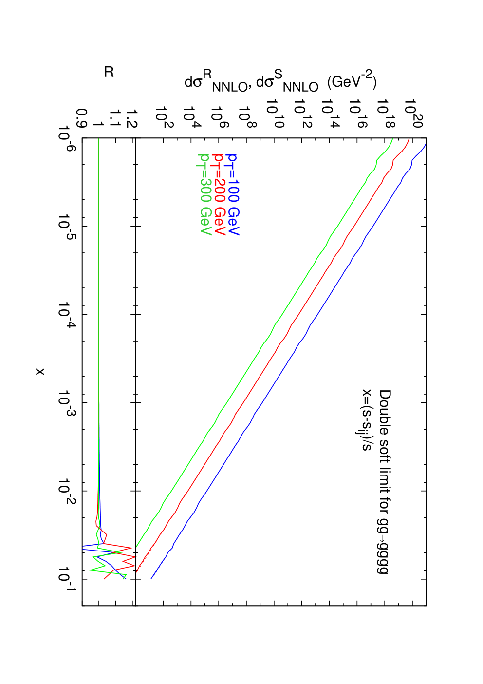
Refer to caption
Figure 12: Matrix element squared (solid lines) and the subtraction term (dashed lines) as a function of x=(s−si​j)/sx=(s-s_{ij})/s for three different values of pTp_{T} for the final state. Also plotted is R.

In figure 12 we explicitly show the behaviour of the matrix element squared and the subtraction term as a function of xx and three choices of the jet transverse energy threshold, pT>100p_{T}>100 GeV (blue), pT>200p_{T}>200 GeV (red) and pT>300p_{T}>300 GeV (green). It is clear that both d​σ^N​N​L​OR{\rm d}\hat{\sigma}^{R}_{NNLO} and d​σ^N​N​L​OS{\rm d}\hat{\sigma}^{S}_{NNLO} diverge in the double soft limit x→0x\to 0 but their ratio approaches unity.

6.2 Triple collinear limit

We now consider the triple collinear region of the phase space where three hard particles share a collinear direction. There are two separate configurations where the three collinear partons form either a final state (fig. 13(a)) or an initial state particle (fig. 14(a)).

Refer to caption

(a)

Refer to caption

(b)

Figure 13: (a) Example configuration of a triple collinear event with si​j​k→0s_{ijk}\to 0. (b) Distribution of RR for 10000 triple collinear phase space points.
Refer to caption

(a)

Refer to caption

(b)

Figure 14: (a) Example configuration of a triple collinear event with s1​j​k→0s_{1jk}\to 0. (b) Distribution of RR for 10000 triple collinear phase space points.

For the final state case, si​j​k→0s_{ijk}\to 0 and fig. 13(b) shows the distribution of RR for 10000 phase space points for three values of x=si​j​k/sx=s_{ijk}/s [x=10−7x=10^{-7} (red), x=10−8x=10^{-8} (green), x=10−9x=10^{-9} (blue)]. For x=10−9x=10^{-9} we obtained an average of R=1.0000004R=1.0000004 and a standard deviation of σ=4.2×10⁻⁵\sigma=4.2\times 10^{-5}. This shows that the subtraction term coincides with the matrix element squared in this limit. The number of points that lie outside the range of the histogram is also indicated on the plot and again systematically decreases as one approaches the singular region. In principle there may be additional azimuthal correlations in the triple collinear limit. However, we see that they do not affect the stability of the integrand.

In fig. 14(b) we perform a similar analysis for the initial state singularity. In this case x=s1​j​k/sx=s_{1jk}/s [x=−10−8x=-10^{-8} (red), x=−10−9x=-10^{-9} (green), x=−10−10x=-10^{-10} (blue)] and we have a configuration with two final state gluons collinear with the initial state gluon. The triple collinear configurations involving p2p_{2} produces identical results and are not shown. For x=−10−10x=-10^{-10} we obtained an average of R=0.99954R=0.99954 with a standard deviation of σ=0.04\sigma=0.04. Fig. 14(b) shows that this singular region is also well described by the subtraction term.

6.3 Soft and collinear limit

Refer to caption

(a)

Refer to caption

(b)

Figure 15: (a) Example configuration of a soft and collinear event with si​j​k≈s12=ss_{ijk}\approx s_{12}=s and si​j→0s_{ij}\to 0. (b) Distribution of RR for 10000 soft and collinear phase space points.
Refer to caption

(a)

Refer to caption

(b)

Figure 16: (a) Example configuration of a soft and collinear event with si​j​k≈s12≡ss_{ijk}\approx s_{12}\equiv s and s1​i→0s_{1i}\to 0. (b) Distribution of RR for 10000 soft and collinear phase space points.

To probe the soft and collinear regions of the phase space, we generate an event configuration with a soft final state gluon ll by making a triple invariant si​j​ks_{ijk} close to the full center of mass energy s12s_{12}. When the two collinear gluons are in the final state, we allow the i​j​kijk cluster to decay into three particles with the constraint that si​js_{ij} is small (shown in fig. 15(a)), while for an initial state collinear singularity, we rotate the ii, jj and kk momenta such that s1​is_{1i} is small (shown in fig. 16(a)).

In the first case we use two variables to approach this unresolved limit, x=(s−si​j​k)/sx=(s-s_{ijk})/s and y=si​j/sy=s_{ij}/s. Fig. 15(b) shows three choices of xx and yy, x=y=10−4x=y=10^{-4} (red), x=y=10−5x=y=10^{-5} (green) and x=y=10−6x=y=10^{-6} (blue). For x=y=10−6x=y=10^{-6} we obtained an average of R=0.99999993R=0.99999993 with a standard deviation of σ=0.0001\sigma=0.0001.

For the initial state singularity we define x=(s−si​j​k)/sx=(s-s_{ijk})/s and y=s1​i/sy=s_{1i}/s and fig. 16(b) shows three choices of xx and yy, x=|y|=10−5x=|y|=10^{-5} (red), green x=|y|=10−6x=|y|=10^{-6} (green) and x=|y|=10−7x=|y|=10^{-7} (blue), where we obtained an average of R=0.99999998R=0.99999998 with a standard deviation of σ=1.6×10⁻⁷\sigma=1.6\times 10^{-7}.

Figs. 15 (b) and 16 (b) show that the subtraction term successfully reproduces the real radiation matrix element in the soft-collinear regions.

6.4 Double collinear limit

Refer to caption

(a)

Refer to caption

(b)

Figure 17: (a) Example configuration of a double collinear event with si​j→0s_{ij}\to 0 and sk​l→0s_{kl}\to 0 simultaneously. (b) Distribution of RR for 10000 double collinear phase space points.
Refer to caption

(a)

Refer to caption

(b)

Figure 18: (a) Example configuration of a double collinear event with sj​k→0s_{jk}\to 0 and s1​i→0s_{1i}\to 0. (b) Distribution of RR for 10000 double collinear phase space points.
Refer to caption

(a)

Refer to caption

(b)

Figure 19: (a) Example configuration of a double collinear event with s1​i→0s_{1i}\to 0 and s2​j→0s_{2j}\to 0 simultaneously. (b) Distribution of RR for 10000 double collinear phase space points.

There are three different topologies where two pairs of particles can become collinear separately by demanding that two invariants vanish simultaneously. The double invariants pair may involve two final state pairs momenta (illustrated in fig. 17(a)), or one final state pair and one initial state pair (fig.  18(a)) or two initial state pairs shown in fig. 19(a).

In each case we generate 10000 phase space points and plot the RR distribution. In the final-final case we set x=si​j/sx=s_{ij}/s, y=sk​l/sy=s_{kl}/s and show results for x=y=10−4x=y=10^{-4} (red), x=y=10−6x=y=10^{-6} (green) and x=y=10−8x=y=10^{-8} (blue) in in fig. 17(b). For x=y=10−8x=y=10^{-8} we obtained an average of R=0.9999995R=0.9999995 with a standard deviation of σ=0.00037\sigma=0.00037.

For the initial-final configuration we set x=sj​k/sx=s_{jk}/s, y=s1​i/sy=s_{1i}/s and show the RR distribution for x=|y|=10−6x=|y|=10^{-6} (red), x=|y|=10−8x=|y|=10^{-8} (green) and x=|y|=10−10x=|y|=10^{-10} (blue) in fig. 18(b). The average value of RR obtained for x=|y|=10−10x=|y|=10^{-10} was R=1.00012R=1.00012 with a standard deviation of σ=0.018\sigma=0.018.

In the initial-initial case we set x=s1​i/sx=s_{1i}/s, y=s2​j/sy=s_{2j}/s and show the RR distribution for x=y=−10−6x=y=-10^{-6} (red), x=y=−10−8x=y=-10^{-8} (green) and x=y=−10−10x=y=-10^{-10} (blue) in fig. 19(b)). The average value of RR obtained for x=y=−10−10x=y=-10^{-10} was R=1.00001R=1.00001 with a standard deviation of σ=0.004\sigma=0.004.

In all three cases we found convergence of the matrix element and the counterterm as we approach the double collinear limits. As expected the number of outliers systematically decreases as we approach the singular region.

6.5 Subtraction of single unresolved final and initial state singularities

In this subsection we will check that the integrand defined by the matrix element with colour ordered gluonic amplitudes and subtraction term with antenna functions is integrable over the single unresolved phase space regions. Single unresolved subtraction is well understood at NLO, but, in this case it is necessary to verify that the new NNLO subtraction term does not introduce divergences when one parton becomes unresolved. In other words it has to be correct simultaneously for both double unresolved and single unresolved configurations. In the 2→42\to 4 phase space these correspond to three jet configurations and, depending on the observable, these are allowed by the jet defining function through cuts on the final state momenta.

6.5.1 Soft limit

Refer to caption

(a)

Refer to caption

(b)

Figure 20: (a) Example configuration of a single soft event with si​j​k≈s12=ss_{ijk}\approx s_{12}=s. (b) Distribution of RR for 10000 single soft phase space points.

In figure 20(a) we analyse the limit where gluon ll is soft which is described by configurations where a triple invariant si​j​ks_{ijk} is close to the full center of mass energy s=s12s=s_{12}. We defined x=(s−si​j​k)/sx=(s-s_{ijk})/s and show the distributions for x=10−5x=10^{-5} (red), x=10−6x=10^{-6} (green) and x=10−7x=10^{-7} (blue) in fig. 20(b). We see that the subtraction term converges to the matrix element as we approach the single soft limit. In this case the singularities related to soft gluons cancel and, the piece of the subtraction term described in section 4.5 correctly subtracts point by point the oversubtraction of large-angle soft gluon radiation. For x=10−7x=10^{-7} we obtained an average R=0.999998R=0.999998 and a standard deviation of σ=1.9×10⁻⁵\sigma=1.9\times 10^{-5}.

6.5.2 Collinear limit

Refer to caption

(a)

Refer to caption

(b)

Figure 21: (a) Example configuration of a single collinear event with sj​k→0s_{jk}\to 0. (b) Distribution of RR for 10000 single collinear phase space points.
Refer to caption

(a)

Refer to caption

(b)

Figure 22: (a) Example configuration of a single collinear event with s1​i→0s_{1i}\to 0. (b) Distribution of RR for 10000 single collinear phase space points.

Finally we generate points corresponding to the final and initial state single collinear regions of the phase space. These event topologies are shown in figs. 21(a) and 22(a) respectively.

For the final-final collinear singularity, we introduce the variable x=si​j/s12x=s_{ij}/s_{12} and fig. 21(b) shows the distribution for x=10−8x=10^{-8} (red), x=10−9x=10^{-9} (green) and x=10−10x=10^{-10} (blue). Similarly in the initial-final collinear limit, we define x=s1​i/s12x=s_{1i}/s_{12} and show the distributions of RR for the same xx-values in fig. 22(b).

As we have discussed in section 4.7.2, using scalar four-parton antennae functions the factorisation in the collinear limits where a final state gluon splits into two gluons introduces angular terms. This is the reason why the distributions in figs. 21(b) and 22(b) have a much broader shape than the previous examples. It is clear that as we approach the collinear limits x→0x\to 0, the azimuthal terms are not suppressed and the subtraction term is not, point by point, a better representation of the matrix element.

Nevertheless, the azimuthal terms coming from the single collinear limits were shown to vanish in sect. 4.7.2. This occurs globally after an azimuthal integration over the unresolved phase space. Here we are performing a point-by-point analysis on the integrand defined by the matrix element squared and the subtraction term. One possible strategy is to introduce the angular ΘF30​(i,j,z,k⟂)\Theta_{F_{3}^{0}}(i,j,z,k_{\perp}) function defined in sect. 4.7.2 to reconstruct the angular terms. Subtracting this additional term from the F40F_{4}^{0} four-parton antenna functions for the final-final and, initial-final and initial-initial configurations (by crossing momenta to the initial state) should produce a subtraction term that is locally free of angular terms.

Refer to caption

(a)

Refer to caption

(b)

Figure 23: Distribution of RR for 10000 single collinear phase space points for the azimuthally corrected subtraction term for (a) Final state collinear singularities with si​j→0s_{ij}\to 0 and (b) Initial state collinear singularities with s1​i→0s_{1i}\to 0.

With this azimuthally modified subtraction term, we recompute the distributions in figs. 23. In fig. 23(a) we show the RR distribution for 10000 final state single collinear phase space points and x=10−8x=10^{-8} (red), x=10−10x=10^{-10} (green) and x=10−12x=10^{-12} (blue). For x=10−12x=10^{-12} we obtained an average R=0.99994R=0.99994 and a standard deviation of σ=0.015\sigma=0.015.

We repeat the same analysis for the initial state collinear configuration in fig. 23(b) for x=−10−8x=-10^{-8} (red), in green x=−10−10x=-10^{-10} (green) and in blue x=−10−12x=-10^{-12} (blue). For x=−10−12x=-10^{-12} we obtained an average of R=1.00007R=1.00007 and a standard deviation of σ=0.012\sigma=0.012.

For both cases, the distributions now peaks around R=1R=1 with a more pronounced peak as the limit is approached, just as in the double unresolved and single soft limits discussed earlier. This demonstrates the convergence of the counterterm to the matrix element.

We note that simply introducing the azimuthal correction term ΘF30​(i,j,z,k⟂)\Theta_{F_{3}^{0}}(i,j,z,k_{\perp}) has the unfortunate side effect of generating new singularities in the previously analysed (double unresolved) phase space regions. For example, looking into equation () for ΘF30​(i,j,z,k⟂)\Theta_{F_{3}^{0}}(i,j,z,k_{\perp}) we see invariants in the denominator that are not compensated by a small quantity in the numerator in the double unresolved limit. The azimuthal correction term therefore introduces new divergences which are not present in the matrix element.

Refer to caption

(a)

Refer to caption

(b)

Figure 24: Distribution of RR for 10000 single collinear phase space point pairs where the pair of phase space points is related by an azimuthal rotation of π/2\pi/2 about the collinear direction for (a) Final state collinear singularities with si​j→0s_{ij}\to 0 and (b) Initial state collinear singularities with s1​i→0s_{1i}\to 0.

A second more successful approach is to try to cancel the angular terms by combining phase space points related to each other by a rotation of the system of unresolved partons [112, 63]. When both collinear partons are in the final state, this can be achieved by considering pairs of phase space points which are related by rotating the collinear partons by π/2\pi/2 around the resultant parton direction. This is the direction defined by pμp^{\mu} in eq. (113). Similarly, for the initial-final state collinear configurations produced when piμ→pμ+pjμp_{i}^{\mu}\to p^{\mu}+p_{j}^{\mu} for i=1,2i=1,2 and with i||ji||j and p2=0p^{2}=0, the phase space points should again be related by rotations of π/2\pi/2 about the direction of pμp^{\mu}. This has the consequence of rotating piμp_{i}^{\mu} off the beam axis and therefore has to be compensated by a Lorentz boost.

The effect of combining pairs of phase space points is shown in Fig. 24 for the same values of small parameter: |x|=10−8|x|=10^{-8} (red), 10−1010^{-10} (green) and 10−1210^{-12} (blue) for x=si​j/s12x=s_{ij}/s_{12} and x=s1​i/s12x=s_{1i}/s_{12} respectively. We see that the distributions for both final-final and initial-final collinear limits have a very sharp peak around R=1R=1. For the final state singularity and x=10−12x=10^{-12} we obtained an average of R=0.999996R=0.999996 and a standard deviation of σ=0.00015\sigma=0.00015. Similarly, for the initial state collinear singularity and x=−10−12x=-10^{-12} we found R=0.9999991R=0.9999991 and σ=0.00011\sigma=0.00011. There is an enormous improvement compared to the raw distributions shown in Figs. 21 and 22 and a significant improvement compared to adding an azimuthal correction term shown in Fig. 23. The modified subtraction term clearly converges to the matrix element as we approach the single collinear limit and correctly subtracts the azimuthally enhanced terms in a point-by-point manner.

7 Conclusions

In this paper, we have generalised the antenna subtraction method for the calculation of higher order QCD corrections to exclusive collider observables for situations with partons in the initial state to NNLO.

The basic ingredients for the antenna subtraction terms, are the antenna functions, which can be obtained from the known final-state antenna functions by simple crossing [38, 94], the momentum mappings for double unresolved configurations that have the correct behaviour in the unresolved limits [94] and the integrated form of the antenna functions [38, 94, 77, 79]. Here, we derived general subtraction terms for all NNLO processes with two hadrons in the initial state.

We focussed particular attention on the application of the antenna subtraction formalism to construct the subtraction term relevant for the gluonic double real radiation contribution to dijet production. The gluon scattering channel is expected to be the dominant contribution at NNLO, but the subtraction term also involves the four-gluon antenna function F40F_{4}^{0} which has not been encountered in previous NNLO calculations. The gluonic subtraction term includes a mixture of three-parton and four-parton antennae functions in final-final, initial-final and initial-initial configurations. The subtraction terms for processes involving quarks will make use of the same antenna building blocks and momentum mappings given discussed here but are expected to be simpler.

By construction the counterterm subtracts double and single unresolved singularities in the final and initial state. It is constructed using the analytic behaviour of the antenna in the single and double unresolved limits. We therefore tested that our implementation of the antenna subtraction behaves in the expected way by comparing the behaviour of the double radiation contribution with that of the subtraction term numerically. The agreement between the exact six-gluon contribution and the approximate subtraction term represents the first sanity check on the NNLO antenna subtraction method for gluonic processes. All of the single and double unresolved regions of phase space were analysed separately. The numerical results showed that the combination of the antennae correctly describes the infrared singularity structure of the matrix element, with the caveat of the correct handling of the azimuthal terms associated with the single collinear limit. All of the double unresolved and single soft singularities present in the matrix elements are cancelled in a point-by point manner. The single collinear terms can successfully be treated by combining phase space points related by rotations about the collinear directions.

Together with the integrated forms of the antenna functions (see Ref. [77] for the initial-final and Ref. [79] for the initial-initial configurations), the double real subtraction terms presented here provides a major step towards the NNLO evaluation of the dijet observables at hadron colliders. Future steps include;

  • (i)

    completion of the analytic integration of the initial-initial antenna.

  • (ii)

    the subtraction of infrared divergences in the gluonic mixed real-virtual correction which requires an analysis (and integration) of the one-loop three-gluon antenna function.

  • (iii)

    analytic cancellation of infrared poles between the analytically integrated antennae present in the subtraction terms and the two-loop four-gluon and one-loop five gluon matrix elements.

  • (iv)

    full parton-level Monte Carlo implementation of the finite four-, five- and six-gluon channels.

  • (v)

    the construction of similar subtraction terms, etc., for processes involving quarks.

The final goal is the construction of a numerical program to compute NNLO QCD estimates of di-jet production in hadron-hadron collisions.

Acknowledgments.
We acknowledge useful discussions with James Currie, Thomas Gehrmann and Adrian Signer. This research was supported in part by the UK Science and Technology Facilities Council and by the European Commission’s Marie-Curie Research Training Network under contract MRTN-CT-2006-035505 ‘Tools and Precision Calculations for Physics Discoveries at Colliders’. EWNG gratefully acknowledges the support of the Wolfson Foundation and the Royal Society. JP gratefully acknowledges the award of a Fundação para a Ciência e Tecnologia (FCT - Portugal) PhD studentship.

References

  • [1] E. W. N. Glover, Progress in NNLO calculations for scattering processes, Nucl. Phys. Proc. Suppl. 116 (2003) 3–7 [hep-ph/0211412].
  • [2] S. Catani and M. H. Seymour, A general algorithm for calculating jet cross sections in NLO QCD, Nucl. Phys. B485 (1997) 291–419 [hep-ph/9605323].
  • [3] S. Frixione, Z. Kunszt and A. Signer, Three jet cross-sections to next-to-leading order, Nucl. Phys. B467 (1996) 399–442 [hep-ph/9512328].
  • [4] Z. Nagy and Z. Trocsanyi, Calculation of QCD jet cross sections at next-to-leading order, Nucl. Phys. B486 (1997) 189–226 [hep-ph/9610498].
  • [5] S. Frixione, A General approach to jet cross-sections in QCD, Nucl. Phys. B507 (1997) 295–314 [hep-ph/9706545].
  • [6] G. Somogyi and Z. Trocsanyi, A new subtraction scheme for computing QCD jet cross sections at next-to-leading order accuracy, hep-ph/0609041.
  • [7] T. Gleisberg and F. Krauss, Automating dipole subtraction for QCD NLO calculations, Eur. Phys. J. C53 (2008) 501–523 [0709.2881].
  • [8] M. H. Seymour and C. Tevlin, TeVJet: A general framework for the calculation of jet observables in NLO QCD, 0803.2231.
  • [9] K. Hasegawa, S. Moch and P. Uwer, Automating dipole subtraction, Nucl. Phys. Proc. Suppl. 183 (2008) 268–273 [0807.3701].
  • [10] K. Hasegawa, S. Moch and P. Uwer, AutoDipole – Automated generation of dipole subtraction terms –, 0911.4371.
  • [11] R. Frederix, T. Gehrmann and N. Greiner, Automation of the Dipole Subtraction Method in MadGraph/MadEvent, JHEP 09 (2008) 122 [0808.2128].
  • [12] M. Czakon, C. G. Papadopoulos and M. Worek, Polarizing the Dipoles, JHEP 08 (2009) 085 [0905.0883].
  • [13] R. Frederix, S. Frixione, F. Maltoni and T. Stelzer, Automation of next-to-leading order computations in QCD: the FKS subtraction, JHEP 10 (2009) 003 [0908.4272].
  • [14] C. F. Berger et. al., An Automated Implementation of On-Shell Methods for One-Loop Amplitudes, Phys. Rev. D78 (2008) 036003 [0803.4180].
  • [15] W. T. Giele and G. Zanderighi, On the Numerical Evaluation of One-Loop Amplitudes: The Gluonic Case, JHEP 06 (2008) 038 [0805.2152].
  • [16] G. Ossola, C. G. Papadopoulos and R. Pittau, CutTools: a program implementing the OPP reduction method to compute one-loop amplitudes, JHEP 03 (2008) 042 [0711.3596].
  • [17] T. Binoth, J. P. Guillet, G. Heinrich, E. Pilon and T. Reiter, Golem95: a numerical program to calculate one-loop tensor integrals with up to six external legs, Comput. Phys. Commun. 180 (2009) 2317–2330 [0810.0992].
  • [18] E. W. N. Glover, C. Oleari and M. E. Tejeda-Yeomans, Two-loop QCD corrections to gluon-gluon scattering, Nucl. Phys. B605 (2001) 467–485 [hep-ph/0102201].
  • [19] Z. Bern, A. De Freitas and L. J. Dixon, Two-loop helicity amplitudes for gluon gluon scattering in QCD and supersymmetric Yang-Mills theory, JHEP 03 (2002) 018 [hep-ph/0201161].
  • [20] E. W. N. Glover and M. E. Tejeda-Yeomans, One-loop QCD corrections to gluon-gluon scattering at NNLO, JHEP 05 (2001) 010 [hep-ph/0104178].
  • [21] C. Anastasiou, E. W. N. Glover, C. Oleari and M. E. Tejeda-Yeomans, Two-loop QCD corrections to the scattering of massless distinct quarks, Nucl. Phys. B601 (2001) 318–340 [hep-ph/0010212].
  • [22] C. Anastasiou, E. W. N. Glover, C. Oleari and M. E. Tejeda-Yeomans, Two-loop QCD corrections to massless identical quark scattering, Nucl. Phys. B601 (2001) 341–360 [hep-ph/0011094].
  • [23] C. Anastasiou, E. W. N. Glover, C. Oleari and M. E. Tejeda-Yeomans, Two-loop QCD corrections to massless quark-gluon scattering, Nucl. Phys. B605 (2001) 486–516 [hep-ph/0101304].
  • [24] Z. Bern, A. De Freitas and L. J. Dixon, Two-loop helicity amplitudes for quark gluon scattering in QCD and gluino gluon scattering in supersymmetric Yang- Mills theory, JHEP 06 (2003) 028 [hep-ph/0304168].
  • [25] A. De Freitas and Z. Bern, Two-loop helicity amplitudes for quark-quark scattering in QCD and gluino gluino scattering in supersymmetric Yang- Mills theory, JHEP 09 (2004) 039 [hep-ph/0409007].
  • [26] S. Catani, The singular behaviour of QCD amplitudes at two-loop order, Phys. Lett. B427 (1998) 161–171 [hep-ph/9802439].
  • [27] Z. Bern, L. J. Dixon and D. A. Kosower, One loop corrections to five gluon amplitudes, Phys. Rev. Lett. 70 (1993) 2677–2680 [hep-ph/9302280].
  • [28] Z. Bern, V. Del Duca and C. R. Schmidt, The infrared behavior of one-loop gluon amplitudes at next-to-next-to-leading order, Phys. Lett. B445 (1998) 168–177 [hep-ph/9810409].
  • [29] Z. Bern, V. Del Duca, W. B. Kilgore and C. R. Schmidt, The infrared behavior of one-loop QCD amplitudes at next-to-next-to-leading order, Phys. Rev. D60 (1999) 116001 [hep-ph/9903516].
  • [30] S. Catani and M. Grazzini, The soft-gluon current at one-loop order, Nucl. Phys. B591 (2000) 435–454 [hep-ph/0007142].
  • [31] F. A. Berends and W. Giele, The Six Gluon Process as an Example of Weyl-Van Der Waerden Spinor Calculus, Nucl. Phys. B294 (1987) 700.
  • [32] M. L. Mangano, S. J. Parke and Z. Xu, Duality and Multi - Gluon Scattering, Nucl. Phys. B298 (1988) 653.
  • [33] M. L. Mangano and S. J. Parke, Multi-Parton Amplitudes in Gauge Theories, Phys. Rept. 200 (1991) 301–367 [hep-th/0509223].
  • [34] A. Gehrmann-De Ridder and E. W. N. Glover, A complete 𝒪⁡(α​αs){\cal O}(\alpha\alpha_{s}) calculation of the Photon + 1 Jet rate in e+​e−e^{+}e^{-} annihilation, Nucl. Phys. B517 (1998) 269–323 [hep-ph/9707224].
  • [35] J. M. Campbell and E. W. N. Glover, Double Unresolved Approximations to Multiparton Scattering Amplitudes, Nucl. Phys. B527 (1998) 264–288 [hep-ph/9710255].
  • [36] S. Catani and M. Grazzini, Collinear factorization and splitting functions for next- to-next-to-leading order QCD calculations, Phys. Lett. B446 (1999) 143–152 [hep-ph/9810389].
  • [37] S. Catani and M. Grazzini, Infrared factorization of tree level QCD amplitudes at the next-to-next-to-leading order and beyond, Nucl. Phys. B570 (2000) 287–325 [hep-ph/9908523].
  • [38] A. Gehrmann-De Ridder, T. Gehrmann and E. W. N. Glover, Antenna Subtraction at NNLO, JHEP 09 (2005) 056 [hep-ph/0505111].
  • [39] S. Weinzierl, Subtraction terms at NNLO, JHEP 03 (2003) 062 [hep-ph/0302180].
  • [40] S. Frixione and M. Grazzini, Subtraction at NNLO, JHEP 06 (2005) 010 [hep-ph/0411399].
  • [41] G. Somogyi, Z. Trocsanyi and V. Del Duca, Matching of singly- and doubly-unresolved limits of tree- level QCD squared matrix elements, JHEP 06 (2005) 024 [hep-ph/0502226].
  • [42] G. Somogyi, Z. Trocsanyi and V. Del Duca, A subtraction scheme for computing QCD jet cross sections at NNLO: regularization of doubly-real emissions, JHEP 01 (2007) 070 [hep-ph/0609042].
  • [43] G. Somogyi and Z. Trocsanyi, A subtraction scheme for computing QCD jet cross sections at NNLO: regularization of real-virtual emission, JHEP 01 (2007) 052 [hep-ph/0609043].
  • [44] G. Somogyi and Z. Trocsanyi, A subtraction scheme for computing QCD jet cross sections at NNLO: integrating the subtraction terms I, JHEP 08 (2008) 042 [0807.0509].
  • [45] U. Aglietti, V. Del Duca, C. Duhr, G. Somogyi and Z. Trocsanyi, Analytic integration of real-virtual counterterms in NNLO jet cross sections I, JHEP 09 (2008) 107 [0807.0514].
  • [46] G. Somogyi, Subtraction with hadronic initial states: an NNLO- compatible scheme, JHEP 05 (2009) 016 [0903.1218].
  • [47] P. Bolzoni, S.-O. Moch, G. Somogyi and Z. Trocsanyi, Analytic integration of real-virtual counterterms in NNLO jet cross sections II, JHEP 08 (2009) 079 [0905.4390].
  • [48] S. Catani and M. Grazzini, An NNLO subtraction formalism in hadron collisions and its application to Higgs boson production at the LHC, Phys. Rev. Lett. 98 (2007) 222002 [hep-ph/0703012].
  • [49] M. Grazzini, NNLO predictions for the Higgs boson signal in the H-¿WW- ¿lnu lnu and H-¿ZZ-¿4l decay channels, JHEP 02 (2008) 043 [0801.3232].
  • [50] S. Catani, L. Cieri, G. Ferrera, D. de Florian and M. Grazzini, Vector boson production at hadron colliders: a fully exclusive QCD calculation at NNLO, Phys. Rev. Lett. 103 (2009) 082001 [0903.2120].
  • [51] S. Catani, G. Ferrera and M. Grazzini, W boson production at hadron colliders: the lepton charge asymmetry in NNLO QCD, 1002.3115.
  • [52] T. Binoth and G. Heinrich, An automatized algorithm to compute infrared divergent multi-loop integrals, Nucl. Phys. B585 (2000) 741–759 [hep-ph/0004013].
  • [53] T. Binoth and G. Heinrich, Numerical evaluation of multi-loop integrals by sector decomposition, Nucl. Phys. B680 (2004) 375–388 [hep-ph/0305234].
  • [54] G. Heinrich, Sector Decomposition, Int. J. Mod. Phys. A23 (2008) 1457–1486 [0803.4177].
  • [55] G. Heinrich, A numerical method for NNLO calculations, Nucl. Phys. Proc. Suppl. 116 (2003) 368–372 [hep-ph/0211144].
  • [56] C. Anastasiou, K. Melnikov and F. Petriello, A new method for real radiation at NNLO, Phys. Rev. D69 (2004) 076010 [hep-ph/0311311].
  • [57] T. Binoth and G. Heinrich, Numerical evaluation of phase space integrals by sector decomposition, Nucl. Phys. B693 (2004) 134–148 [hep-ph/0402265].
  • [58] G. Heinrich, The sector decomposition approach to real radiation at NNLO, Nucl. Phys. Proc. Suppl. 157 (2006) 43–47 [hep-ph/0601232].
  • [59] C. Anastasiou, K. Melnikov and F. Petriello, Real radiation at NNLO: e+​e−→2e^{+}e^{-}\to 2 jets through 𝒪⁡(αs2𝐶𝐿𝑂𝑆𝐸{\cal O}(\alpha_{s}^{2}), Phys. Rev. Lett. 93 (2004) 032002 [hep-ph/0402280].
  • [60] C. Anastasiou, K. Melnikov and F. Petriello, Higgs boson production at hadron colliders: Differential cross sections through next-to-next-to-leading order, Phys. Rev. Lett. 93 (2004) 262002 [hep-ph/0409088].
  • [61] C. Anastasiou, K. Melnikov and F. Petriello, Fully differential Higgs boson production and the di- photon signal through next-to-next-to-leading order, Nucl. Phys. B724 (2005) 197–246 [hep-ph/0501130].
  • [62] K. Melnikov and F. Petriello, The WW boson production cross section at the LHC through O⁡(αs2)O(\alpha^{2}_{s}), Phys. Rev. Lett. 96 (2006) 231803 [hep-ph/0603182].
  • [63] A. Gehrmann-De Ridder, T. Gehrmann, E. W. N. Glover and G. Heinrich, Infrared structure of e+​e−→3e^{+}e^{-}\to 3 jets at NNLO, JHEP 11 (2007) 058 [0710.0346].
  • [64] A. Gehrmann-De Ridder, T. Gehrmann, E. W. N. Glover and G. Heinrich, Jet rates in electron-positron annihilation at O⁡(αs3)O(\alpha_{s}^{3}) in QCD, Phys. Rev. Lett. 100 (2008) 172001 [0802.0813].
  • [65] S. Weinzierl, NNLO corrections to 3-jet observables in electron-positron annihilation, Phys. Rev. Lett. 101 (2008) 162001 [0807.3241].
  • [66] S. Weinzierl, The infrared structure of e+​e−→3e^{+}e^{-}\to 3 jets at NNLO reloaded, JHEP 07 (2009) 009 [0904.1145].
  • [67] A. Gehrmann-De Ridder, T. Gehrmann, E. W. N. Glover and G. Heinrich, Second-order QCD corrections to the thrust distribution, Phys. Rev. Lett. 99 (2007) 132002 [0707.1285].
  • [68] A. Gehrmann-De Ridder, T. Gehrmann, E. W. N. Glover and G. Heinrich, NNLO corrections to event shapes in e+​e−e^{+}e^{-} annihilation, JHEP 12 (2007) 094 [0711.4711].
  • [69] A. Gehrmann-De Ridder, T. Gehrmann, E. W. N. Glover and G. Heinrich, NNLO moments of event shapes in e+​e−e^{+}e^{-} annihilation, JHEP 05 (2009) 106 [0903.4658].
  • [70] S. Weinzierl, Event shapes and jet rates in electron-positron annihilation at NNLO, JHEP 06 (2009) 041 [0904.1077].
  • [71] S. Weinzierl, Moments of event shapes in electron-positron annihilation at NNLO, Phys. Rev. D80 (2009) 094018 [0909.5056].
  • [72] G. Dissertori et. al., First determination of the strong coupling constant using NNLO predictions for hadronic event shapes in e+​e−e^{+}e^{-} annihilations, JHEP 02 (2008) 040 [0712.0327].
  • [73] G. Dissertori et. al., Determination of the strong coupling constant using matched NNLO+NLLA predictions for hadronic event shapes in e+e- annihilations, JHEP 08 (2009) 036 [0906.3436].
  • [74] G. Dissertori et. al., Precise determination of the strong coupling constant at NNLO in QCD from the three-jet rate in electron–positron annihilation at LEP, 0910.4283.
  • [75] JADE Collaboration, S. Bethke, S. Kluth, C. Pahl and J. Schieck, Determination of the Strong Coupling αS\alpha_{S} from hadronic Event Shapes and NNLO QCD predictions using JADE Data, Eur. Phys. J. C64 (2009) 351–360 [0810.1389].
  • [76] T. Gehrmann, M. Jaquier and G. Luisoni, Hadronization effects in event shape moments, 0911.2422.
  • [77] A. Daleo, A. Gehrmann-De Ridder, T. Gehrmann and G. Luisoni, Antenna subtraction at NNLO with hadronic initial states: initial-final configurations, JHEP 01 (2010) 118 [0912.0374].
  • [78] A. Daleo, A. Gehrmann-De Ridder, T. Gehrmann and G. Luisoni, NNLO Antenna Subtraction with One Hadronic Initial State, 1001.2397.
  • [79] R. Boughezal, A. Gehrmann-De Ridder and M. Ritzmann, NNLO antenna subtraction with two hadronic initial states, 1001.2396.
  • [80] D. Kosower, B.-H. Lee and V. P. Nair, Multi gluon scattering: A string based calculation, Phys. Lett. B201 (1988) 85.
  • [81] F. A. Berends and W. T. Giele, Multiple Soft Gluon Radiation in Parton Processes, Nucl. Phys. B313 (1989) 595.
  • [82] V. Del Duca, A. Frizzo and F. Maltoni, Factorization of tree QCD amplitudes in the high-energy limit and in the collinear limit, Nucl. Phys. B568 (2000) 211–262 [hep-ph/9909464].
  • [83] T. G. Birthwright, E. W. N. Glover, V. V. Khoze and P. Marquard, Multi-Gluon Collinear Limits from MHV diagrams, JHEP 05 (2005) 013 [hep-ph/0503063].
  • [84] T. G. Birthwright, E. W. N. Glover, V. V. Khoze and P. Marquard, Collinear Limits in QCD from MHV Rules, JHEP 07 (2005) 068 [hep-ph/0505219].
  • [85] Z. Bern, L. J. Dixon, D. C. Dunbar and D. A. Kosower, One-Loop n-Point Gauge Theory Amplitudes, Unitarity and Collinear Limits, Nucl. Phys. B425 (1994) 217–260 [hep-ph/9403226].
  • [86] D. A. Kosower, All-order collinear behavior in gauge theories, Nucl. Phys. B552 (1999) 319–336 [hep-ph/9901201].
  • [87] D. A. Kosower and P. Uwer, One-Loop Splitting Amplitudes in Gauge Theory, Nucl. Phys. B563 (1999) 477–505 [hep-ph/9903515].
  • [88] S. Catani, D. de Florian and G. Rodrigo, The triple collinear limit of one-loop QCD amplitudes, Phys. Lett. B586 (2004) 323–331 [hep-ph/0312067].
  • [89] D. A. Kosower, All-orders singular emission in gauge theories, Phys. Rev. Lett. 91 (2003) 061602 [hep-ph/0301069].
  • [90] S. Weinzierl, Subtraction terms for one-loop amplitudes with one unresolved parton, JHEP 07 (2003) 052 [hep-ph/0306248].
  • [91] Z. Bern, L. J. Dixon and D. A. Kosower, Two-Loop g→g​gg\to gg Splitting Amplitudes in QCD, JHEP 08 (2004) 012 [hep-ph/0404293].
  • [92] S. D. Badger and E. W. N. Glover, Two-loop splitting functions in QCD, JHEP 07 (2004) 040 [hep-ph/0405236].
  • [93] J. M. Campbell, M. A. Cullen and E. W. N. Glover, Four jet event shapes in electron positron annihilation, Eur. Phys. J. C9 (1999) 245–265 [hep-ph/9809429].
  • [94] A. Daleo, T. Gehrmann and D. Maitre, Antenna subtraction with hadronic initial states, JHEP 04 (2007) 016 [hep-ph/0612257].
  • [95] A. Gehrmann-De Ridder and M. Ritzmann, NLO Antenna Subtraction with Massive Fermions, JHEP 07 (2009) 041 [0904.3297].
  • [96] A. Gehrmann-De Ridder, T. Gehrmann and E. W. N. Glover, Infrared Structure of e+​e−→2e^{+}e^{-}\to 2 jets at NNLO, Nucl. Phys. B691 (2004) 195–222 [hep-ph/0403057].
  • [97] A. Gehrmann-De Ridder, T. Gehrmann and E. W. N. Glover, Quark-Gluon Antenna Functions from Neutralino Decay, Phys. Lett. B612 (2005) 36–48 [hep-ph/0501291].
  • [98] A. Gehrmann-De Ridder, T. Gehrmann and E. W. N. Glover, Gluon-Gluon Antenna Functions from Higgs Boson Decay, Phys. Lett. B612 (2005) 49–60 [hep-ph/0502110].
  • [99] D. A. Kosower, Antenna factorization of gauge-theory amplitudes, Phys. Rev. D57 (1998) 5410–5416 [hep-ph/9710213].
  • [100] D. A. Kosower, Antenna factorization in strongly-ordered limits, Phys. Rev. D71 (2005) 045016 [hep-ph/0311272].
  • [101] S. D. Ellis, Z. Kunszt and D. E. Soper, The one jet inclusive cross-section at order αs3\alpha_{s}^{3}: gluons only, Phys. Rev. Lett. 62 (1989) 726.
  • [102] S. D. Ellis, Z. Kunszt and D. E. Soper, The one jet inclusive cross-section Antenneat order αs3\alpha_{s}^{3} quarks and gluons, Phys. Rev. Lett. 64 (1990) 2121.
  • [103] S. D. Ellis, Z. Kunszt and D. E. Soper, Two jet production in hadron collisions at order αs3\alpha_{s}^{3} in QCD, Phys. Rev. Lett. 69 (1992) 1496–1499.
  • [104] W. T. Giele, E. W. N. Glover and D. A. Kosower, Higher order corrections to jet cross-sections in hadron colliders, Nucl. Phys. B403 (1993) 633–670 [hep-ph/9302225].
  • [105] W. T. Giele, E. W. N. Glover and D. A. Kosower, The Two-Jet Differential Cross Section at 𝒪⁡(αs3){\cal O}(\alpha_{s}^{3}) in Hadron Collisions, Phys. Rev. Lett. 73 (1994) 2019–2022 [hep-ph/9403347].
  • [106] R. Kleiss, W. J. Stirling and S. D. Ellis, , Comput. Phys. Commun. 40 (1986) 359.
  • [107] Z. Bern and D. A. Kosower, The Computation of loop amplitudes in gauge theories, Nucl. Phys. B379 (1992) 451–561.
  • [108] D. A. Kosower, Multiple singular emission in gauge theories, Phys. Rev. D67 (2003) 116003 [hep-ph/0212097].
  • [109] W. B. Kilgore, Subtraction terms for hadronic production processes at next-to-next-to-leading order, Phys. Rev. D70 (2004) 031501 [hep-ph/0403128].
  • [110] A. Gehrmann-De Ridder, T. Gehrmann and G. Heinrich, Four-particle phase space integrals in massless QCD, Nucl. Phys. B682 (2004) 265–288 [hep-ph/0311276].
  • [111] G. Altarelli and G. Parisi, , Nucl. Phys. B126 (1977) 298.
  • [112] S. Weinzierl, Status of jet cross sections to NNLO, Nucl. Phys. Proc. Suppl. 160 (2006) 126–130 [hep-ph/0606301].