Security Games with Decision and Observation Errors

Game theory has recently been used as an effective tool to model and solve many security problems in computer and communication networks. In a noncooperative matrix game between an Attacker and a Defender, if the payoff matrices are assumed to be known to both players, each player can compute the set of Nash equilibria of the game and play one of these strategies to maximize her expected gain (or minimize its expected loss)¹¹ 1 The problem of each player choosing a Nash equilibrium out of multiple Nash equilibria is not discussed within the scope of this paper.. However, in practice, the players do not necessarily have full knowledge of each other’s payoff function. If the game is repeated, a mechanism called fictitious play (FP) can be used for each player to learn her opponent’s motivations. In a FP process, each player observes all the actions and makes estimates of the mixed strategy of her opponent. At each stage, she updates this estimate and plays the pure strategy that is the best response (or generated based on the best response) to the current estimate of the other’s mixed strategy. It can be seen that in a FP process, if one person plays a fixed strategy (either of the pure or mixed type), the other person’s strategy will converge to the best response to this fixed strategy. Furthermore, it has been shown that, for many classes of games, such a FP process will finally render both players playing the Nash equilibrium.

In this paper, we examine a two-player game, where an Attacker (denoted as player $1$ or $P_{1}$) and a Defender (denoted as player $2$ or $P_{2}$) participate in a discrete-time repeated nonzero-sum matrix game. In a general setting, the Attacker has $m$ possible actions and the Defender has $n$ posssible actions to choose from. When such a security game is played between two automated systems over a network, in order to have a good model, we have to take into account several practical issues. First, the players may make random decision errors from time to time. Instead of playing an action $a_{i}^{j}$ that is the output of the best-response computation, player $i$ may play another action $a_{i}^{k}$ with some probability (which is typically small for functional systems). Second, the observation that each player makes on her opponent’s actions may also be incorrect, which will definitely affect her own responding actions. There are many factors giving rise to these problems: The non-idealiality of electronic and software systems, the uncertain and noisy characteristic of observation data, and the erroneous nature of the channels on which commands and observations are communicated, to name a few.

It is these scenarios that we aim to address in this paper. We examine convergence of players’ strategies in the FP process with decision and observation errors. If these strategies do converge, we quantify the new Nash equilibrium and thus estimate how these decision and observation errors affect the learning process and the equilibrium of the game.

Security games have been examined extensively in a number of papers, see for example, [1, 2, 3, 4]. The work in [5] employs the framework of Bayesian games to address the intrusion detection problem in wireless ad hoc networks. In [6], the author examines the intrusion detection problem in heterogenous networks as a nonzero-sum static game. The work in [7] addresses this problem using the framework of zero-sum stochastic games [8]. In [9], we develop a network model based on linear influence networks that allows us to take into consideration the correlation among the nodes in terms of both security assets and vulnerabilities.

Relevant literature on fictitious play can be found in [10, 11, 12, 13, 14, 15, 16]. For two-player zero-sum classical FP, the convergence proof was obtained for arbitrary numbers of actions for each player ($m\times n$) [10]. For nonzero-sum games, the proofs for two-player FP have been found for the case where one player is restricted to two actions (See [12] for classical FP and [13] for stochastic FP). In [19], we address the classical FP and stochastic FP with imperfect observations for the case where each player is restricted to two actions.

Our contributions in this paper are as follows. First, we formulate the repeated security games where players make random decision errors as a fictitious play process. We discuss the convergence of such games in the general case with arbitrary numbers of actions for each player. We then establish the convergence property for several classes of games with decision errors where both players are restricted to two actions. Second, we examine the fictitious play process where the players’ observations are imperfect and the players try to compensate for the observation errors. We again establish the convergence property for the case where both players are restricted to two actions. We point out a number of scenarios that can be considered as special cases of this result.

In Section II, we introduce some background and notation adopted from [13], [14]. The analysis for the stochastic FP with decision errors is presented in Section III. In Section IV, we address the FP with observation errors. Finally, some concluding remarks end the paper.

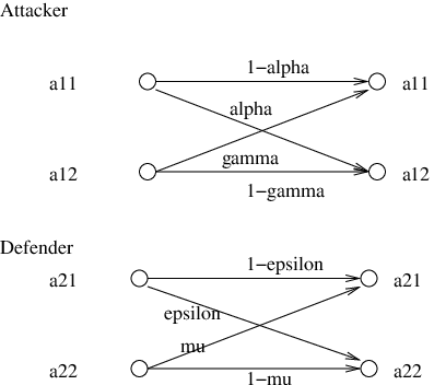
In this section, we consider the situations where players are not totally rational or the channels carrying commands are error prone. Specifically, $P_{1}$ makes decision errors with probabilities $\alpha_{ij}$’s where $\alpha_{ij},\ i,j=1\ldots m$, is the probability that $P_{1}$ intends to play action $i$ but ends up playing action $j$, $\alpha_{ij}\geq 0$, $\sum_{j=1}^{m}\alpha_{ij}=1,\ i=1\ldots m$. Similarly, $P_{2}$’s decision error probabilities are given by $\epsilon_{ij},\ \epsilon_{ij}\geq 0$, $\sum_{j=1}^{m}\epsilon_{ij}=1,\ i=1\ldots n$. This is called “trembling hand” problem in the game theory literature (See for example, Reference [17], Subsection 3.5.5). The decision error matrices $D_{1}$ and $D_{2}$ are given below.

When $m=n=2$, the decision error matrices can be written as:

The decision errors of each player in this case are illustrated in Figure 1. In what follows, we state two standard results in digital communications. The proofs are similar to those for the case $m=n=2$ in [19].

In [19], we study the effect of observation errors on convergence to the NE in a $2\times 2$ FP process. We also prove that if each player has a correct estimate of error probabilities of observations, they can reverse the effect of the channel to obtain the NE of the original static game. In this section, we present a generalized version of these results. Consider a two-player fictitious play game with imperfect observations where the error channels are given in Equations (IV) and (IV).

where $\alpha_{ij},\ i,j=1\ldots m$ is the probability that $P_{1}$’s action $i$ is erroneously observed as action $j$, $\alpha_{ij}\geq 0$, $\sum_{j=1}^{m}\alpha_{ij}=1,\ i=1\ldots m$, and $\epsilon_{ij},\ i,j=1\ldots n$ is the probability that $P_{2}$’s action $i$ is erroneously observed as action $j$, $\epsilon_{ij}\geq 0$, $\sum_{j=1}^{m}\epsilon_{ij}=1,\ i=1\ldots n$. Suppose that the players have their estimates of the errror probabilities as follows:

where $\overline{\alpha}_{ij}\geq 0$, $\sum_{j=1}^{m}\overline{\alpha}_{ij}=1,\ i=1\ldots m$, and $\overline{\epsilon}_{ij}\geq 0$, $\sum_{j=1}^{m}\overline{\epsilon}_{ij}=1,\ i=1\ldots n$.

We first restate Propositions 1 and 2 in the context of repeated games with imperfect observations.

If both players have their estimates of the errror probabilities as in Equations (IV) and (IV), they can play the stochastic FP algorithm given in II-C2 with $f_{-i}(\overline{q}_{-i})=(\overline{C}_{i})^{-1}\overline{q}_{-i}$ to compensate for observation errors (Using the results in Propositions 4 and 5). Again we can use the same procedure as in Subsection III-B to approximate the discrete-time FP with the continuous-time version.

The continuous-time approximation is given by:

It can be seen that a pair of mixed strategies $(q^{*}_{1},q^{*}_{2})$ that satisfies

will be an equilibrium point of the dynamics (60). For some results on the stability of the equilibrium point in the continuous-time system and the discrete-time system for general values of $m$ and $n$, we refer to [20]. When $m=n=2$, again the point $(p^{*}_{1},p^{*}_{2})$ is globally stable for the continuous-time system under some mild assumptions. We have the following theorem.

where $\sigma(.)$ is the soft-max function defined in (6).

In this paper, we have introduced and discussed some repeated security game models that take into account players’ decision errors and observation errors. Each player does not have access to her opponent’s payoff matrix and thus has to learn this through the fictitious play process. However, in a practical setting, each player is expected to make random decision errors from time to time and also has to respond to imperfectly observed actions of the other player. We have studied the convergence property of such games and, if the FP process does converge, quantified the new equilibrium. Such analyses will help provide guidelines for players to maximize their gain or minimize their loss in a nonideal environment.

We normally start from the mean dynamics of the discrete-time version of a game, proceed to continuous-time approximation and then analyze convergence of this continuous-time version. Although the convergence of the continuous-time fictitious play does not guarantee the almost sure convergence of the discrete-time counterpart, it does provide the necessary limiting results for the discrete-time version.

We would like to thank Deutsche Telekom Laboratories and the Boeing Company for their support. We are also grateful to the anonymous reviewers for their valuable comments.

References

- [1] T. Alpcan and T. Başar, “A Game Theoretic Approach to Decision and Analysis in Network Intrusion Detection”, Proceedings of the 42nd IEEE Conference on Decision and Control, Hawaii, USA, 2003, pp. 2595–2600.
- [2] T. Alpcan and T. Başar, “A game theoretic analysis of intrusion detection in access control systems,” Proceedings of the 43rd IEEE Conference on Decision and Control, Paradise Island, Bahamas, 2004, pp. 1568–1573.
- [3] T. Alpcan and T. Başar, “An intrusion detection game with limited observations,” Proceedings of the 12th Int. Symp. on Dynamic Games and Applications, Sophia Antipolis, France, 2006.
- [4] Z. Yin, “Trust-based game-theoretic intrusion detection,” M.S. thesis, University of Illinois at Urbana-Champaign, 2006.
- [5] Y. Liu, C. Comaniciu, and H. Man, “A Bayesian game approach for intrusion detection in wireless ad hoc networks,” Proceedings of the Workshop on Game Theory for Networks (GameNets), Pisa, Italy, 2006.
- [6] L. Chen, “On Selfish and Malicious Behaviors in Wireless Networks - A Non-cooperative Game Theoretic Approach,” Ph.D. thesis, Telecom ParisTech, 2008.
- [7] K. Sallhammar, “Stochastic Models for Combined Security and Dependability Evaluation,” Ph.D. thesis, Norwegian University of Science and Technology, 2007.
- [8] G. Owen, Game Theory, 3nd Ed., California: Academic Press, 2001.
- [9] K. C. Nguyen, T. Alpcan, and T. Başar, “Stochastic Games for Security in Networks with Interdependent Nodes,” Proc. of the International Conference on Game Theory for Networks (GameNets 2009), Istanbul, Turkey, May 13-15, 2009.
- [10] J. Robinson, “An iterative method of solving a game,” Ann. Math., vol. 54, pp. 296-301, 1951.
- [11] K. Miyasawa, “On the convergence of learning processes in a nonzero-sum two person game,” Econometrics Research Program, Princeton University, Research Momorandum No. 33, October 1961. Available at http://www.princeton.edu/ erp/ERParchives/archivepdfs/M33.pdf
- [12] U. Berger, “Fictitious play in games,” Economics Working Paper Archive at WUSTL. Available at: http://econpapers.repec.org/paper/wpawuwpga/0303009.htm
- [13] J. S. Shamma and G. Arslan, “Unified convergence proofs of continuous-time fictitious play,” IEEE Transactions on Automatic Control, Vol. 49, No.7, July 2004.
- [14] J. S. Shamma and G. Arslan, “Dynamic fictitious play, dynamic gradient play, and distributed convergence to Nash equilibria,” IEEE Transactions on Automatic Control, Vol. 50, No.3, March 2005.
- [15] A. Ozdaglar, “Lecture 11: Fictitious Play and Extensions,” Game Theory and Mechanism Design, MIT OpenCourseWare. Available at http://ocw.mit.edu/OcwWeb/Electrical-Engineering-and-Computer-Science/6-972Spring-2005/CourseHome/index.htm.
- [16] S. Mannor, J. S. Shamma, G. Arslan, “Online calibrated forecasts: Efficiency vs universality for learning in games,” Machine Learning, Special Issue on Learning and Computational Game Theory, Vol. 67, No. 1–2, pp. 77–115, May 2007.
- [17] T. Başar and G. J. Olsder, Dynamic Noncooperative Game Theory, 2nd ed. Philadelphia, PA: SIAM, 1999.
- [18] H. K. Khalil, Nonlinear systems, 2nd ed. Upper Saddle River, NJ: Prentice-Hall, 1998.
- [19] K. C. Nguyen, T. Alpcan, and T. Başar, “Security Games with Incomplete Information,” Proc. of the 2009 IEEE International Conference on Communications (ICC 2009), Dresden, Germany, June 14–18, 2009.
- [20] K. C. Nguyen, T. Alpcan, and T. Başar, “Security Games with Decision and Observation Errors,” Technical Report, UIUC, Oct. 2009. Available at http://decision.csl.uiuc.edu/˜knguyen4/research/research.html.