Generalization of the cavity method for adiabatic evolution of Gibbs states
Abstract
Mean field glassy systems have a complicated energy landscape and an enormous number of different Gibbs states. In this paper, we introduce a generalization of the cavity method in order to describe the adiabatic evolution of these glassy Gibbs states as an external parameter, such as the temperature, is tuned. We give a general derivation of the method and describe in details the solution of the resulting equations for the fully connected -spin model, the XOR-SAT problem and the anti-ferromagnetic Potts glass (or ”coloring” problem). As direct results of the states following method, we present a study of very slow Monte-Carlo annealings, the demonstration of the presence of temperature chaos in these systems, and the identification of a easy/hard transition for simulated annealing in constraint optimization problems. We also discuss the relation between our approach and the Franz-Parisi potential, as well as with the reconstruction problem on trees in computer science. A mapping between the states following method and the physics on the Nishimori line is also presented.
pacs
75.50.Lk,64.70.qd,89.70.EgIntroduction
Both in classical and quantum thermodynamics, it is often practical to discuss very slow variations of an external parameter so that the system remains at equilibrium, and such very slow changes are referred to as adiabatic [1]. When a macroscopic system is in a given phase, and if one tunes a parameter, say the temperature, very slowly then all observables, such as the energy or the magnetization in a magnet, will be given by the equilibrium equation of state.
Such considerations have to be revisited close to a phase transition where it is impossible to be truly adiabatic, and this is the subject of modern out-of-equilibrium theories. However, given a system at equilibrium in a well defined phase, it is always possible to consider the adiabatic evolution. In the low temperature phases of a ferromagnet, for instance, the evolution of the magnetization is different in the two phases (or Gibbs states) corresponding to the positive or negative magnetization. To describe this theoretically, one can force the system to be in the Gibbs state of choice (for instance by adding an external infinitesimal field, or fixing the boundary conditions) and then study the adiabatic evolution for each of these phases.
This simplicity, however, breaks when one considers glassy systems where the energy landscape is very complicated, and especially in the mean field setting where exponential number of phases (Gibbs states) exists. Adiabatic evolution of phases in mean field glassy systems is, however, a very important problem that has been considered —via some approximation or in very specific solvable cases — in a number of works [2, 3, 4, 5, 6, 7, 8, 9]. How to deal with this situation in general mean field glassy systems, how to chose a particular phase, and how to follow it adiabatically is the subject of the formalism presented in this work.
Mean-field glassy systems are important in many parts of modern science. We shall call a system a ”mean-field” one whenever a mean-field treatment is exact for this system: this is the case for all spin or particle models on fully connected lattices (such as the Curie-Weiss model of ferromagnets) or on sparse random lattices that are locally tree-like (such as the Bethe lattice). Over the last few years, studies of mean-field glassy systems brought many interesting results in physics as well as in computer science. Without being exhaustive, we can mention the development of mean field theories for structural glass formers [10, 11], for the jamming transition and amorphous packing [12], heteropolymer folding [13], or for quantum disordered materials [14] on the physics side. On the computer science side, many results have been obtain using mean field theory on optimization problems and neural network [15], and more recently random constraint satisfaction problems have witnessed a burst of new results via the application of the survey propagation algorithm and related techniques [16, 17]. The theory of error correcting codes is also closely related to glassy mean field system [18], etc.
A common denominator in all these systems is their complex energy landscape and a large number of phases (states), whose statistical features are amenable to an analytical and quantitative description via the replica and cavity methods [15, 19]. However, important and deep questions about the dynamical behavior in these systems remain largely unsolved, and many of them can be addressed by the knowledge of the slow dynamics. In order to motivate our approach, let us first discuss the basic universal features of the thermodynamic behavior of mean-field glassy models. As an external parameter, say the temperature , is tuned, a typical glassy system undergoes the following changes: At high temperature, the system is in a paramagnetic/liquid phase. Below the dynamical glass temperature , this phase shatters into exponentially many Gibbs states/phases, all well separated by extensive energetic or entropic barriers, leading to a breaking of ergodicity and to the divergence of the equilibration time [2, 20, 21]. As the temperature is further lowered, the number of states (relevant for the Boltzmann measure) may become finite and the structural entropy (or complexity) vanishes, this defines the static Kauzmann transition, , arguably similar to the one observed in real glass formers [22, 11]. This scenario is called the ”one-step replica symmetric” (1RSB) picture. In some models [23], the states will divide further into an infinite hierarchy of sub-states, a phenomenon called ”full replica symmetry breaking” (FRSB) [15, 19].

The 1RSB picture is well established in many mean field systems, and the cavity/replica method is able to compute the number, the size or the energy of the equilibrium Gibbs states. However, with the exception of few simple models [2, 3, 7, 6, 8, 9], an analytical description of the dynamics and of the way states are evolving upon adiabatic change of external parameters is missing. Let us consider a given setting where the need for adiabatic following is clear: Imagine an annealing experiment where the temperature is changed in time as . Take the thermodynamic limit first and then consider a very slow annealing . As long as we stay in the paramagnetic phase, we expect that such a slow annealing will equilibrate. The fact that the equilibration time is finite below can be actually proven [21, 24] and such annealing should be thud able to equilibrate down to the dynamical temperature after which the system get stuck in one of the many equilibrium Gibbs states. Computing the energy of the lowest configuration belonging to this state would thus give the limiting energy for a very slow annealing (and thus would give a bound to the performance of any annealing scheme). However, while the standard cavity and the replica method predict all the properties of an equilibrium state at a given temperature (equilibrium temperature), they do not tell how these properties change for this precise state when the temperature changes adiabatically to (actual temperature). A word of caution: We want to follow the state and stay in it. Hence by ”adiabatic” we mean here slow only linearly in the size of the system, corresponding to very long experimental times; an exponentially slow annealing always finds the ground state, but this is of course unfeasibly long.
The extension of the cavity method that we introduced in a recent Letter [25] precisely answered these questions by following adiabatically the evolution of any Gibbs state when an external parameter is changed (for an intuitive and pictorial description of our goals, see Fig. 1). This gives detailed quantitative information about the energy landscape and the long time dynamics. The aim of this subsequent publication is to derive the method in general, to discuss in detail the solutions of the resulting equations, and to discuss relations with some other settings (reconstruction on trees [26], Franz-Parisi potential [27, 28], Nishimori line [29]). We anticipate that the method will become part of the standard tool-box for mean field glassy systems and hence a detailed presentation is appropriate.
The paper is organized as follow: In Sec. I we give a brief reminder of the usual cavity method. In the two next section, we present our formalism for the adiabatic evolution of states from temperature higher (Sec. II) and lower (Sec. III) than the spin glass static/Kauzmann transition. We finally solve these equations and present our results for a fully connected model in Sec. IV and for diluted models on the Bethe lattice in Sec. V.
I Preliminaries
In this section, we first review the results of the standard cavity method that we shall use all along the text. The specific example for which we shall derive most of the results of this paper is the -spin model, also called the XOR-SAT problem. However, the derivation for all other models where the cavity method [19] can be used goes in the very same lines (and we will also work later on with the coloring problem). The reader familiar with the cavity method can skip this section and go directly to Sec. II.
I.1 The -spin model and XOR-SAT reminder
The -spin model is defined by its Hamiltonian
| (1) |
where are the Ising spins, are interactions between -uples of spins, is the strength of the interaction.
In what follows we will focus on two cases of the -spin model:
- •
XOR-SAT (parity check) problem: In this case all the interactions . The interactions can be both ferromagnetic and anti-ferromagnetic
(2) In the results section we mostly consider the spin glass case . The number of interactions (linear equations) is , where is the constraint density. The degree distributions of variables have to be specified here. The number of violated parity checks (constraints) is . The values of temperature for the -XOR-SAT problems are hence related to those for the -spin problem via a multiplicative factor 2, note that here and through the paper .
- •
Fully connected -spin model: The interactions exist for every possible -uple of spins, the mean and variance of are given by and .
The XOR-SAT problem was studied and solved in [30, 31, 32, 33], and its most important application are the low density parity check error correcting codes [34, 35]. The fully connected -spin model was introduced in [36, 37] and now stands at the root of the random first order theory of the glass transition [10, 38, 39].
In our examples we will mainly use the ensemble of random regular graphs, i.e. and obtain the fully connected limit by taking . The formulas are, however, written mostly for a general degree distribution (with a finite second moment). In the cavity equations we often need the excess degree distribution, that is the probability distribution of the number of excess edges given one edge is chosen, that is (denoting the average coordination number):
| (3) |
I.1.1 Liquid phase: Belief propagation equations
We now summarize in a very brief manner and without extensive derivations the known cavity equations for the XOR-SAT problem as we are going to need them for derivation of the states following method. We are trying the keep the equations in the most general form such that generalizations to other models are straightforward. The very principle of the cavity method is that we are working with tree-like graphs. Random graphs are locally a tree and we thus can work “as if” on a tree (we will eventually have to care of the boundary conditions and precise relation to random graphs later on). Solving problem on a tree can be done easily with a recursive procedure that was introduced by Bethe [40]. We will, however, use the modern language of computer science, where this is called the Belief Propagation (BP) equations.
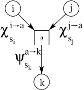
For the XOR-SAT problem the BP equations read
| (4) | |||||
| (5) |
where and are normalizations ensuring that and . The quantities (resp. ) are interpreted in terms of messages being send from a variable to a constraint (resp. from constraint to variable ) (see Fig. 2 for a pictorial representation with the so-called ”factor graph”.). Message is a probability that variable takes value conditioned on constraint to be missing from the graph. Message is a probability that the constraint is satisfied given that variable takes values . The recursion could also be written with one single type of message as
| (6) |
Given all messages computed on a given graph, one can compute the Bethe estimate of the free energy, which is also called the replica symmetric one (RS) free energy:
| (7) |
where the contributions to the free energy are
| (8) | |||||
| (9) |
Deriving the free energy with respect to the inverse temperature we get the energy
| (10) |
All the above equations are written for a given instance (graph, or given instance of the disorder) of the problem. It is often desirable to write the BP equations directly in the average form over the graph and disorder ensemble. This is the replica symmetric cavity equation
| (11) |
that can be solved numerically via the population dynamics technique introduced in [19] (see also [41] or [18] for details).
Whether the BP equations for XOR-SAT are solved on a given random graph or in the population dynamics they have always the following fixed point that corresponds to the paramagnetic/liquid phase:
| (12) |
for all and . Plugging this solution in the expression for the free energy we get
| (13) |
and for the energy we get
| (14) |
Hence in this case, the probability that a given constraint is not satisfied is
| (15) |
I.1.2 Glassy solution: One-step replica symmetry breaking
The replica symmetric liquid solution from the previous section is asymptotically exact as long as the the point-to-set correlation length stays finite [21]. This is related to the reconstruction problem on trees [26]. When the point-to-set correlation length diverges, the replica symmetry broken solution [19] has to be used to describe correctly the system.
In the one-step replica symmetry breaking one splits the phase space into exponentially many Gibbs states, is then the probability distribution over states of the cavity message . We now need to consider all these states and in order to focus on those with a given free energy , we weight them according to their Boltzmann weight to a given power , where is the so-called Parisi parameter. In the cavity method is then used as a Legendre parameter in order to select the states with a given free energy. With this in mind, the 1RSB self-consistent recursive equation reads [19]:
| (16) |
with and being defined in Eq. (6). The Parisi parameter is indeed a Legendre parameter conjugated to the internal free energy of states.The entropy associated with number of states of a given internal free energy , also called complexity and defined by , can be recovered from the following Legendre transform
| (17) |
The potential is computed from the fixed point of the 1RSB equations (16) as
| (18) |
where
| (19) | |||||
| (20) |
The condition for validity of the replica symmetric solution is recovered by solving the 1RSB equations for , that is if at there exist a non-trivial solution of Eq. (16) then RS solution is not correct and the phase space needs to be divided into states. This happens at the dynamical temperature .
The 1RSB solution is then given by the value of such that
| (21) |
Above the Kauzmann temperature one has and , that is exponentially many states are relevant to the Boltzmann measure. In this phase the local magnetization (marginal probabilities) and the thermodynamic potentials, such as the total free energy, are still given by the replica symmetric solution Eqs. (12–15).
Below the Kauzmann temperature and , the Boltzmann measure is dominated by only a finite number of states. However, an exponential numbers of sub-dominant (non-equilibrium) states still exist at any positive temperature.
I.2 Coloring of graphs, alias the anti-ferromagnet Potts model
We shall also illustrate some of our results on the anti-ferromagnetic Potts model on random graphs, mostly known and studied in its zero temperature version as then it is equivalent to the graph coloring problem [42, 43, 44, 45, 41]. The Hamiltonian is
| (22) |
where are Potts spins taking one of the possible values (colors), is the Kronecker delta symbol and the sum all edges of the graph. The phase diagram of this model at finite temperature is summarized in [46] and all the necessary equations for both the replica symmetric and glassy solution can be found in [41].
II Evolution of states above the Kauzmann temperature
In this section we introduce the states following formalism, and derive equations for the evolution of states that are at equilibrium above the Kauzmann temperature, . In this phase, the paramagnetic replica symmetric solution (12–15) correctly describes all thermodynamic quantities (but misses the ergodicity breaking at ). In the next section III we give a generalization for equilibrium states below and for meta-stable states.
In order to get an intuitive idea of what we will do, let us consider the ferromagnetic Ising model on a random graph. At low temperature, there are two phases corresponding to the positive and negative magnetization. In order to study one of these phases, a good strategy is to first recognize that the random graph is locally a tree. Then one considers a tree where all spins on the boundaries are fixed to, say, a value , then far away from the boundaries, the system will be in the phase of positive magnetization. By changing the temperature the curve can be computed. We will follow the same strategy, except that choosing the correct boundaries will be slightly more involved.
The main idea behind the equations of state following is that we pick a configuration at random among the equilibrium ones at a temperature , and then we look at the solution of the belief propagation equations at a temperature initialized in that configuration. We will also discuss a special case of factorized replica symmetric solution where this idea can be actually performed on a single graph. This is also closely related to the quiet planting discussed in [47, 48].
II.1 Gedanken experiment on infinite trees

Let us consider the problem on a large hyper-tree. Let the hyper-tree have the same distribution of disorder (i.e. the degree distribution, the distribution of negations, interaction strengths etc.) as the original problem. Let us consider a measure uniform over all configurations having energy corresponding to a given temperature . To sample uniformly one configuration from this measure the following steps need to be done:
- (a)
Take much larger hyper-tree and start with a random messages on the boundary of the larger hyper-tree and iterate the belief propagation equations at temperature down to the root. This way one created messages taken from the replica symmetric solution on the original hyper-tree.
- (b)
Assign a value to the root according to the incoming message. Proceed iteratively up to the leaves of the hyper-tree with the following: Given the value of variable choose the set of values according to probability defined in Eq. (6), where is a descendant of and for each .
Now consider the values of variables from the configuration we picked on the leaves. This is a boundary condition that defines the equilibrium Gibbs state at temperature (as long as ). Next consider the belief propagation equations at temperature , initialize the messages on the leaves of the hyper-tree in the configuration we picked (i.e. and for all if we picked value ) and iterate down to the root. The result of these iteration does describe properties (free energy, energy, size, overlap) of the Gibbs state at the temperature .
In case the original temperature was above the dynamical glass temperature, , the solution of the belief propagation at will not be different from the result of the pure BP at . That is because all the equilibrium configurations above lie in the same paramagnetic state.
When the original temperature is below the dynamical glass temperature, , the situation is much more interesting. Then the equilibrium configuration we picked lies in one of the exponentially many equilibrium Gibbs states and the belief propagation equations at a different temperature do describe adiabatic evolution of that Gibbs state.
In the next subsections we shall translate the above reasoning into the cavity equations, and describe the population dynamics technique used to solve them.
II.2 The simplest case: Factorized RS solution.
The simplest form of the equations for adiabatic evolution of states can be written when the replica symmetric solution is factorized, i.e. when the values of the messages are the same. This is the case in the XOR-SAT problem where there is a BP fixed point in which for all and the message . Furthermore, this fixed point gives an asymptotically exact results above the Kauzmann temperature .
When the RS solution is factorized the step (a) in the construction of the equilibrium configuration can be skipped and the probabilities depend only on the values of variables and the inverse temperature . In the XOR-SAT in particular we have from (6)
| (23) |
Meaning that a clause is unsatisfied with probability given by (15). These probabilities are used according to step (b) to choose an equilibrium configuration on the hyper-tree. Then belief propagation equations at a temperature are initialized on the leaves in that configuration and iterated. As usual for belief propagation equations a probability distribution of the values of messages can be written. This time one has to distinguish between messages sent to the variables which were assigned value in the equilibrium configuration, and those that were assigned . Given the probabilities to choose values of variables (23), the two probability distributions have to satisfy the following self-consistent equation
| (24) |
where is the excess degree distribution, and is defined in (6). Note the use of inverse temperature in the BP equations represented by the delta function. Given a Gibbs state that is one of the equilibrium ones at temperature , Eq. (24) encode its properties when the temperature is changed to .
The learned reader will have recognize that, when , this is nothing but the 1RSB equation [26] (at Parisi parameter ). This is actually quite normal, since when the two temperatures are equal, we are just describing the properties of a typical state, which is what the 1RSB method does. Similar equations when the temperatures are equals were thus considered in many works [41, 49, 50, 47].
To solve Eq. (24) with the population dynamics we represent by an array of values for each value of . To update one element in the array we first pick degrees from the excess degree distribution, then based on value of and Eq. (23) we pick the values . After that, for each we pick random elements in the array and based on (6) we compute a new value of and replace one element in the array . We repeat many times until (based on computation of some average quantities) the convergence is reached. It is also important to note that the initial state of the populations corresponding to the boundary conditions on the hyper-tree is
| (25) |
The internal Bethe free energy of the state is
| (26) | |||||
The value can be computed using a population dynamics procedure based on the fixed point for Eq. (24).
II.3 The case of a general (non-factorized) RS solution
In a general case when the replica solution is not factorized, e.g. in the canonical case of the random K-SAT problem, the situation is a bit more complex. In the gendanken experiment of section II.1, the uniform boundary conditions have been created with (and thus depends on) the replica symmetric marginals . The procedure described in the gedanken experiment translates to a more general form of equations, that are exact on a tree. The equivalent of eq. (24) then reads
| (27) | |||||
where is an arbitrary interaction between spins of ”strength” , in case of XOR-SAT we had . This equation is maybe easier to understand from the population dynamics procedure used to solve it. Now we have different arrays to represent the messages. In the first array we initially put an equilibrated replica symmetric population (values obtained by solving the simple RS equations by population dynamics). In the array corresponding to value we initially put a message completely polarized in the direction .
Updating one element have to be done in all the arrays simultaneously. One first chooses the degrees , then one chooses the corresponding number of random elements in the population. One uses the first array to compute the new value corresponding to the first array in the new element. To compute a new value corresponding to array one uses the values on the first array to draw a configuration of values using probabilities
| (28) |
Finally using elements in arrays corresponding to values one computes a new value. This done for every value of finalizes one step. All is repeated until convergence is reached. The expression for the free energy is analogous to (26) using the same generalization as for (27).
We note that when , the above equations are actually already known, and are exactly equivalent to the 1RSB equations at . Again, this is just because in that case, we are just describing the properties of a typical state. With equal temperatures the above form of the 1RSB equations at appeared in [51, 50, 48] (to which we refer the reader interested to see how the present derivation generalizes) and similar equations appeared in the context of the analysis of an idealized BP decimation algorithms in [52, 53].
II.4 The relation to the problem of reconstruction on trees
In the special case when the above equations are thus equivalent to the 1RSB equations when the Parisi parameter , and are closely related to the problem of reconstruction of trees, an important setting in computer science and information theory, as was first realized by Mézard and Montanari [26].
In the reconstruction on trees, a single (configuration) is spread from the root of the tree to its leaves with some given rules and noise level, and the task is then to reconstruct (infer) the value of the root based on the configuration on the leaves. In particular in a model with a factorized replica symmetric solution, constructing an equilibrium configuration on the tree has a simple local interpretation, as e.g. in [26]. The noise level corresponds to the equilibrium temperature . This spreading construction is precisely the one we have used in Fig. 3 for the XOR-SAT problem: starting from a value of the spin chosen randomly, we have chosen iteratively the configuration of the other variables randomly such that it violates the constraints with probability , corresponding to .
In the reconstructing on trees one thus applies BP starting form the leaves, using the values on the boundaries as starting conditions, to generate the marginal distributions of the variables within the tree. This is precisely what we have done, the only difference is that in the reconstruction formalism, one knows the value of that has been used in order to construct the configuration on the tree, and therefore, one used the same value in the BP equation in the recovery process.
The states following problem is thus a generalization of the reconstruction on trees, where one first generates the configuration with a value (corresponding to a temperature ) but then apply the BP equation with a different value (corresponding to a temperature ).
II.4.1 Reconstruction in a noisy channel without knowledge of the noise
The method of states following can thus be viewed as a variant of reconstruction on trees. In this interpretation the noise of the channel is described by the inverse temperature . If this value is unknown, the task of reconstructing the values will be done with an priori different temperature : The behavior of equations (24) thus describe the reconstruction problem where the noise level of the channel is not known.
Two interesting remarks can be done at this point. First, it follow from the maximum likelihood principle that the best chance to reconstruct corresponds to , and in fact, this give a direct way to recover the noise value by maximizing the free energy: On a tree, both the noise value and the marginal distribution can thus be recovered in the reconstruction process. A second point is that, as we will see from the behavior of the states following method, in some cases although reconstruction is possible at it might not be possible at some (that is when trying to reconstruct by assuming the number of mistake smaller than the actual value), which is rather counterintuitive.
II.4.2 A new bound for noisy reconstruction
A last point we shall mention is that out method provides a simple way to have new bounds on noisy reconstruction. Consider indeed a problem where we have generated the boundaries with a noise level . We now use a very simple algorithm: we simply do the BP recursion with , that is, assuming that no mistakes were done in the process. In that case, a simple bound of the reconstruction threshold can be obtained by considering a probability when the boundary condition directly imply the correct value of the root [49, 54]. A similar procedure for was called naive reconstruction in [49, 50].
In the case the equations simplify and can be cast in a set of coupled equations with two variables variables – one being the probability that the value of the root is implied in the actual value, second being the probability that the value is implied wrongly. As long as the first probability is larger than the second, which is always the case in the cases we studies, this leads to new bounds on the noisy reconstruction problem. Some of these values are given in Sec. V.3 for the XOR-SAT problem. In fact, it is simply the generalization of the naive reconstruction bound to the case of noisy channels [49, 54].
II.5 Quiet planting: How to simulate impossible to simulate models?
The construction we have described in this section is related to the notion of quiet planting, which turns out to be a powerful way to perform simulations for the mean field models, that would not be possible otherwise.
Let us first stress that the thought experiment of choosing an equilibrium configuration, that lead us to the derivation on above equations, is feasible only on trees. On a random graph we would encounter problems as soon as the long cycles would start appearing when proceeding from a node playing the role of the root. Indeed, choosing an equilibrium configuration on a given random graph below the dynamical temperature requires as far as we know an exponential time.
This difficulty, however, can be bypassed in the special cases where the replica symmetric solution is factorized and in this case the adiabatic evolution of states is realizable also on a single graph instances and this has interesting algorithmic applications: it is possible to create a graph and an equilibrated configuration at the same time. The point is that when the RS solution is factorized it is possible to create a typical random graph (from the ensemble under consideration) and a configuration that is an equilibrium configuration at temperature on that graph. This concept was called ”quiet planting” and was discussed by the authors in [47, 48].
Let us first define quiet planting in the XOR-SAT problem and then justify the above claimed properties. Planting an equilibrium configuration in XOR-SAT at a given temperature (or equivalently at a given energy) works as follows: First choose a random configuration of spins , then choose a random instance from the ensemble under consideration restricted to the fact that constraints are satisfied by the chosen configuration of spins and are not satisfied. Thus, given the configuration, choose at random ( resp.) constraints out of all the possible satisfied (unsatisfied resp.) constraints. The fraction is a function of the temperature , and it is given by Eq. (15). This way for one given clause, out of the configurations that do not satisfy that clause each will happen with probability , each satisfying configurations will appear with probability . If we condition on the value of one variable contained in the clause we obtain probabilities (23). Thus if we look on a finite neighborhood of a variable in a very large planted hyper-graph we will obtain a hyper-tree statistically identical to the one described in section II.1. Consequently, Eq. (24) and (26) are the cavity equations describing the properties of the planted graph. As typical properties of the graph follow from the solution of Eq. (24), the planted graph and the planted configuration will have the same typical properties as a random graph and an equilibrium configuration. Hence, justification of the name ”quiet” planting, i.e. planting that does not change properties of the ensemble.
Note here that the above argument was possible only because the probabilities (23) were independent of the values of messages . On the other hand, whenever this is the case, i.e. whenever the replica solution is factorized, the above argument is valid. In a general factorized case, i.e. for non-symmetric interactions or when disorder in the interactions is present, the planting procedure have to be slightly generalized. The marginal probabilities are used to plant a configuration with a proper number of each value (proper magnetization). Based on the RS solution one has to compute probabilities that a given type of constraint has given set of values on its neighboring variables and plant the constraints accordingly. An example of this general procedure at zero temperature was described in detail in [48].
It shall be noted at this point that the equivalence between the planted and purely random ensemble has been proven rigorously in [55] in the zero temperature case in the region of parameters where the second moment of the number of solutions is smaller than some constant times the square of the first moment. E.g. in the coloring problem for 3 colors the above holds till average degree , for 4 colors until , to be compared with the Kauzmann transition, also called the condensation transition, and . In the factorized models the annealed free energy, , starts to differ from the quenched one at the Kauzmann transition [41], and then the equivalence between the two ensembles breaks down.
Even before the proofs of [55] the equivalence between the planted and random ensemble for XOR-SAT for connectivities below the condensation transition was proven in [21], appendix A. In this special case the equality of the annealed and quenched free energies is directly linked to the absence of hyper-loops in the graph [21]. Authors of [21] used the equivalence between the planted and random ensembles and the fact that the planted configuration is one of the equilibrium configurations as a handy tool to ”equilibrate” their Monte-Carlo simulations even at temperature where the usual equilibration is impossible in feasible times.
The fact of generating for free an equilibrium configuration together with a typical realization of the disorder for all temperature is extremely useful, and allows to perform simulation that would be impossible otherwise: indeed for all the range of temperatures , it is unfeasible to find an equilibrium configuration as soon as is not ridiculously small. With the new method, this limitation disappears! The present authors have already used this in [47, 48], where one benefited from the fact that Monte Carlo, belief propagation and other dynamical procedures can be initialized in a truly equilibrium configuration. Later on, in section V, we will use this trick of quiet planting to confirm numerically, through Monte-Carlo simulations, the results of the states following method.
II.6 Reformulation using mapping on the Nishimori line
A last, and maybe the most striking, relation to previous works arise when one considers Gauge transformations. Let us consider, again, the -spin model. The equations for adiabatic evolution of states can be further simplified by exploiting a Gauge invariance. Indeed for any spin , the transformation
| (29) |
keeps the Hamiltonian Eq. (1) invariant. As shown in Fig. 3, this allows to transform the equilibrium spin configuration on any graph into a uniform one (all ), the disorder distribution then changes from (2) with to
| (30) |
where is given by (15). Since all , there is no need to distinguish between the and the sites. Eq. (24) reduces to the usual replica symmetric cavity equation for a problem with mixed ferromagnetic/anti-ferromagnetic interactions at temperature initialized in the uniformly positive state
| (31) |
The distribution of interactions (30) is given by the Nishimori-like [29, 56] relation between temperature and density of anti-ferromagnetic couplings , and arises because at the overlap with the equilibrium configuration, playing a role of magnetization in the Gauge transformed model, is equal to the overlap between two typical configurations from the state, a well known properties on the so-called Nishimori line (that is the line defined by the Nishimori relation in the temperature/ferromagnetic bias plane).
The Gauge invariance have thus transformed the task of following an equilibrium state in a glassy model into describing the evolution of the ferromagnetic state in a ferromagnetically biased model with the standard cavity approach. As we will derive in Sec. IV.2 adiabatic evolution of states in the fully connected -spin model for is thus equivalent to solving the -spin model with an additional effective ferromagnetic coupling (52), and one can thus readily take the solution of the -spin in the literature, e.g. [57, 56], to obtain properties of equilibrium states.
Similar mapping exist for all mean field models where the replica symmetric solution is factorized (see for instance [58] for glassy Potts models), however, the resulting model is not always very natural nor already known. For the -spin model the evolution of a glassy state being equivalent to melting of the ferromagnetic state on the Nishimori line has deep consequences for the physics of glasses, as will be discussed elsewhere [59].
III Evolution of states: General cavity equations for any temperature
In this section we introduce a method of states following that is suitable at any temperature, and where replica symmetry breaking is thus taken into account. The method is set for any general 1RSB states, at any value of the Parisi parameter and any temperature, as long as the corresponding states are stable towards further steps of replica symmetry breaking. Stability of the following equations towards RSB for different values of is interesting and will be discussed later.
III.1 Adiabatic evolution of 1RSB states
In order to understand the general equations for the adiabatic evolution of states, let us first briefly recall how are derived the cavity 1RSB equations that describe the equilibrium states. We work at inverse temperature where many states exist, each of them has a corresponding BP fixed point, i.e. a message on each link. As described in Sec. I.1.2, the 1RSB method uses the distribution of messages over all states with a given free energy . In order to select the free energy, we consider the BP recursion in every possible state, but we reweight each state according to the Boltzmann weight . This leads to Eq. (16).
One intuitive way to understand Eq. (16) is to think about the problem on a tree and consider many possible boundary conditions . In order to select boundary conditions that lead to the state of free energy we reweight at each steps with the Boltzmann weight . Eventually, for different such fixed point will describe states with different free energy . For more details on this derivation see [17, 51, 50].
In order to write the equations for the adiabatic evolution of the 1RSB states, we first need to describe the state via Eq. (16), and second we use another distribution that describes the same state at a new temperature . The equilibrium states at temperature arise if one uses the reweigthing . The probability distribution thus needs to be reweighted with the same factor in the state following method. Thus, the generalization of the 1RSB equations to the state following is a recursion on both and as follows
| (32) | |||||
The distribution is initialized as
| (33) |
where the is the solution of the usual 1RSB equations (16) describing the equilibrium state at an inverse temperature . Equation (32) then describes adiabatic evolution of this state at an inverse temperature . Note that the reweighting factor comes from the messages as the inverse temperature – again, this is the key element assuring that we are looking into the same state at a different temperature.
The internal free energy of the state at temperature is given in terms of node and link contributions, as usual in the 1RSB cavity method:
| (34) |
where
| (35) | |||||
| (36) |
And for the corresponding energy we have
| (37) |
Eqs. (32-37) are written for a given instance of the problem. It is instructive to describe how to solve them on average over the graph ensemble using the population dynamics method [19]. We need to keep a population (representing the average over graph) of couples of messages (one for , the other for ). Then the population is iterated in the exact same way as in the usual case [19], the whole population of couples is reweighted using the reweighting factor computed from the elements at inverse temperature .
III.2 When states themselves divide into states
So far we supposed that the state we are following does not exhibit an instability towards replica symmetry breaking. This assumption may break when temperature is low enough. To check for the local stability we can use a variant of any known method, see e.g. [60] or appendix C of [50]. One of the methods simplest to implement in the population dynamics is the monitoring of deviation of two replicas. For that we first need to find an equilibrated population at a temperature , then we copy this population and introduce a small noise. Further the two copies (replicas) are updated with the same random choices and the deviation of the two is monitored. If the deviation is going to zero the state is locally stable, if the deviation is growing the state is not stable towards replica symmetry breaking, that is the state has the tendency to divide into many smaller states. This second case can be treated in the following way.
If the state to be followed is not stable towards replica symmetry breaking then applying the 1RSB method within this state shall lead better result about its behavior. The following equations together with (16,32) describes the method
| (38) |
where the functional is define by Eq. (32). Said in words on every edge next to the population corresponding to Eq. (16) one would have to keep a population of populations, each corresponding to a sub-state. Each of these populations would be reweighted using the reweighting from Eq. (16). A second reweighting with Parisi parameter would have to be done on the level of populations. On top of all that in the non-factorized cases a population of these object would have to be kept to account for the average over the graph. Numerical resolution of such equations becomes involved and we let their implementation for the diluted models for future works.
IV First application: Adiabatic evolution of states in the fully connected -spin model
Now that we have presented the method for adiabatic evolution of states, let us show how does the solution of the equations behave and what can be learned about the physics of the -spin problem. We will also describe here the connection of the states following method to the Franz-Parisi potential [27, 28] and with the physics on the Nishimori line.
One of the simplest cases to which Eq. (24) can be applied is the fully connected -spin model. The static replica solution of the model is in [37]. In appendix A we show how to re-derive the replica symmetric equations for the fully connected -spin model as a limit of infinite connectivity of the cavity (belief propagation) equation (24). Here we only summarize the equations needed to explain how to obtain the solution for state following.
IV.1 The equilibrium solution of the fully connected -spin model
As discussed in details in appendix A, BP simplifies in the fully connected model where the amplitudes of all interactions are small, and become
| (39) |
where the local cavity magnetization. The replica symmetric solution can then be written in terms of the distribution of such cavity magnetization that are Gaussian because of the central limit theorem [61, 62]: we thus need only the average magnetization and the average overlap between configuration . The recursion reads:
| (40) | |||||
| (41) |
where we call the Gaussian integration. The free energy is a function of the fixed point of the above equations:
| (42) |
and for the replica symmetric energy density we have
| (43) |
The 1RSB solution with the value of Parisi parameter is obtained in a similar way, and the corresponding fixed point equations are
| (44) | |||||
| (45) | |||||
| (46) |
where
| (47) |
is a sum of two Gaussian variables, and is the Gaussian integral. The parameter is the average self-overlap and the average overlap between states. The 1RSB Parisi (replicated) free energy reads
| (48) | |||||
the free energy is derived as .
IV.2 Equations for adiabatic evolution of states for
Let us give a derivation of state following equations for the fully connected -spin model using the equivalence with the planted ensemble. We think about the fully connected model as the large connectivity version of the diluted model and used the planting procedure described in sec. II.5. We first plant an equilibrium configuration at inverse temperature , then initialize the belief propagation equations in this solution and iterate to a fixed point at another inverse temperature . When the temperature of planting is larger than the Kauzmann temperature, , then the planting can be done in a very natural way. One first takes the replica symmetric energy at and computes the corresponding fraction of interactions that are not satisfied at that energy. Then when constructing the planted graph one first chooses a random configuration, the sign of interactions is then chosen in such a way that fraction of them is unsatisfied and satisfied.
The value of in the fully connected -spin model is computed as follows. Let us assume , as this is really the case we are interested in, recall that we rescale the interactions in the fully connected model as , hence , there is total of interactions. The energy we want to achieve is given by (43), hence has to satisfy
| (49) |
Moreover as we consider only , in the -spin model this means that .
Now let us keep in mind the above planting, moreover consider that spin was planted (without loss of generality) and look back at equation (39), considering . The terms in the sum in the argument of the are independent (by the assumption of replica symmetry within the planted state) and their statistics is thus ruled by the central limit theorem. Thus our aim is to compute the mean and variance of the argument. If the interactions would not be correlated with the planted configuration the mean would be zero (remind we have ). If we satisfy every interaction with probability , there will be more satisfied interactions that unsatisfied ones. These interactions are biasing spin in the direction . The mean of the argument of the is thus
| (50) |
The planting only influences the directions of the interactions, thus in the variance computation nothing changes and we have again
| (51) |
Thus parameters , and are ruled again by equations (40-41) with inverse temperature and effective coupling
| (52) |
Parameter now measures how far from the equilibrium planted configuration is a typical configuration at . Also the free energy equation (42) applies to this case with inverse temperature and effective given by (52). The free energy here is, however, free energy of the planted state and thus the complexity, defined by (17) with , can be computed considering the difference
| (53) |
Consequently all the physics of adiabatic evolution of states above the Kauzmann temperature for the model can be induced from the known phase diagram of the model and Eq. (52) is the Nishimori line condition [29, 56] for the fully connected -spin model with a nonzero : This illustrates the general equivalence we have discussed in Sec. II.6 between the states following method and the original model on the Nishimori line.
The dynamical temperature can be interpreted as the spinodal point of the planted state, thus at we start to have a nontrivial solution if . And at the complexity (53) becomes negative at . Iterating Eqs. (40-41) we indeed obtain values of the two critical temperatures as known from the 1RSB solution of the -spin model. For we have and .
In the case of fully connected -spin model the state following when they start to be unstable (divide into sub-states), described in generality in Sec. III.2, can be done easily (at least on the 1RSB level) by using the mapping on a model with effective ferromagnetic coupling. Again, for the model with the 1RSB solution inside a state is equivalent to the standard 1RSB solution in a model with , Eqs. (44-46).
IV.3 Equations for adiabatic evolution of states for
We now want to follow states below the Kauzmann temperature, or metastable states above (i.e. at a Parisi parameter ). As far as we know there is no ”planting” interpretation for this case, the mapping into ferromagnetically biased model on the Nishimori line does not work either in this case. The underlying equilibrium measure at become more complicated, the derivation then must follow by rewriting equations (16,32) in the large connectivity limit.
For simplification we note that in the -spin model with we have thus the only non-trivial parameter describing the 1RSB state we aim to follow is , given by the equation (45), this summarizes Eq. (16).
To rewrite Eq. (32) we need to introduce overlap and a correlation between the two populations
| (54) | |||||
| (55) |
In appendix A.3 we remind the derivation of the standard 1RSB equations for the fully connected -spin model. What we nee here goes in a very similar manner. We define
| (56) |
and obtain similarly as in appendix A.3
| (57) | |||||
| (58) | |||||
| (59) |
The final self-consistent equations for and are then
| (60) | |||||
| (61) |
where
| (62) | |||||
| (63) |
The free energy of the followed state can be obtained by plugging expressions (92) and (84) into (35-36) and getting
| (64) |
The energy is then obtained by deriving . Again, these equation are similar to standard replica equation with a kind ferromagnetic bias, but do not have as simple form as was given by the mapping on Nishimori line for .
IV.4 What happens when one follows states: Turning cartoons into data
So far we were describing ideas and the formalism for the method of adiabatic following of Gibbs states. In the remaining subsections we describe and discuss results which can be obtained about the energy landscape and the structure of states for the fully connected -spin model, based on the previously derived equations.
One obvious application of the states following method is to compute how does the energy of equilibrium states evolve with temperature. Such energy-temperature diagrams (volume or entropy is sometimes plotted on the -axes, or density is plotted as a function of the pressure) appear in many works about glassy systems [20], for recent examples see [63, 64]. Except for a few very simplistic models such as the spherical -spin models [2, 3, 7], the random energy or random entropy model [6] or the random subcube model [9] (where the dynamics is exactly solvable), all these diagrams were drawn as qualitative schemes, or as results of Monte-Carlo simulations. Moreover, in the field of glassy dynamics, the energy landscape is often cartooned by drawing many valleys of different sizes and depths. The states following method allows to draw the above mentioned figures with actual quantitative data for any model solvable via the cavity or replica method.


The left part of Fig. 4 shows how does the energy of states depend on the temperature . The blue line is the equilibrium energy of the system at a given temperature. This curve is divided into four parts, the part above the dynamical temperature represents a high temperature liquid phase. Between the dynamical and Kauzmann temperature is the dynamical glass phase, where the free energy or energy are still given by the liquid result, but the equilibrium state is divided into exponentially many Gibbs states. Below the Kauzmann temperature the static line is obtained by solving the 1RSB equations (44-48), at this point its derivative changes discontinuously. This 1RSB solution becomes unstable below the Gardner temperature [23, 60] below which the line is dashed, as it is no longer exact, the correct FRSB energy would be higher.
Each of the red lines (five roughly parallel lines crossing the figure) is obtained by following the evolution of one of the exponentially many states equilibrium at some . When the state is heated the energy grows up to a spinodal point where the state disappears, i.e. when the only solution of equations (40-41) with given by (52) has . As approaches the spinodal point is at lower and lower temperatures, states very near to are lost almost immediately when heated. This is an interesting result as in the spherical models, the state at could be heated to much larger temperature: that is an unphysical property of the spherical model that disappears in the Ising model we have considered here.
When the state is cooled down, the energy is decreasing, but slower than the equilibrium energy. As soon as the temperature changes the state goes out of equilibrium: this corresponds to the notion of glassy states trapping the dynamics up in the energy landscape. In Fig. 4 left we plotted the energy of states supposing they are stable against replica symmetry breaking. We found, however, that this was not always the case and thus denoted the unstable, thus unphysical, part of the curves by dashing. Indeed, the dashed part of the lowest state curve even crosses the equilibrium line, which is unphysical, a clear sign that the replica symmetry is broken. The left ends of the red lines (five roughly parallel lines) correspond to another spinodal point, in the sense that the non-trivial, , solution of the RS state following equations (40-41) ceases to exist. This spinodal point does, however, not have a physical interpretation, as the states are unstable towards RSB in that region. We will see in Sec. IV.6 that this unphysical spinodal is related to a known problem in the spin-glass with ferromagnetic bias.
The right hand side of Fig. 4 depicts the same quantities as the left hand side, the difference is that for the adiabatic evolution of states we used the 1RSB equations (44-48). The part where this changes the result is distinguished by dashing. We checked that even the 1RSB description of the states is not stable towards more step of RSB, so that the exact description of the dashed parts requires a full RSB solution. The 1RSB result, however, gives a much better —and physical— approximation of the correct behavior. Still, for the upper states a non-physical spinodal point remains; this can be seen on the highest red curve when its dashed part finishes and turns into dotted green, we will describe in Sec. IV.7.2 how the green dotted line was obtained. Obtaining the FRSB is only a technical problem of solving the corresponding equations as the mapping to the partly ferromagnetic model (52) is valid on any level of RSB.
Note that our results correspond well to the solution of the dynamical equations in the spherical approximation, where indeed the transition towards more steps of replica symmetry breaking was observed [3, 7]: we expect actually this behavior to be quite universal and to be observed in any spin glass model with an 1RSB equilibrium solution.
One comment is in order here. The reader familiar with the phenomenology of the -spin model will certainly find many similarities between our results and the one advocated in [65]. In that work, the authors considered like us the states that are at higher free energies than the equilibrium ones for a given temperature , and found that at high energies these states are always unstable towards FRSB, just as we see in Fig. IV.7.2. There is, however, a major difference between our works: in [65] the authors were looking at the typical excited states at a given free energy and temperature , that is, at the most numerous ones. In our present work we instead concentrate on following the states that were typical at a given temperature. The point is that as soon as the temperature is changed, these states become out of equilibrium and not typical. If one wants to focus on the states that are the most important ones for the free energy landscape, it is necessary to consider their basins of attraction, as we do, and this is why we have developed the following state method in the first place. We will come back on this point when we will discuss the iso-complexity problem in Sec. V.3.

Fig. 5 presents the same data as Fig. 4 in a different perspective. It is a sort of direct look at the shape of states in the energy landscape. The -axis is still the energy, the -axis depicts the size (entropy) of the state. More precisely we plot a line at and . The blue (most outer) line is the entropy of the equilibrium (static) solution. The four red lines correspond to different Gibbs states. The horizontal dashed lines depict energy at which these states are the equilibrium Gibbs states. Note that according to the laws of thermodynamics the derivative of the energy at the minima have to be zero, whereas figure 5 shows a slight non-physical cusp. This is dues to the 1RSB approximation that underestimates the entropy, the FRSB solution would have the correct derivative.
IV.5 Below the Kauzmann transition: Level crossings and temperature chaos


We now turn to the description of static spin glass phase, . Fig. 6 uses equations derived in Sec. IV.3 and depicts the evolution of states that are at equilibrium below . Fig. 6 left gives the energy as a function of temperature for three states that are at equilibrium (marked by red points) at some temperature . In Fig. 6 right, we plot the free energy as a function of temperature of these states, the lower envelope of the free energies of all the states is then the equilibrium free energy. In order to enhance the differences, in the inset, we subtracted the equilibrium free energy from the free energies of the three states.
These plots clearly show that, although a finite number of states dominates the partition sum (which is the very definition of the glass phase below ), these states become out-of equilibrium as soon as the temperature is slightly changed. Even though for all the partition sum is dominated by a finite number of state: these states change entirely when the temperature is slightly modified. This is the phenomenon of temperature chaos that appears due to free energy levels crossing.
Temperature chaos has been discussed extensively in spin glasses, see for instance [66, 67, 68, 69, 70], it is crucial in the interpretation of memory and rejuvenation experiments [71, 72]. It existence was subject of debates, as its absence was advocated in many papers [73, 74, 75], as well as its presence [76, 77, 78, 79]. Our results allow to finally clearly demonstrate that temperature chaos is present in the Ising fully-connected -spins, and that it arises through many level crossings, as advocated in [6, 8].
IV.6 The phase diagram of evolving states and the mapping to a ferromagnetic -spin model


As we derived in Secs. II.6 and IV.2, all the physics of the adiabatic evolution of equilibrium states above the Kauzmann temperature for the -spin model can be induced from the known, see e.g. [57, 56], phase diagram of the -spin model. We will now discuss the phase diagram in the context of results given in Figs. 4 and 5. Fig. 7 shows two drawings of the phase diagram, the -axes in both is the actual temperature. The -axes on the left is the standard ferromagnetic bias , on the right the -axes is the equilibrium temperature (in both figures we took ). The red (dashed) line in both parts is , on the left this is the Nishimori line, on the right this is the equilibrium line. The task is to follow states that are the equilibrium ones on this line for . The horizontal black lines depict the location of the dynamical, Kauzmann and Gardner temperatures for .
The phase diagram of the -spin model with a ferromagnetic bias , Fig. 7 left hand side, see also [57, 56] has five thermodynamic phases separated by thick lines in the figure: The paramagnetic phase at high temperature (PARA). The 1RSB spin glass phase for low enough bias and that becomes a full RSB phase for . The ferromagnetic phase (FERRO) for large enough and that becomes a mixed phase with both ferromagnetic and full RSB order (MIXED) for . At low enough the system is a spin glass with an ergodicity breaking transition at and then the Kauzmann and Gardner phase transitions at and . At larger , the system undergoes a first-order ferromagnetic transition at . The ferromagnetic state is thermodynamically stable starting from the spinodal temperature , at it becomes thermodynamically dominant. Below the pink line, , the replica symmetric solution describing the ferromagnetic state ceases to be stable toward RSB and the system transits into the FRSB mixed phase. The mixed phase have some unphysical spinodals: below the light-blue line there is no non-trivial ferromagnetic RS solution. This is cured by the 1RSB approach, but only down to the green line, below which there is no non-trivial ferromagnetic 1RSB solution. The correct spinodal should be a vertical line in the FRSB computation. The Nishimori line is the red dashed curve: notice how it crosses the ferromagnetic transition exactly when and the spinodal at .
The right hand side of Fig. 7 depicts the same diagram as a function of the equilibrium temperature . Following a state at equilibrium at temperature to temperature is equivalent to looking to the ferromagnetic state on the Nishimori line at , and then to move vertically to other temperatures . The vertical strip of temperatures is hence particularly relevant for state following. The blue spinodal ferromagnetic line thus corresponds to the high temperature spinodal line in state following (see Fig. 4). The pink line to the point where the state divides into many sub-states and develops a (presumably) full replica symmetry breaking. However, we are unable to follow the state with the RS formalism below the light blue line that correspond to an unphysical spinodal. This is cured in part by the 1RSB formalism, but the same problems arises in this case below the green line, so that a FRSB solution is eventually needed to describe the adiabatic evolution of states at .
For () the phase diagram shows a ferromagnetic phase which would correspond to following a state that almost surely does not exist for a typical instance of the problem. To follow states equilibrium below the mapping to a model with a ferromagnetic bias breaks.
Two comments are in order about the spinodal and the ferromagnetic transition. Let us first discuss the spinodal, which we believe to be vertical bellow : the FRSB ferromagnetic solution in the mixed phase must exist up to the vertical blue line. However, different levels of replica symmetry breaking have different unphysical spinodal lines beyond which no-nontrivial ferromagnetic solution exist at the RSB level (the blue spinodal for RS and green for 1RSB are depicted). Such behavior is not unheard of: the very same phenomena takes place in the study of the Sherrington Kirkpatrick model in external magnetic field [80] (that is, for ). There also the boundary of the mixed is a vertical line in the FRSB solution, but differs at all finite levels of RSB [81, 15]. Similar features were observed in the dilute mean field spin glasses as well [82, 83]. In the state following method the lack of a ferromagnetic solution near to the true FRSB spinodal translates into difficulty of obtaining a sensible 1RSB upper bound on the low temperature adiabatic evolution of states with .
Let us now consider the ferromagnetic transition line bellow the Nishimori line. Nishimori proved [56] that the line was either vertical, or bending towards the ferromagnetic phase, this is also apparent from the states-following interpretation. Although it might not be completely visible from Fig. 7 (left), the analysis of the 1RSB equations shows that the line is bending slightly towards lager as is lowered, although the effect is very small (to the best of our knowledge, this was an unknown feature of this phase diagram). Interestingly, this has a clear interpretation in the states-following formalism. At zero temperature, the energy of the ferromagnetic state at is equal to the bottom energy of the equilibrium state at . As discussed in Sec. IV.5 chaos and level crossings make these states to have a larger energy than the true equilibrium one at ; as a consequence, the ferromagnetic state at and must have bottom-energy larger than the ground state energy of the system, so that the ferromagnetic transition can only happen for larger values of . Interestingly chaos disappears in the large limit (as well as in the spherical approximation) and this is why this line is strictly straight in the phase diagram of the random energy model [36], and in the spherical -spin model [84]11 1 Note that there have been a considerable amount of efforts to discover this effect in finite-dimensional spin glass, see for instance [105], and it is therefore interesting to observe it in mean field models as well..
IV.7 Relation to the Franz-Parisi potential
The idea of exploring one of the many phases in glassy mean field systems is a very natural one, and is therefore not new. Our states following approach is actually related to the one pioneered by Franz and Parisi years ago [85, 28, 3, 86], which is now commonly referred to as the Franz-Parisi potential. Their idea was to study glassy systems in presence of an attractive coupling among two real replicas, one of which being at equilibrium. Looking to the free energy of the copy when its overlap with an equilibrium configuration is tuned allows to compute the local free energy potential around this equilibrium point.
What the states following method is actually doing is to focus directly on the minimum of the Parisi-Franz potential, thus bypassing the need of an attractive couplings and making the formalism much simpler and applicable easily to the models on sparse graphs. The Franz-Parisi potential can, however, be obtained within the states following method if we fix the overlap between the state at temperature and . The purpose of the present paragraph is to explain how to do this in the -spin model. The reason is two-folds: (a) we want to make the correspondence with the Franz-Parisi formalism and (b) looking at these free energies turns out to be extremely instructive to understand the unphysical spinodal points and related issues discussed in the previous section.
Conveniently enough, in our mapping to a model with an effective ferromagnetic coupling , the ”magnetization” parameter (40) is nothing else than the overlap of the configuration under study and the planted one. This demonstrates the usefulness of the above mapping: The free energy at fixed magnetization of a -spin model with a ferromagnetic bias at the temperature is equal to the Franz-Parisi potential for the spin glass problem with temperature and .
Fixing the magnetization, i.e. ensuring , is done by introducing a Lagrange multiplier and writing the partition function of the system with a fixed magnetization as , where is a partition function of the model with an external magnetic field, i.e., with Hamiltonian . Once we compute the free energy of the model with external magnetic field the free energy of the system with magnetization fixed to is recovered via . To fix a value we need to ensure that ; the is thus a Legendre transform of .
This allows us to derive easily the Franz-Parisi potential in the -spin model. Actually, it also allows to obtain instantaneously all the (not straightforward) Franz-Parisi computations in the spherical and mixed spherical -spin models just by looking to the equilibrium free energy of the model with a ferromagnetic bias. The reader is invited for instance to compare the free energy in [84] with the Franz-Parisi potential in [3, 86].
IV.7.1 Franz-Parisi potential at the replica symmetric level
At the RS level, the equations for the -spin model with an external field become:
| (65) | |||||
| (66) |
with . The free energy is given by (42) with added in the argument of the .
Note that when the free energy is non-convex (as it is in the present case), one has to be extremely careful in solving these equations. Indeed if one simply chooses once and for all and simply performs a recursion of Eqs. (65-66) some values of will never be obtained. A good method is to first choose the desired value , and then to fix the magnetic field at each iteration such that Eq. (65) is satisfied. This can be easily generalized in the 1RSB equation. In Fig. 8, we show the results of this procedure.


The left side of Fig. 8 shows the free energy of configuration at a distance from the planted one in the ferromagnetically biased model; this is the Franz-Parisi potential. One sees that for there is no minimum except the trivial one at ; for , however, a second minimum appears, with a finite value of the overlap: this is precisely the one found in the states following approach, which is only performing a gradient descent in this free energy starting from the point , thus directly focusing on the non trivial-minima of the free energy potential.
The right hand side of Fig. 8 shows the free energy potential of configuration at a distance from the planted one when the temperature is different from the planted temperature. We have used and we can see how the free energy of the state changes with temperature. This is actually very instructive. When rising the temperature the bottom free energy of the state decreases (as a free energy should with temperature because of the positivity of entropy) while the overlap at the minimum get smaller: this is the sign that the state become larger. At even larger temperature, a spinodal point is met and the minimum (as well as the state) stop to exist.
When decreasing the temperature, we expect that both the free energy and increase, as the state gets smaller and deeper in the free energy landscape. This is indeed the case initially, but for low temperature (here ) we start to observe a non-monotonous behavior for . If the temperature is further lowered (here ) the minimum disappears, as we have seen in the previous chapter. These are non-physical features that show that the replica symmetric assumption is incorrect and that we need to break the replica symmetry.
IV.7.2 Franz-Parisi potential at the replica symmetry broken level


To obtain the 1RSB approximation of the Franz-Parisi potential we need to fix the parameter in the 1RSB equations using again an auxiliary magnetic field . The result for and is shown in Fig. 9 left. The lower line (red) is the replica symmetric result, the upper line (blue) is the 1RSB result. The two curves differ in the RS unstable zone on the left side of the plot. Unlike the unstable RS result, the 1RSB Franz-Parisi potential has a secondary physical minimum at about . Moreover, as general in replica theory, the 1RSB free energy is always larger than the RS one.
Right part of Fig. 9 shows the dependence of the magnetization at the minimum as a function of temperature . Following states becomes studying ferromagnetically biased model, in ferromagnets magnetization usually grows as the temperature decreases. Hence, the part where increases (or does not exist) is unphysical and will decrease in the FRSB solution. We can see that the physical region extends into lower temperatures for the 1RSB result. We also observed that the 1RSB magnetization is systematically larger than the RS one.
The above findings suggest a method how to obtain a lower bound on the energy of the state even at temperatures where the 1RSB solution does not exist (the 1RSB Franz-Parisi potential does not develop the secondary minima). At such temperature the magnetization at the real minima (which we would observe in the FRSB result) have to be larger than the maxima of magnetization in the 1RSB result over all . As the FRSB free energy is larger that the 1RSB one the free energy at that minima have to be larger than the 1RSB free energy at . Using this receipt we can thus obtain a lower bound on the free energy (and energy) which is probably not far from the true result. This is how we obtained the green dotted part in Fig. 4.
Note, however, that the above described construction of the lower bound is not very elegant and requires the calculation of the full Franz-Parisi potential . It is interesting to see if better approximation to the FRSB result can be obtained using different techniques.
V Second application: Energy landscape in constraint satisfaction problems and diluted models
We have discussed at length the various aspects of adiabatic evolution of Gibbs states for the simple case of fully connected -spin model because many of those aspects repeat for the computationally more involved models on sparse random graph like XOR-SAT or graph coloring. In this section we present results for those two models.
V.1 Following states in diluted spin models


In Fig. 10 we plot the energy of states versus temperature for the 3-XOR-SAT problem with degree of variables (left), (right). The behavior is extremely similar to the one of the fully connected model and the very same feature are observed: the spinodal upon heating, the transition towards symmetry breaking upon cooling, and the unphysical spinodal. Note that these plots have been obtain with the RS procedure and a first remark is that the RS computation gives a more complete results than in the fully-connected case. Since equilibrium states do not develop the Gardner instability, it is not surprising that the instability towards RSB is less strong in the out-of-equilibrium states as well. However, we observed once again that the states at equilibrium close to undergo a FRSB transition and decompose into many marginally stable sub-states: this seems to be an universal features of spin-glasses.
In order to check these results, we have performed the following numerical simulation. We have first prepared two large XOR-SAT system with and and spins at equilibrium for temperature and . Of course, since these temperatures are below the dynamic transition, this would be an impossible task if we could not use the planting trick described in Sec. II.5 that allows to prepare at virtually no computational cost a random instance together with an equilibrated configuration. Then, we have used a metropolis Monte-Carlo algorithm initialized in the planted configuration to follow the state upon slow cooling and slow heating. As shown in Fig. 11, the results of the simulation agree perfectly with the theoretical predictions, including the location of the high temperature spinodals.

As already pointed out computing the limiting energy of adiabatic simulated annealing corresponds to the zero temperature energy of a typical state with , and this requires to consider replica symmetry breaking within the states. At least the 1RSB computation plus the analysis suggested in Sec. IV.7.2 is needed to compute lower bounds on the energy achieved by the infinitely slow annealing. This is numerically involved and we will thus address it in subsequent works. Another way of accessing this energy-value would be to solve the dynamical equations [87, 88, 89, 20], which at current time seems to be even much harder task. Despite these limitations, a very useful new insight about the energy landscape and limitations of simulated annealing and other stochastic local search algorithms can be obtained from the results that we already have from the states following method, as we explain in the next section.

V.2 Canyon versus valleys
Let us turn our attention to Fig. 12. It depicts in the same manner as before the evolution of states for the 4-coloring of 9-regular random graphs. Unlike in the examples in Fig. 10 we see that all depicted states fall very fast down to zero energy. Again due to RSB instabilities, so far, we are not able to show explicitly that the state with goes down to zero energy. But in any case we see that the asymptotic behavior at zero temperature is rather different.
In order to be precise, we now distinguish between two types of states:
- •
Canyons are states with bottoms at the ground state energy.
- •
Valleys are states with bottoms strictly above the ground state energy.
By definition there is at least on canyon-state in every system. The definition is rather intuitive when looking to the carton of the energy landscape in Fig. 1. The difference between canyons and valleys is accentuated in Fig. 13 where data from Figs. 10 and 12 are plotted in order to visualize the shape of the states. The energy is plotted against the entropy for different equilibrium states. We plotted and such that the width corresponds to the logarithm of the number of configurations at energy for the Gibbs state. The left hand size is for the 3-XOR-SAT, right hand side for 4-coloring of 9-regular random graphs. The blue (the most outer) curve corresponds to the equilibrium energy and entropy. The different red curves are shapes of states equilibrium at energy depicted by the horizontal black dashed lines. The bottoms of depicted states on the left are at positive energy hence these states are valleys, whereas the bottom of the state depicted on the right is at zero energy, this is hence a canyon.


Based on the distinction between canyon-states and valley-states, we now describe two distinct types of energy landscape, depending on the basin of attraction of states at the dynamical transition :
- •
In the canyons-dominated landscape, a typical equilibrium state at is a canyon.
- •
In the valleys-dominated landscape those states are valleys.
In the previous examples, the cases of the XORSAT problem we showed have valleys dominated landscape and the coloring example is canyons dominated. This has a deep algorithmic consequence: an adiabatically slow simulated annealing is able to find the ground state in the canyons-dominated landscape, but this is not the case for the valleys-dominated landscape. In constraint satisfaction problems where one can change continuously the connectivity, we thus expect that there will be a sharp transition from the canyons-dominated landscape to the valleys-dominated landscape as the density of constraints is increased. This phase transition must happen between the clustering and satisfiability threshold, . We will now argue that the canyons/valleys transition is upper bounded by the rigidity transition introduced in [41, 49].
V.3 The warning propagation limit and the bottoms of states
It is possible to derive analytical equations for the energy of the bottoms of equilibrium states, i.e. in the zero temperature limit, . This is simply the limit of Eq. (24) that takes a simpler closed form when . Here we present these equations and their derivation for the XOR-SAT problem. We also derived corresponding equations for the graph coloring.
We consider for simplicity that degree of every variable in the XOR-SAT problem is fixed to and all interactions are antiferromagnetic . For our purpose it is convenient to rewrite Eq. (24) in terms of probability that a constraint is violated in the planted configuration, Eq. (15).
| (67) |
where the sums in the Kronecker deltas are modulo 2, and is defined by the BP equation (6) at zero temperature . In this limit we can write the warning propagation version of Eq. (67) which can be solved without the use of population dynamics.
Let us introduce the following probabilities
- •
is a probability that a given constraint is forcing variable into a value in which it was planted (warning from to )
- •
is a probability that a given constraint is forcing variable into a value in which it was not planted (warning from to )
- •
is a probability that a variable is being forced into a value into which it was planted (warning from to )
- •
is a probability that a variable is being forced into a value into which it was not planted (warning from to )
The following equations are then linking the above probabilities
| (68) | |||||
| (69) |
and
| (70) | |||||
| (71) |
Sanity check is that the above equations give and when , this is the equation for appearance of the hard fields derived in [49].
The corresponding energy is expressed as
| (72) |
where is the probability that contradictions happened when a variable and all its neighbors are added. And is the probability that a contradiction happened when the constraint was added. We have
| (73) | |||||
| (74) | |||||


The solution of these equations is depicted in Fig. 14 by a black line. Because of the relaxation within the state, the bottom is significantly lower than the equilibrium energy (red line).
Let us compare the state following result with an interesting heuristic idea to estimates the bottoms of states that was developed in [5] (see also [3]). It uses an approach called iso-complexity. Instead of exactly following the states, the authors proposed instead to count the number of states at a given temperature , and then to consider the energies at for which the number of state is equal to the one at . Iso-complexity leads, however, only to a lower bound, because ending up at lower energies would be exponentially unprobable. We see in Fig. 14 that indeed the true bottom is always at larger energy than given by the iso-complexity computation of [5].
Note also that above certain temperature the equations do not have any non-trivial solution, this corresponds again to the to the non-physical spinodal point is observed in Fig. 10. The physical reason for this is that the states are unstable against RSB and that we should have used the RSB formalism. The noise level corresponding to this spinodal point is summarized in Table 1.
| 3 | 3 | 0.01665(1) | 0.088265 | 0.571804 |
| 3 | 4 | 0.05184(1) | 0.094346 | 0.886841 |
| 3 | 5 | 0.09558(1) | 0.128800 | 0.723037 |
| 4 | 3 | 0.00656(1) | 0.011682 | 0.907334 |
| 4 | 4 | 0.03179(1) | 0.059680 | 0.933018 |
| 4 | 5 | 0.06673(1) | 0.087771 | 0.794195 |
| 4 | 6 | 0.08815(1) | 0.123228 | 0.857183 |
| 5 | 3 | 0.00349(1) | 0.006069 | 0.936580 |
| 5 | 4 | 0.02298(1) | 0.043819 | 0.952231 |
| 5 | 5 | 0.05259(1) | 0.068310 | 0.830129 |
V.4 Where the really hard problem really are?
We shall now argue that the canyons/valleys transition is upper bounded by the rigidity transition [41, 49]. In the limit (), the equations for the bottom-energy of the states (68-71) reduce to the equations for frozen variables in the equilibrium zero temperature states from [41, 49].
In the same limit the bottom of a low state (72) is positive if there are frozen variables in the ground state . Also in order to have a non-trivial (i.e. ) solution at finite , we need a non-trivial solution at : hence if there are no frozen variables in the ground state then Eqs. (68-71) have only the trivial paramagnetic solution for low which means that either the bottoms of low states are at zero energy or that we encountered again the previously discussed instability that prevents us to follow some states down to zero temperature using only the replica symmetric approach.
On the other hand, when there are frozen variables in the equilibrium state at zero temperature the landscape is always valleys-dominated and simulated annealing (and presumably any simple algorithm with local moves) will not be able to find the ground state: these corresponds to truly difficult problems.
The instability towards RSB unfortunately prevents us from showing explicitly that the canyons-valleys transition is strictly larger than the dynamical transition (in the model such as K-SAT or graph coloring where the later does not coincide with the rigidity transition). However, it is reasonable to expect this is the case and indeed the behavior of simulated annealing observed in simulation confirms this [42]. The existence of a phase with canyon-dominated landscape thus explains the unreasonable efficiency of some stochastic local search algorithms [90, 63]. The really hard problem requires the landscape not only to be glassy but also not to have states going down to zero energy with a large basins of attraction, i.e. to have a valleys dominated energy landscape.
Our analysis also provides an insight about the types of solutions that are achieved by simulated annealing or stochastic local search. Those solutions are clearly not equilibrium ones and instead belong to the bottoms of states that undergo full-step replica symmetry breaking at low temperatures. The existence of the above discussed spinodal line means that there is no low temperature belief propagation fixed point associated to these states. This was indeed observed numerically in previous works [41, 91, 92] – when BP is initialized in a solution found by some heuristic algorithm it always converges back to the replica symmetric fixed point. The procedure called whitening [93, 94, 95, 96, 41] never finds a non-trivial fixed point either when initialized in solutions found by survey propagation or other heuristics.
Our results explicitly explain why solutions found by polynomial heuristics have quite different properties from the equilibrium solutions that are usually described by the cavity method. This shows how futile are the attempts to study clustering, BP fixed points, and other equilibrium predictions starting from solutions obtained by heuristics solvers! Instead exhaustive search, planting techniques or other provably equilibrium procedures have to be used if one wants to consider equilibrium configurations.

In order to illustrate this we created an instance of the coloring problem using the quiet planting procedure and ran belief propagation initialized both in the planted configuration, and then in a solution found by the Walk-Col algorithm introduced in [41]. Fig. 15 shows how the magnetization evolves with number of iterations. BP initialized in the planted configuration converges to a non-trivial fixed point at a value of magnetization that describe the ”width” of the corresponding equilibrium states, which is perfectly in agreement with the cavity prediction [41]. However, BP initialized in the Walk-Col solution converges to a trivial fixed point after an intermediate plateau corresponding to flattening of the underlying potential. The potential does however not have a minimum hence BP ends up in the trivial fixed point 22 2 Interestingly the magnetization of the plateau is higher than the equilibrium magnetization. Suggesting that clusters found by heuristic solves are smaller than the equilibrium ones, this is somewhat counterintuitive and requires further investigation.. This plateau corresponds to the deep minima found is experiments with whitening procedure, when a number of changes is plotted as a function of the number of interactions [93, 94]. The same behavior is observed in the entropy at a certain distance from a solution investigated in [91, 97], which is the Franz-Parisi potential at zero temperature.
This show unambiguously that many types of solutions exist in these problems, and that one should not confuse the equilibrium thermodynamic solutions of the standard cavity approach, with the out-of-equilibrium solutions, that should be studied with the formalism we have introduced here.
VI Conclusions and discussion
We have described how to follow adiabatically Gibbs states in glassy mean field models, answered some long-standing questions about the glassy energy landscape, and we have computed for a first time the residual energy after an adiabatically slow annealing from equilibrium. We have described the behavior of out-of-equilibrium states, and demonstrated the presence of temperature chaos in these mean-field models. We have found new features of the energy landscape, and identified a new transition from a canyons-dominated landscape to a valleys-dominated one that allows to quantitatively understand why ground state configurations are sometimes easy to find despite the presence of a glass transition. We have also shown that these out-of-equilibrium ground-states have different properties than the equilibrium ones, thus explaining many apparent discrepancies between theory and simulations in the literature. Finally, we have also checked some of these results using Monte-Carlo simulations.
On the methodological side of our work, the states following method we have developed has interesting connections to the reconstruction on trees and it is also closely related to the Franz-Parisi potential. In some models it can be re-interpreted via the planting of an equilibrium configuration, which is in particular useful for speeding up simulations and we shall pursue on this aspect in forecoming works. A curious and interesting connection between the properties of the glassy systems and ferromagnets on the Nishimori line is found and its consequences for the physics of the glass transition will be also explored in subsequent works.
The method of states following has, however, one drawback that arises due to the instability of states towards full-step replica symmetry breaking at lower temperatures. Usually in such a situation replica symmetric or 1RSB approach can be used as a sensible and very accurate approximation. However, we found ourself here in the rather particular situation where there is no non-paramagnetic RS or 1RSB solution for states with close to at low (as illustrated in Fig. 4), in a region where we anticipate FRSB to be the correct solution. Since it is not known how to obtain the FRSB solution in the diluted systems, this prevents us from computing concrete values of limiting energies for adiabatic simulated annealing initialized at high temperatures. Clearly this calls for new investigations and for new ways to approximate the FRSB solution. We have suggested one such approximation that gives a sensible solution even in this region in Sec. IV.7.2, but it is still a computationally costly one. A simpler approach thus need to be developed. Maybe the direction suggested in [98, 99], with marginal states (and supersymmetry broken cavity method) and the use of the so-called two groups ansatz could be a way out of this problem. Note also that the ”gap” in the (how many states of a given size are present) in the coloring problem reported in [41] might be related to the instability observed in the present paper.
The formalism of adiabatic evolution of states in temperature should extend straightforwardly when other external parameters are changed adiabatically. It would be interesting to see if one can take as the adiabatic external parameter the density of constraints (or average degree of the graph) one study the ”connectivity” landscape introduced in [63]33 3 At this point, we want to mention, that we tried to do this and obtained equations identical to those in Sec. V.3. This however predicts a duality between the value of and which does not hold. It is yet to be understood if this prediction fails due to the FRSB instability or due to another effect to be discovered.. Our work offers extensions in many other directions as detailed description of the complex energy landscape is immensely useful in understanding properties of complex glassy materials. Among possible applications are the studies of memory and rejuvenation protocols [100], of jammed packings [12] and of the quantum adiabatic algorithm [101, 102].
Acknowledgements.
The authors would like to thank S. Franz, J. Kurchan, M. Mézard, G. Semerjian and D. Sherrington for very inspiring and useful discussions. We thank G. Semerjian in particular for thorough reading of the manuscript.Appendix A The large connectivity limit of the cavity equations
The solution of the fully connected -spin model was originally derived from the replica trick [36, 37, 10, 38, 39]. The cavity approach was developed later on as an alternative to the replica trick, and the solution recovered in this way [62]. In this appendix, we remind how this computation generalizes and how the large connectivity limit of the cavity equations yields the RS and 1RSB solutions of the fully connected -spin model. This should facilitate understanding of our derivation of the equations for states following in the main text.
A.1 The replica symmetric solution
To achieve our goal, it is first suitable to rewrite Eq. (4) in terms of cavity fields and biases defined as
| (75) | |||||
| (76) |
it gives
| (77) | |||||
| (78) |
At this point, the recursion can thus be written in terms of the local fields as
| (79) |
In the fully connected -spin problem every spin is involved in interactions, and each of these interactions is small, of . Eq. (79) can thus be rewritten introducing a new message as
| (80) |
At this point one realizes that the argument of the is a sum of many terms. In the replica symmetric approximation these terms are considered independent and thus according to the central limit theorem the sum is distributed as a Gaussian variable. We denote the mean (first moment) of and its second moment. Then the mean (first moment) of the sum in the argument of the is , and its variance . Using the mean and variance we can write and which after a substitution gives the usual form of the replica symmetric equation for the -spin model Eqs. (40-41), first obtained in [37]:
A.2 The free energy calculation
In the cavity formalism the RS free energy reads
| (81) |
where the free energy shifts are
| (82) | |||||
| (83) |
Let us now take the fully connected limit. The link term is (we write only the terms with and as the rest in negligible)
| (84) |
Hence
| (85) |
The site term is a bit trickier. It is useful to remind the following relations
| (86) |
The site term can then be rewritten as
| (87) |
Using trigonometric relation
| (88) |
and odd/even properties of the / functions we have
| (89) |
Using relation (78) and (86) we get useful form of the site term
| (90) |
Only now we start developing the large connectivity limit in which interactions strengths are infinitesimal. Writing the site term in terms of messages and expanding hyperbolic functions in the leading order we get
| (91) | |||||
| (92) |
So that the site contribution to the free energy is
| (93) |
Adding both terms together we get the replica symmetric free energy density of the fully connected -spin model:
| (94) |
A.3 1RSB solution
To derive the infinite connectivity limit of the 1RSB cavity equations we define the mean and overlap parameters
| (95) | |||||
| (96) | |||||
| (97) |
where the average over is over the different states and average over is over the different edges in the graph. The message is computed from the incoming messages according to (80). The distribution follows
| (98) |
where the equations for as in (80), where
| (99) |
Note that that the reweighting factor equals the site term (92), but only the part is is relevant, as the rest can be written as
| (100) |
which is self-averaging and does not depend on the integration variables so it always cancels out as the reweighting appears in both the numerator and denominator.
The argument is a sum of two Gaussian random variables and can be determined by computing:
| (101) | |||||
| (102) | |||||
| (103) |
At this point we are able to realize that the average over states can we written as an Gaussian integral of where the mean of over states and the variance . The average over the graph is also an average over a Gaussian variable with mean and variance . Finally . All that gives averaged infinite connectivity 1RSB equations (44-46). The parameter is the average self-overlap and the average overlap between states.
Appendix B Computing the Franz-Parisi potential in diluted models
We described the connection between the states following method and the Franz-Parisi potential. For completeness in this appendix we give the equations according to which the Franz-Parisi potential is computed in the diluted (sparse) models.
The Franz-Parisi potential is the free energy of the system at temperature depend on the overlap with an equilibrium configuration at temperature . In order to fix the overlap we introduce a local uniform field in the direction of the equilibrium configuration. Our goal is then to compute
| (104) | |||||
| (105) |
The Franz-Parisi potential is then
| (106) |
To obtain the value of we need to solve equations similar to Eq. (27) where the field is taken into account
| (107) |
where
| (108) |
The free energy is computed from the fixed point of (107) as
| (109) | |||||
| (110) |
with the -dependent partition function contributions being equal to
| (111) | |||||
| (112) |
The overlap is obtained by derivative with respect to according to (106). The non-convex parts of are computed by iteratively choosing a new value of that gives the expected values of the overlap , in the same manner as total magnetization was fixed in [103, 104].
Note that the states following methods developed in this paper corresponds to the Franz-Parisi potential at initialized in the equilibrium configuration. In other words the states following is looking directly at the minimum of the Franz-Parisi potential that corresponds to the Gibbs state at temperature .
References
- [1] M. Born and V. A. Fock, Zeitschrift fur Physik a Hadrons and Nuclei 51, 165 (1928).
- [2] L. F. Cugliandolo and J. Kurchan, Phys. Rev. Lett. 71, 173 (1993).
- [3] A. Barrat, S. Franz, and G. Parisi, J. Phys. A 30, 5593 (1997).
- [4] A. V. Lopatin and L. B. Ioffe, Phys. Rev. B 66, 174202 (2002).
- [5] A. Montanari and F. Ricci-Tersenghi, Phys. Rev. B 70, 134406 (2004).
- [6] F. Krzakala and O. C. Martin, Eur. Phys. J. B. 28, 199 (2002).
- [7] B. Capone, T. Castellani, I. Giardina, and F. Ricci-Tersenghi, Physical Review B (Condensed Matter and Materials Physics) 74, 144301 (pages 7) (2006).
- [8] T. Rizzo and H. Yoshino, Phys. Rev. B 73, 064416 (2006).
- [9] T. Mora and L. Zdeborová, J. Stat. Phys 131, 1121 (2008).
- [10] T. Kirkpatrick and D. Thirumalai, Phys. Rev. Lett. 58, 2091 (1987a).
- [11] M. Mézard and G. Parisi, Phys. Rev. Lett. 82, 747 (1999).
- [12] G. Parisi and F. Zamponi, Rev. Mod. Phys. (2009), to appear, arXiv:0802.2180.
- [13] E. Shakhnovich and A. M. Gutin, J. Phys. A: Math. Gen 22, 1647 (1989).
- [14] L. Ioffe and M. Mézard (2009), arXiv:0909.2263.
- [15] M. Mézard, G. Parisi, and M. A. Virasoro, Spin-Glass Theory and Beyond, vol. 9 of Lecture Notes in Physics (World Scientific, Singapore, 1987).
- [16] M. Mézard, G. Parisi, and R. Zecchina, Science 297, 812 (2002).
- [17] F. Krzakala, A. Montanari, F. Ricci-Tersenghi, G. Semerjian, and L. Zdeborová, Proc. Natl. Acad. Sci. U.S.A 104, 10318 (2007).
- [18] M. Mézard and A. Montanari, Physics, Information, Computation (Oxford Press, Oxford, 2009).
- [19] M. Mézard and G. Parisi, Eur. Phys. J. B 20, 217 (2001).
- [20] J.-P. Bouchaud, L. Cugliandolo, J. Kurchan, and M. Mézard, in Spin Glasses and Random Fields, edited by A. P. Young (World Scientific, Singapore, 1998).
- [21] A. Montanari and G. Semerjian, J. Stat. Phys. 124, 103 (2006a).
- [22] W. Kauzmann, Chem. Rev. 43, 219 (1948).
- [23] E. Gardner, Nuclear Physics B 257, 747 (1985).
- [24] A. Montanari and G. Semerjian, J. Stat. Phys. 125, 23 (2006b), eprint cond-mat/0603018.
- [25] F. Krzakala and L. Zdeborová (2009a), arXiv:0909.3820v1 [cond-mat.dis-nn].
- [26] M. Mézard and A. Montanari, J. Stat. Phys. 124, 1317 (2006).
- [27] S. Franz and G. Parisi, Journal de Physique I 5, 1401 (1995).
- [28] S. Franz and G. Parisi, Phys. Rev. Lett. 79, 2486 (1997).
- [29] H. Nishimori, Progress of Theoretical Physics 66, 1169 (1981).
- [30] F. Ricci-Tersenghi, M. Weigt, and R. Zecchina, Phys. Rev. E 63, 026702 (2001).
- [31] M. Mézard, F. Ricci-Tersenghi, and R. Zecchina, J. Stat. Phys. 111, 505 (2003).
- [32] S. Franz, M. Mézard, F. Ricci-Tersenghi, M. Weigt, and R. Zecchina, Europhys. Lett. 55, 465 (2001).
- [33] S. Cocco, O. Dubois, J. Mandler, and R. Monasson, Phys. Rev. Lett. 90, 047205 (2003).
- [34] R. G. Gallager, IEEE Trans. Inform. Theory 8, 21 (1962).
- [35] D. J. C. MacKay, IEEE Trans. Inform. Theory 45, 399 (1999).
- [36] B. Derrida, Phys. Rev. Lett 45, 79 (1980).
- [37] D. Gross and M. Mézard, Nucl. Phys. B 240, 431 (1984).
- [38] T. Kirkpatrick and D. Thirumalai, Phys. Rev. B 36, 5388 (1987b).
- [39] T. Kirkpatrick, D. Thirumalai, and P. Wolynes, Phys. Rev. A 40, 1045 (1989).
- [40] H. A. Bethe, Proc. Roy. Soc. London A 150, 552 (1935).
- [41] L. Zdeborová and F. Krzakala, Phys. Rev. E 76, 031131 (2007).
- [42] J. van Mourik and D. Saad, Phys. Rev. E 66, 056120 (2002).
- [43] R. Mulet, A. Pagnani, M. Weigt, and R. Zecchina, Phys. Rev. Lett. 89, 268701 (2002).
- [44] A. Braunstein, R. Mulet, A. Pagnani, M. Weigt, and R. Zecchina, Phys. Rev. E 68, 036702 (2003).
- [45] F. Krzakala, A. Pagnani, and M. Weigt, Phys. Rev. E 70, 046705 (2004).
- [46] F. Krzakala and L. Zdeborová, Europhys. Lett. 81, 57005 (2008).
- [47] F. Krzakala and L. Zdeborová, Phys. Rev. Lett. 102, 238701 (2009b).
- [48] L. Zdeborová and F. Krzakala (2009), arXiv:0902.4185v1 [cond-mat.stat-mech].
- [49] G. Semerjian, J. Stat. Phys. 130, 251 (2008).
- [50] L. Zdeborová, Acta Physica Slovaca 59, 169 (2009).
- [51] A. Montanari, F. Ricci-Tersenghi, and G. Semerjian, J. Stat. Mech. p. P04004 (2008).
- [52] A. Montanari, F. Ricci-Tersenghi, and G. Semerjian (2007), in Proceedings of Allerton 2007. Preprint: arXiv:0709.1667v1 [cs.AI].
- [53] F. Ricci-Tersenghi and G. Semerjian, J. Stat. Mech. p. P09001 (2009).
- [54] A. Sly, Communications in Mathematical Physics 288, 943 (2009).
- [55] D. Achlioptas and A. Coja-Oghlan (2008), arXiv:0803.2122v2, in Proceedinds of FOCS’08.
- [56] H. Nishimori, Statistical Physics of Spin Glasses and Information Processing: An Introduction (Oxford University Press, Oxford, UK, 2001).
- [57] H. Nishimori and K. Y. M. Wong, Phys. Rev. E 60, 132–144 (1999).
- [58] H. Nishimori and M. J. Stephen, Phys. Rev. B 27, 5644 (1983).
- [59] F. Krzakala and L. Zdeborová (2010), in preparation.
- [60] A. Montanari, G. Parisi, and F. Ricci-Tersenghi, J. Phys. A 37, 2073 (2004).
- [61] M. Mézard, G. Parisi, and M. A. Virasoro, J. Physique Lett. 46, L217 (1985).
- [62] M. Mézard, G. Parisi, and M. A. Virasoro, Europhys. Lett. 1, 77 (1986).
- [63] F. Krzakala and J. Kurchan, Phys. Rev. E 76, 021122 (2007).
- [64] R. Mari, F. Krzakala, and J. Kurchan, Phys. Rev. Lett. 103, 025701 (2009).
- [65] A. Montanari and F. Ricci-Tersenghi, Eur. Phys. J. B 33, 339 (2003).
- [66] D. S. Fisher and D. A. Huse, Phys. Rev. Lett. 56, 1601 (1986).
- [67] A. J. Bray and M. A. Moore, Phys. Rev. Lett. 58, 57 (1987).
- [68] J. R. Banavar and A. J. Bray, Phys. Rev. B 35, 8888 (1987).
- [69] I. Kondor, J. Phys. A 22, L163 (1989).
- [70] S. Franz and M. Ney-Nifle, J. Phys. A 28, 2499 (1995).
- [71] M. Sasaki and K. Nemoto, J. Phys. Soc. Jpn 69, 2283 (2000).
- [72] P. Jönsson, H. Yoshino, and P. Nordblad, Phys. Rev. Lett. 89, 097201 (2002).
- [73] R. Mulet, A. Pagnani, and G. Parisi, Phys. Rev. B 63, 184438 (2001).
- [74] T. Rizzo, J. Phys. A 34, 5531 (2001).
- [75] A. Billoire and E. Marinari, J. Phys. A 33, L265 (2000).
- [76] T. Aspelmeier, A. Bray, and M. Moore, Phys. Rev. Lett. 89, 197202 (2002).
- [77] T. Rizzo and A. Crisanti, Physical Review Letters 90, 137201 (2003).
- [78] M. Sasaki and O. C. Martin, Europhys. Lett. 60 (2), 316 (2002), cond-mat/0206316.
- [79] H. G. Katzgraber and F. Krza¸kała, Phys. Rev. Lett. 98, 017201 (2007).
- [80] D. Sherrington and S. Kirkpatrick, Phys. Rev. Lett. 35, 1792 (1975).
- [81] M. Gabay and G. Toulouse, Phys. Rev. Lett. 47, 201 (1981).
- [82] C. Kwon and D. J. Thouless, Phys. Rev. B 37 (1988).
- [83] T. Castellani, F. Krzakala, and F. Ricci-Tersenghi, Eur. Phys. J. B 47, 99 (2005).
- [84] H. N. P. Gillin and D. Sherrington, J. Phys. A: Math. Gen. 34, 2949 (2001).
- [85] S. Franz, G. Parisi, and M. A. Virasoro, J. Phys. I France 2 (1992).
- [86] S. Franz and G. Parisi, Physica A 261, 317 (1998).
- [87] H. Sompolinski and A. Zippelius, Phys. Rev. Lett. 47, 359 (1981).
- [88] H. Sompolinski and A. Zippelius, Phys. Rev. B 25, 6860 (1982).
- [89] L. F. Cugliandolo and J. Kurchan, J. Phys. A 27, 5749 (1994).
- [90] J. Ardelius and E. Aurell, Phys. Rev. E 74, 037702 (2006).
- [91] L. Dall’Asta, A. Ramezanpour, and R. Zecchina, Phys. Rev. E 77, 031118 (2008).
- [92] K. Li, H. Ma, and H. Zhou, Physical Review E 79, 031102 (2009).
- [93] G. Parisi (2003), arXiv:cs/0301015.
- [94] E. N. Maneva, E. Mossel, and M. J. Wainwright, J. ACM 54 (2007).
- [95] A. Braunstein and R. Zecchina, Journal of Statistical Mechanics: Theory and Experiment p. P06007 (2004).
- [96] S. Seitz, M. Alava, and P. Orponen, J. Stat. Mech. p. P06006 (2005).
- [97] H. Zhou, arXiv:0911.4328v1 [cond-mat.dis-nn].
- [98] A. Cavagna, I. Giardina, and G. Parisi, Phys. Rev. B 71, 024422 (2005).
- [99] M. Müller, L. Leuzzi, and A. Crisanti, Phys. Rev. B 74, 134431 (2006).
- [100] V. Dupuis, E. Vincent, J.-P. B. J. Hammann, A. Ito, and H. A. Katori, Phys. Rev. B 64, 174204 (2001).
- [101] T. Kadowaki and H. Nishimori, Phys. Rev. E 58, 5355 (1998).
- [102] E. Farhi, J. Goldstone, S. Gutmann, and M. Sipser (2000), arXiv:quant-ph/0001106v1.
- [103] F. Krzakala, F. Ricci-Tersenghi, and L. Zdeborová (2009), arXiv:0911.1551v1 [cond-mat.dis-nn].
- [104] P. Šulc and L. Zdeborová (2009), 0912.3563v1 [cond-mat.dis-nn].
- [105] M. Hasenbusch, A. Pelissetto, and E. Vicari, Phys. Rev. B 78, 214205 (2008).